An Evaluation of Forest Health Insect and Disease Survey Data and Satellite-Based Remote Sensing Forest Change Detection Methods: Case Studies in the United States

Abstract
1. Introduction
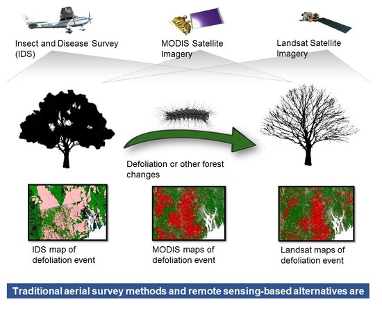
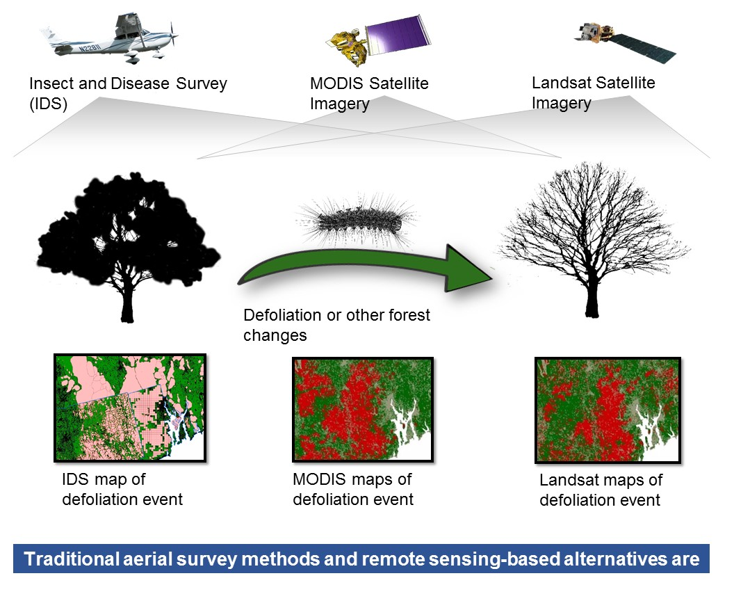
1.1. Aerial Detection Survey
1.2. Remote Sensing Augmentation to IDS
1.3. Change Detection Methods
2. Materials and Methods
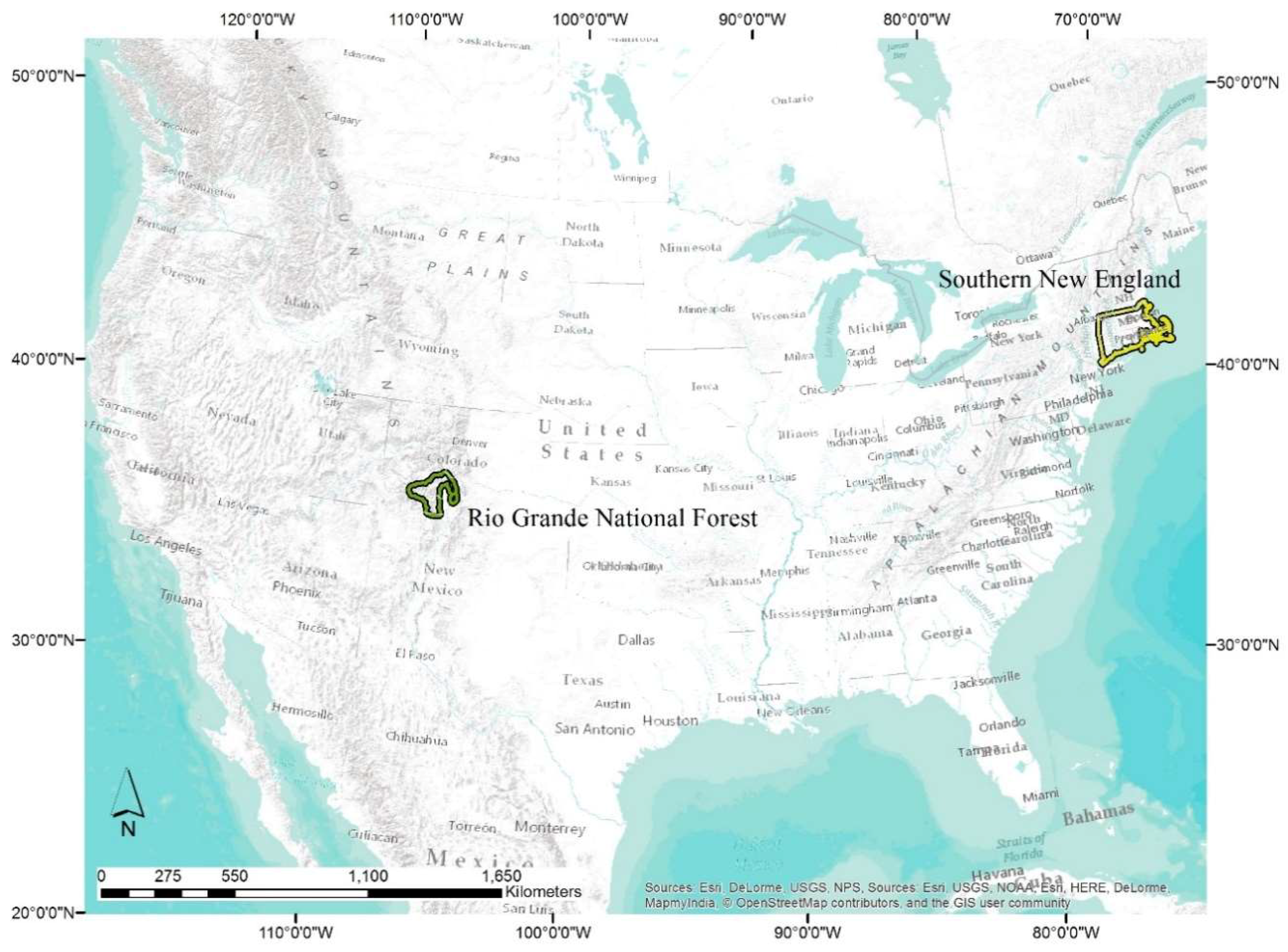
2.1. Study Areas
2.2. IDS-Data
2.3. RTFD-Data
2.4. ORS-Data
2.5. Data Preparation
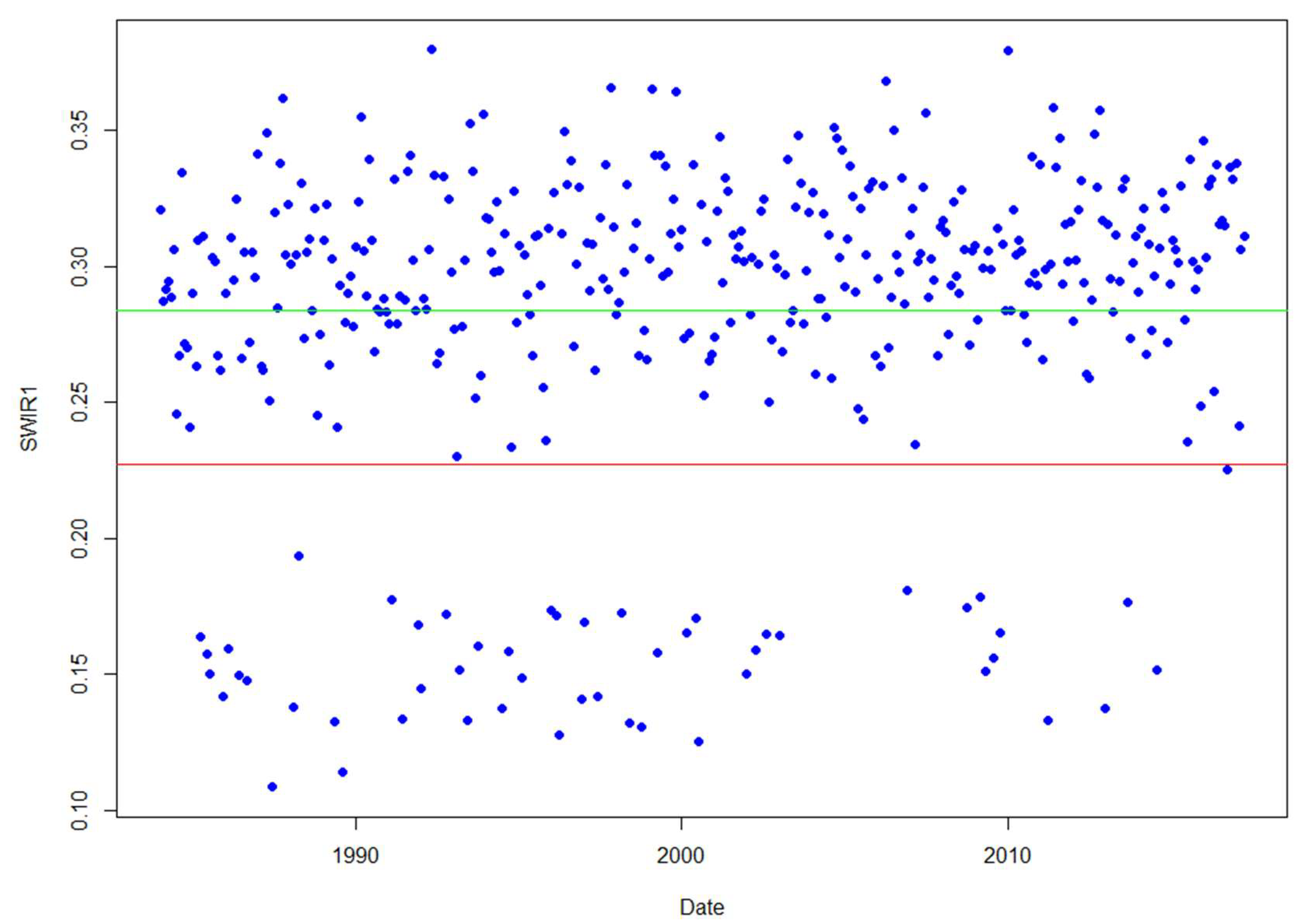
2.6. Change Detection Algorithms
2.7. Accuracy Assessment Methods
3. Results
3.1. Southern New England
3.2. Rio Grande National Forest
4. Discussion
5. Conclusions
Author Contributions
Funding
Acknowledgments
Conflicts of Interest
References
- United States Department of Agriculture. Detection Surveys Overview. Available online: https://www.fs.fed.us/foresthealth/technology/detection_surveys.shtml (accessed on 19 September 2017).
- United States Department of Agriculture. FY10 Mishap Review. Available online: https://www.fs.fed.us/fire/av_safety/assurance/mishaps/FY10_Mishap_Review.pdf (accessed on 21 September 2017).
- Chastain, R.A.; Fisk, H.; Ellenwood, J.R.; Sapio, F.J.; Ruefenacht, B.; Finco, M.V.; Thomas, V. Near-real time delivery of MODIS-based information on forest disturbances. In Time Sensitive Remote Sensing; Lippitt, C.D., Stow, D.A., Coulter, L.L., Eds.; Springer: New York, NY, USA, 2015; pp. 147–164. ISBN 978-1-4939-2601-5. [Google Scholar]
- Coppin, P.R.; Bauer, M.E. Change detection in forest ecosystems with remote sensing digital imagery. Remote Sens. Rev. 1996, 13, 207–234. [Google Scholar] [CrossRef]
- Lu, D.; Mausel, P.; Brondizio, E.; Moran, E. Change detection techniques. Int. J. Remote Sens. 2004, 25, 2365–2407. [Google Scholar] [CrossRef]
- Huang, C.; Goward, S.; Masek, J.; Thomas, N.; Zhu, Z.; Vogelmann, J. An automated approach for reconstructing recent forest disturbance history using dense Landsat time series stacks. Remote Sens. Environ. 2010, 114, 183–198. [Google Scholar] [CrossRef]
- Kennedy, R.; Yang, Z.; Cohen, W. Detecting trends in forest disturbance and recovery using Landsat time series: 1. LandTrendr—Temporal segmentation algorithms. Remote Sens. Environ. 2010, 114, 2897–2910. [Google Scholar] [CrossRef]
- Verbesselt, J.; Hyndman, R.; Newnham, G.; Culvenor, D. Detecting trend and seasonal changes in satellite image time series. Remote Sens. Environ. 2010, 114, 106–115. [Google Scholar] [CrossRef]
- Stueve, K.M.; Housman, I.W.; Zimmerman, P.L.; Nelson, M.D.; Webb, J.B.; Perry, C.H.; Chastain, R.A.; Gormanson, D.D.; Huang, C.; Healey, S.P.; et al. Snow-covered Landsat time series stacks improve automated disturbance mapping accuracy in forested landscapes. Remote Sens. Environ. 2011, 115, 3203–3219. [Google Scholar] [CrossRef]
- Zhu, Z.; Woodcock, C. Continuous change detection and classification of land cover using all available Landsat data. Remote Sens. Environ. 2014, 144, 152–171. [Google Scholar] [CrossRef]
- Verbesselt, J.; Zeileis, A.; Herold, M. Near real-time disturbance detection using satellite image time series. Remote Sens. Environ. 2012, 123, 98–108. [Google Scholar] [CrossRef]
- Brooks, E.B.; Wynne, R.H.; Thomas, V.A.; Blinn, C.E.; Coulston, J.W. On-the-Fly massively multitemporal change detection using statistical quality control charts and Landsat data. IEEE Trans. Geosci. Remote Sens. 2014, 52, 3316–3332. [Google Scholar] [CrossRef]
- Cohen, W.B.; Yang, Z.; Kennedy, R. Detecting trends in forest disturbance and recovery using yearly Landsat time series: 2. TimeSync—Tools for calibration and validation. Remote Sens. Environ. 2010, 114, 2911–2924. [Google Scholar] [CrossRef]
- Griffiths, P.; Kuemmerle, T.; Kennedy, R.E.; Abrudan, I.V.; Knorn, J.; Hostert, P. Using annual time-series of Landsat images to assess the effects of forest restitution in post-socialist Romania. Remote Sens. Environ. 2012, 118, 199–214. [Google Scholar] [CrossRef]
- Cohen, W.B.; Healey, S.P.; Yang, Z.; Stehman, S.V.; Brewer, C.K.; Brooks, E.B.; Gorelick, N.; Huang, C.; Hughes, M.J.; Kennedy, R.E.; et al. How similar are forest disturbance maps derived from different Landsat time series algorithms? Forests 2017, 8, 98. [Google Scholar] [CrossRef]
- United States Forest Service. Available online: https://www.fs.usda.gov/detailfull/riogrande/home/?cid=stelprdb5409285&width=full (accessed on 15 May 2018).
- Ruefenacht, B.; Benton, R.; Johnson, V.; Biswas, T.; Baker, C.; Finco, M.; Megown, K.; Coulston, J.; Winterberger, K.; Riley, M. Forest service contributions to the national land cover database (NLCD): Tree Canopy Cover Production. In Pushing Boundaries: New Directions in Inventory Techniques and Applications: Forest Inventory and Analysis (FIA) Symposium 2015, Portland, OR, USA, 8–10 December 2015; Stanton, S.M., Christensen, G.A., Eds.; U.S. Department of Agriculture, Forest Service, Pacific Northwest Research Station: Portland, OR, USA, 2015; pp. 241–243. [Google Scholar]
- Johnson, E.W.; Wittwer, D. Aerial Detection Surveys in the United States. In Monitoring Science and Technology Symposium: Unifying Knowledge for Sustainability in the Western Hemisphere Proceedings RMRS-P-42CD; Aguirre-Bravo, C., Pellicane, P.J., Burns, D.P., Draggan, S., Eds.; U.S. Department of Agriculture, Forest Service, Rocky Mountain Research Station: Fort Collins, CO, USA, 2006; pp. 809–811. [Google Scholar]
- Department of the Interior U.S. Geological Survey. Product Guide. Landsat 4–7 Surface Reflectance (LEDAPS) Product. Available online: https://landsat.usgs.gov/sites/default/files/documents/ledaps_product_guide.pdf (accessed on 20 June 2018).
- Department of the Interior U.S. Geological Survey. Product Guide. Landsat 8 Surface Reflectance Code (LaSRC) Product. Available online: https://landsat.usgs.gov/sites/default/files/documents/lasrc_product_guide.pdf (accessed on 20 June 2018).
- Gorelick, N.; Hancher, M.; Dixon, M.; Ilyushchenko, S.; Thau, D.; Moore, R. Google Earth Engine: Planetary-scale geospatial analysis for everyone. Remote Sens. Environ. 2017, 202, 18–27. [Google Scholar] [CrossRef]
- Housman, I.; Hancher, M.; Stam, C. A quantitative evaluation of cloud and cloud shadow masking algorithms available in Google Earth Engine. Manuscript in preparation.
- Rouse, J.W.; Haas, R.H., Jr.; Schell, J.A.; Deering, D.W. Monitoring Vegetation Systems in the Great Plains with ERTS; Third ERTS-1 Symposium; NASA: Washington, DC, USA, 1974; pp. 309–317.
- Key, C.H.; Benson, N.C. Landscape Assessment: Ground Measure of Severity, the Composite Burn Index; and Remote Sensing of Severity, the Normalized Burn Ratio; RMRS-GTR-164-CD: LA 1-51; USDA Forest Service, Rocky Mountain Research Station: Ogden, UT, USA, 2006.
- Vogelmann, J.; Xian, G.; Homer, C.; Tolk, B. Monitoring gradual ecosystem change using Landsat time series analyses: Case studies in selected forest and rangeland ecosystems. Remote Sens. Environ. 2012, 12, 92–105. [Google Scholar] [CrossRef]
- Olofsson, P.; Foody, G.M.; Herold, M.; Stehman, S.; Woodcock, C.E.; Wulder, M.A. Good practices for estimating area and assessing accuracy of land change. Remote Sens. Environ. 2014, 148, 42–57. [Google Scholar] [CrossRef]
- Pontius, R.G.; Millones, M. Death to Kappa: Birth of quantity disagreement and allocation disagreement for accuracy assessment. Int. J. Remote Sens. 2011, 32, 4407–4429. [Google Scholar] [CrossRef]
- Healey, S.P.; Cohen, W.B.; Yang, Z.; Brewer, K.; Brooks, E.B.; Gorelick, N.; Hernandez, A.J.; Huang, C.; Hughes, M.J.; Kennedy, R.E.; et al. Mapping forest change using stacked generalization: An ensemble approach. Remote Sens. Environ. 2018, 204, 717–728. [Google Scholar] [CrossRef]
- Pengra, B.; Gallant, A.L.; Zhu, Z.; Dahal, D. Evaluation of the initial thematic output from a continuous change-detection algorithm for use in automated operational land-change mapping by the U.S. Geological Survey. Remote Sens. 2016, 8, 811. [Google Scholar] [CrossRef]
- Brooks, E.B.; Yang, Z.; Thomas, V.A.; Wynne, R.H. Edyn: Dynamic signaling of changes to forests using exponentially weighted moving average charts. Forests 2017, 8, 304. [Google Scholar] [CrossRef]
- COPE-SERCO-RP-17-0186: Sentinel Data Access Annual Report 2017. Available online: https://scihub.copernicus.eu/twiki/pub/SciHubWebPortal/AnnualReport2017/COPE-SERCO-RP-17-0186_-_Sentinel_Data_Access_Annual_Report_2017-Final_v1.4.1.pdf (accessed on 8 June 2018).
- United States Geological Survey. Available online: https://landsat.usgs.gov/using-usgs-spectral-viewer (accessed on 5 August 2017).
- Thomas, V.; (Forest Health Assessment and Applications Sciences Team, Fort Collins, CO, USA). Personal communication, 2017.


| Name | Primary Forest Change Agent | Delineation Method | Area |
|---|---|---|---|
| Rio Grande National Forest | Mountain pine beetle (Dendroctonus ponderosae) and spruce bark beetle (Dendroctonus rufipennis) | Rio Grande National Forest boundary buffered by 10 km | 1,712,261 ha (4,231,089 acres) |
| Southern New England | Gypsy moth (Lymantria dispar dispar) | Union of CT, RI, and MA | 3,680,837 ha (9,095,547 acres) |
| Product Code | Platform | Spatial Resolution | Bands Used |
|---|---|---|---|
| MYD09Q1 | Aqua | 250 m | red, NIR |
| MOD09Q1 | Terra | 250 m | red, NIR |
| MYD09A1 | Aqua | 500 m | blue, green, SWIR1, SWIR2 |
| MOD09A1 | Terra | 500 m | blue, green, SWIR1, SWIR2 |
| ORS Method | Platform | Index | Overall Accuracy | 5% CI | 95% CI | Tree No Change Commission Error Rate | Tree No Change Omission Error Rate | Tree Change Commission Error Rate | Tree Change Omission Error Rate | Tree Change Reference Prevalence | Tree Change Predicted Prevalence |
|---|---|---|---|---|---|---|---|---|---|---|---|
| Harmonic | Landsat | NBR | 89.18% | 86.78% | 91.36% | 2.29% | 9.76% | 56.06% | 21.62% | 8.89% | 15.87% |
| Harmonic | Landsat | NDVI | 89.66% | 86.78% | 92.07% | 4.59% | 6.86% | 56.52% | 45.95% | 8.89% | 11.06% |
| Harmonic | MODIS | NBR | 88.70% | 86.06% | 91.35% | 4.14% | 8.44% | 59.26% | 40.54% | 8.89% | 12.98% |
| Harmonic | MODIS | NDVI | 91.59% | 89.42% | 93.75% | 7.43% | 1.32% | 41.67% | 81.08% | 8.89% | 2.88% |
| Basic | Landsat | NBR | 86.06% | 83.17% | 88.70% | 0.62% | 14.78% | 61.54% | 5.41% | 8.89% | 21.88% |
| Basic | Landsat | NDVI | 91.83% | 89.42% | 94.23% | 4.00% | 5.01% | 46.34% | 40.54% | 8.89% | 9.86% |
| Basic | MODIS | NBR | 92.07% | 90.14% | 94.23% | 3.99% | 4.75% | 45.00% | 40.54% | 8.89% | 9.62% |
| Basic | MODIS | NDVI | 91.35% | 89.17% | 93.51% | 7.23% | 1.85% | 46.67% | 78.38% | 8.89% | 3.61% |
| Trend | Landsat | NBR | 91.35% | 89.18% | 93.51% | 1.96% | 7.65% | 49.15% | 18.92% | 8.89% | 14.18% |
| Trend | Landsat | NDVI | 92.55% | 90.63% | 94.47% | 3.97% | 4.22% | 42.11% | 40.54% | 8.89% | 9.13% |
| Trend | MODIS | NBR | 91.35% | 88.94% | 93.51% | 2.75% | 6.86% | 49.06% | 27.03% | 8.89% | 12.74% |
| Trend | MODIS | NDVI | 91.83% | 89.66% | 93.75% | 5.66% | 3.17% | 44.44% | 59.46% | 8.89% | 6.49% |
| RTFD | MODIS | NDMI | 84.86% | 82.21% | 87.75% | 5.11% | 11.87% | 70.31% | 48.65% | 8.89% | 15.38% |
| IDS | -- | -- | 89.18% | 87.01% | 91.83% | 6.05% | 5.80% | 61.11% | 62.16% | 8.89% | 8.65% |
| ORS Method | Platform | Index | Overall Accuracy | 5% CI | 95% CI | Tree No Change Commission Error Rate | Tree No Change Omission Error Rate | Tree Change Commission Error Rate | Tree Change Omission Error Rate | Tree Change Reference Prevalence | Tree Change Predicted Prevalence |
|---|---|---|---|---|---|---|---|---|---|---|---|
| Harmonic | Landsat | NBR | 78.61% | 75.24% | 81.73% | 5.96% | 21.18% | 54.96% | 22.37% | 18.27% | 31.49% |
| Harmonic | Landsat | NDVI | 73.80% | 69.71% | 77.40% | 9.19% | 24.41% | 62.41% | 34.21% | 18.27% | 31.97% |
| Harmonic | MODIS | NBR | 71.63% | 68.03% | 75.00% | 8.58% | 27.94% | 64.19% | 30.26% | 18.27% | 35.58% |
| Harmonic | MODIS | NDVI | 80.77% | 77.64% | 83.89% | 16.67% | 4.41% | 57.69% | 85.53% | 18.27% | 6.25% |
| Basic | Landsat | NBR | 80.29% | 77.40% | 83.17% | 3.93% | 20.88% | 52.21% | 14.47% | 18.27% | 32.69% |
| Basic | Landsat | NDVI | 77.88% | 74.76% | 81.01% | 10.26% | 17.65% | 57.69% | 42.11% | 18.27% | 25.00% |
| Basic | MODIS | NBR | 80.05% | 76.91% | 83.65% | 11.18% | 13.53% | 54.12% | 48.68% | 18.27% | 20.43% |
| Basic | MODIS | NDVI | 81.49% | 78.37% | 84.38% | 14.56% | 6.76% | 51.11% | 71.05% | 18.27% | 10.82% |
| Trend | Landsat | NBR | 86.30% | 83.65% | 88.94% | 4.21% | 12.94% | 41.12% | 17.11% | 18.27% | 25.72% |
| Trend | Landsat | NDVI | 81.49% | 78.37% | 84.39% | 7.44% | 15.88% | 50.47% | 30.26% | 18.27% | 25.72% |
| Trend | MODIS | NBR | 87.02% | 84.13% | 89.66% | 7.94% | 7.94% | 35.53% | 35.53% | 18.27% | 18.27% |
| Trend | MODIS | NDVI | 85.82% | 82.93% | 88.46% | 12.73% | 3.24% | 28.21% | 63.16% | 18.27% | 9.38% |
| RTFD | MODIS | NDMI | 84.38% | 81.25% | 87.26% | 11.27% | 7.35% | 40.98% | 52.63% | 18.27% | 14.66% |
| IDS | -- | -- | 79.81% | 76.68% | 82.93% | 8.97% | 16.47% | 53.85% | 36.84% | 18.27% | 25.00% |
| ORS Method | Platform | Index | Overall Accuracy | 5% CI | 95% CI | Tree No Change Commission Error Rate | Tree No Change Omission Error Rate | Tree Change Commission Error Rate | Tree Change Omission Error Rate | Tree Change Reference Prevalence | Tree Change Predicted Prevalence |
|---|---|---|---|---|---|---|---|---|---|---|---|
| Harmonic | Landsat | NBR | 63.48% | 58.70% | 69.13% | 17.29% | 35.67% | 62.89% | 38.98% | 25.65% | 42.17% |
| Harmonic | Landsat | NDVI | 69.57% | 64.78% | 73.91% | 25.37% | 10.53% | 72.00% | 88.14% | 25.65% | 10.87% |
| Harmonic | MODIS | NBR | 75.65% | 71.30% | 80.43% | 14.29% | 19.30% | 47.83% | 38.98% | 25.65% | 30.00% |
| Harmonic | MODIS | NDVI | 75.22% | 70.87% | 79.57% | 22.86% | 5.26% | 45.00% | 81.36% | 25.65% | 8.70% |
| Basic | Landsat | NBR | 71.74% | 66.96% | 76.09% | 10.45% | 29.82% | 53.13% | 23.73% | 25.65% | 41.74% |
| Basic | Landsat | NDVI | 74.35% | 69.57% | 79.13% | 24.31% | 3.51% | 50.00% | 89.83% | 25.65% | 5.22% |
| Basic | MODIS | NBR | 76.09% | 71.30% | 81.30% | 16.28% | 15.79% | 46.55% | 47.46% | 25.65% | 25.22% |
| Basic | MODIS | NDVI | 77.83% | 73.48% | 82.61% | 21.43% | 3.51% | 30.00% | 76.27% | 25.65% | 8.70% |
| Trend | Landsat | NBR | 75.65% | 71.30% | 80.00% | 15.98% | 16.96% | 47.54% | 45.76% | 25.65% | 26.52% |
| Trend | Landsat | NDVI | 79.13% | 74.78% | 83.48% | 20.29% | 3.51% | 26.09% | 71.19% | 25.65% | 10.00% |
| Trend | MODIS | NBR | 76.52% | 71.74% | 80.87% | 18.03% | 12.28% | 44.68% | 55.93% | 25.65% | 20.43% |
| Trend | MODIS | NDVI | 78.26% | 73.91% | 82.61% | 20.77% | 4.09% | 30.43% | 72.88% | 25.65% | 10.00% |
| RTFD | MODIS | NDMI | 71.30% | 66.52% | 75.67% | 23.35% | 11.70% | 60.61% | 77.97% | 25.65% | 14.35% |
| IDS | -- | -- | 75.65% | 71.30% | 80.43% | 19.58% | 11.11% | 46.34% | 62.71% | 25.65% | 17.83% |
| ORS Method | Platform | Index | Overall Accuracy | 5% CI | 95% CI | Tree No Change Commission Error Rate | Tree No Change Omission Error Rate | Tree Change Commission Error Rate | Tree Change Omission Error Rate | Tree Change Reference Prevalence | Tree Change Predicted Prevalence |
|---|---|---|---|---|---|---|---|---|---|---|---|
| Harmonic | Landsat | NBR | 66.09% | 60.87% | 71.30% | 16.67% | 35.19% | 54.81% | 30.88% | 29.57% | 45.22% |
| Harmonic | Landsat | NDVI | 68.70% | 63.48% | 73.91% | 28.77% | 6.79% | 61.11% | 89.71% | 29.57% | 7.83% |
| Harmonic | MODIS | NBR | 68.70% | 63.48% | 73.91% | 19.59% | 26.54% | 52.44% | 42.65% | 29.57% | 35.65% |
| Harmonic | MODIS | NDVI | 67.83% | 62.61% | 73.04% | 28.64% | 9.26% | 62.50% | 86.76% | 29.57% | 10.43% |
| Basic | Landsat | NBR | 67.83% | 63.46% | 72.61% | 10.00% | 38.89% | 52.50% | 16.18% | 29.57% | 52.17% |
| Basic | Landsat | NDVI | 71.30% | 66.09% | 76.09% | 28.38% | 1.85% | 37.50% | 92.65% | 29.57% | 3.48% |
| Basic | MODIS | NBR | 76.09% | 71.72% | 80.00% | 19.08% | 13.58% | 38.60% | 48.53% | 29.57% | 24.78% |
| Basic | MODIS | NDVI | 70.87% | 66.07% | 75.65% | 26.83% | 7.41% | 48.00% | 80.88% | 29.57% | 10.87% |
| Trend | Landsat | NBR | 75.22% | 70.87% | 79.57% | 15.23% | 20.99% | 43.04% | 33.82% | 29.57% | 34.35% |
| Trend | Landsat | NDVI | 75.65% | 70.87% | 80.43% | 25.23% | 1.23% | 12.50% | 79.41% | 29.57% | 6.96% |
| Trend | MODIS | NBR | 75.22% | 70.41% | 80.00% | 20.34% | 12.96% | 39.62% | 52.94% | 29.57% | 23.04% |
| Trend | MODIS | NDVI | 76.09% | 71.30% | 80.87% | 23.65% | 4.32% | 25.93% | 70.59% | 29.57% | 11.74% |
| RTFD | MODIS | NDMI | 71.74% | 66.96% | 76.54% | 27.01% | 4.94% | 42.11% | 83.82% | 29.57% | 8.26% |
| IDS | -- | -- | 67.83% | 63.04% | 72.61% | 26.09% | 16.05% | 56.52% | 70.59% | 29.57% | 20.00% |
© 2018 by the authors. Licensee MDPI, Basel, Switzerland. This article is an open access article distributed under the terms and conditions of the Creative Commons Attribution (CC BY) license (http://creativecommons.org/licenses/by/4.0/).
Share and Cite
Housman, I.W.; Chastain, R.A.; Finco, M.V. An Evaluation of Forest Health Insect and Disease Survey Data and Satellite-Based Remote Sensing Forest Change Detection Methods: Case Studies in the United States. Remote Sens. 2018, 10, 1184. https://doi.org/10.3390/rs10081184
Housman IW, Chastain RA, Finco MV. An Evaluation of Forest Health Insect and Disease Survey Data and Satellite-Based Remote Sensing Forest Change Detection Methods: Case Studies in the United States. Remote Sensing. 2018; 10(8):1184. https://doi.org/10.3390/rs10081184
Chicago/Turabian StyleHousman, Ian W., Robert A. Chastain, and Mark V. Finco. 2018. "An Evaluation of Forest Health Insect and Disease Survey Data and Satellite-Based Remote Sensing Forest Change Detection Methods: Case Studies in the United States" Remote Sensing 10, no. 8: 1184. https://doi.org/10.3390/rs10081184
APA StyleHousman, I. W., Chastain, R. A., & Finco, M. V. (2018). An Evaluation of Forest Health Insect and Disease Survey Data and Satellite-Based Remote Sensing Forest Change Detection Methods: Case Studies in the United States. Remote Sensing, 10(8), 1184. https://doi.org/10.3390/rs10081184