Using 250-M Surface Reflectance MODIS Aqua/Terra Product to Estimate Turbidity in a Macro-Tidal Harbour: Darwin Harbour, Australia

Abstract

Turbidity is an indicator of the quality of water and usually exhibits variability associated with changing hydrodynamic conditions, which can be reflected in the sediment dynamics in coastal regions. Darwin Harbour is a typical macro-tidal, well mixed, and complex environment influenced by industries, human activities, and natural factors—including winds, currents, river discharges, waves, and tides. As a case study, hydrodynamics and sediment dynamics in Darwin Harbour are investigated using moderate resolution imaging spectroradiometer (MODIS) measurements. This study focuses on understanding the variability of turbidity, mechanisms that control the variations of turbidity and analyzing field data to determine the main factors that influence the sediment dynamics in Darwin Harbour. The results of this study illustrate the seasonal turbidity variation is mainly influenced by the wind waves. The dredging campaigns in 2013 and 2014 wet seasons contributed to the rise of turbidity in Darwin Harbour. The action of tidal currents appears to be the dominant factor controlling the turbidity pattern in a spring–neap cycle and the turbidity intra-tidal variation. In addition, the turbidity maximum zone (TMZ) near Charles Point is formed by the tidal current convergence based on the results of current modelling.

1. Introduction

A coastal zone is an area between land and ocean where a large variety of materials and energy interact. The population and number of large-scale industries in coastal areas have increased dramatically in recent decades and this contributes to both water pollution and damage to sensitive coastal ecosystems. Thus, monitoring coastal water quality as part of the management of harbours and marine industries is essential to control water pollution and protect these coastal habitats. Turbidity is an index of light attenuation and water quality and is important for understanding coastal erosion, as well as agricultural and urban nutrient discharges [1]. Therefore, monitoring dynamic variations of surface turbidity in coastal areas is important for understanding coastal sedimentary processes and dynamics [2,3,4,5].

The measurement of turbidity in coastal areas using conventional in situ methods at fixed stations provides long time series of high-quality measurements of turbidity. However, because of its heterogeneous structure, continuous measurement of turbidity at individual locations fails to properly capture the spatial patterns in turbidity due to natural forcings on diurnal, monthly, and seasonal scales. Application of satellite-based ocean sensors to monitor water quality has considerable advantages compared with in situ measurements and can be used to assess water quality in large areas but satellite data also has the limitations to capture the vertical sediment concentrations. Several well-known ocean color sensors, such as the sea-viewing Wide Field-of-view Sensor (SeaWiFs) [6,7,8,9], MODIS [1,3,10,11,12,13], Landsat series [14,15,16,17,18], the Geostationary Ocean Color Imager (GOCI) [4,19,20], and the Medium Resolution Imaging Spectrometer (MERIS) [21,22] have been widely used for the retrieval of instantaneous horizontal distributions of turbidity in order to observe seasonal movements of turbidity in coastal areas. This study uses MODIS instrument, which is on the Aqua and Terra satellites, as a tool to derive the turbidity in Darwin Harbour and coastal areas in and around Darwin Harbour.

MODIS is a scientific sensor launched by NASA aboard the Terra (1999) and aboard the Aqua (2002) satellites resulting a return rate over a given location of approximately one day. The equator crossing time for Terra is 10:30 a.m. (descending node) and 1:30 p.m. for Aqua (ascending node), and two images per day can be obtained by combining the MODIS imagery from both Aqua and Terra. MODIS has 36 spectral bands from 0.4 μm to 14.4 μm and various spatial resolutions at 250-m, 500-m, and 1-km resolution. The multi-spectral resolution improves observational capability of the earth system including the surface. The high spatial and temporal resolution can provide an optimal method to detect a variety of environmental disasters and changes in local areas [11]. Thus, detecting water turbidity using MODIS is an effective way to understand and monitor sediment transport, changes of topography, and water pollution, which can then be used to protect and manage the vulnerable coastal environment.

The MODIS Aqua and Terra surface reflectance product (MOD09GQ for Terra, MYD09GQ for Aqua) has already been atmospherically corrected and is currently available. These data have been proven to be used to estimate turbidity and suspended sediment concentration (SSC) in number of previous studies [1,12,23,24].

In this study, the MODIS products band 1 (645 nm) reflectance data are used to retrieve turbidity in Darwin Harbour in order to better understand its spatial and temporal distribution. Darwin Harbour and adjacent coastal waters are typical macro-tidal and well-mixed regions, connecting the Elizabeth and Blackmore River with the outer Darwin Harbour (Figure 1). Coastal industries, including import and export trade, tourism, and transportation has developed rapidly in Darwin Harbour, resulting in increased investment and growth in the population. According to Andutta et al. [25], the population will rise up to ~335,000 people in the next 40 years from ~146,000 in 2016. Such a rapid rise is likely to put a high amount of stress on the ecological environment. The dredging activity was frequent in Darwin Harbour causing large amount of fine sediment poured into this area causing huge impact on environment of sea. Other natural factors including wind, tides, and river discharge complicate the coastal hydrodynamics environment in this region making it important to understand the driving mechanisms behind the seasonal to intra-tidal variations in turbidity within the harbour area.

The objectives of this study are to describe the seasonal, intra-tidal turbidity variations, and influence of tides on the turbidity distribution in and around Darwin Harbour using the MODIS reflectance data combined with in situ observations and numerical modelling results. Specific aims are to: (1) understand the turbidity seasonal variation in Darwin Harbour; (2) understand the effect of the spring–neap tide on the magnitude and distribution of turbidity in Darwin Harbour; (3) analyze the intra-tidal turbidity at different tidal phases (ebb tide, low water level, flood tide, and high water level); and (4) to investigate the mechanisms that control the formation of the turbidity maximum zone in Darwin Harbour use modelling studies. The rest of the paper is structured in the following way. Section 2 describes the study area, data, and methods used to retrieve turbidity and analyze its characteristics. Results of the analysis of the turbidity and the influence of various natural forcings on its spatial structure are discussed in Section 3. Conclusions are provided in Section 4.

2. Data and Methods

2.1. Study Area

Darwin Harbour (12°28′S, 130°51′E) is a semi diurnal macro-tidal estuary near Darwin on the north coast of the Northern Territory of Australia. It has 3 arms: the West Arm (WA), the Middle Arm (MA) and the East Arm (EA) (Figure 1). The tidal range in Darwin Harbour varies during the spring- neap tide cycle, with a mean 5.5 m spring and 1.9 m neap range. The maximum tidal range can be as high as 7.8 m [25,26,27,28]. Soft surfaces consisting of muds and fine sand are estimated to cover approximately 80% of the study domain [27,28]. According to McKinnon et al. [29], the concentration of chlorophyll in Darwin Harbour is low, with 0.77 μg/L in the wet season and 0.89 μg/L in the dry season. Darwin Harbour is a flooded river valley system with two main rivers, the Blackmore River and Elizabeth River. According to Padovan [30], the seasonal river discharge fluctuates seasonally, with 605 and 389 ML/day for these two rivers in January, decreasing to zero by July when there is no freshwater input into Darwin Harbour until the following wet season. The water depth ranges from 0 to 20 m, with a maximum of about 40 m in coastal areas [25].

The Darwin Harbour area is dominated by a tropical climate with an average annual rainfall of 1,729 mm. The wet season (November to April) has mean rainfall of 269 mm/month and is dominated by cyclone activity. During the dry season (May to October), the rainfall decreases substantially to 19.3 mm/month (Australian Bureau of Meteorology, 2017).

2.2. Observational Data

Observational data, including wind, wave, tide, and turbidity from November 2012 to October 2017 for an IMOS station located at 12.34°S, 130.69°E in the outer harbour were downloaded from the Australian Institute of Marine Science (AIMS) (https://www.aims.gov.au/docs/data/data.html). The instrument used to measure turbidity is the Wetlabs Water Quality Monitor. The surface turbidity was used to calibrate the MODIS reflectance data. Monthly averaged river discharge was obtained from the Water Data Portal (https://nt.gov.au/environment/water/water-data-portal).

2.3. MODIS Data

Aqua and Terra are two polar-orbiting satellites launched by the U.S. National Aeronautics and Space Agency (NASA) in 1999 and 2002, respectively, which carry MODIS sensors with 36 spectral channels. Important advantages of MODIS are the length of the time series of measurements and the high 250-m spatial resolution. The surface reflectance data (MYD09GQ and MOD09GQ) were downloaded from 1 November 2012 to 31 October 2017, from the Land Processes Distributed Active Archive Center (LP DAAC) of the US Geological Survey (USGS) and NASA. These surface reflectance data are geolocated and atmospherically corrected. Doxaran et al. [2] described the detailed atmospheric correction process for this product. The data are not corrected for skylight reflection at the atmosphere–ocean interface and are not accurate enough for open ocean applications. However, the data are appropriate for application in turbid coastal waters [2]. The MODIS images were processed by the MODIS Reprojection Tool (MRT) and ENVI version 5.1. For images covered by clouds, the methodology based on band 2 was applied to remove cloud contamination [2,3,12]. Many studies have tested this product and the reflectance was found to have significant correlation with in situ turbidity measurements and SSC in coastal areas [1,12,23,24].

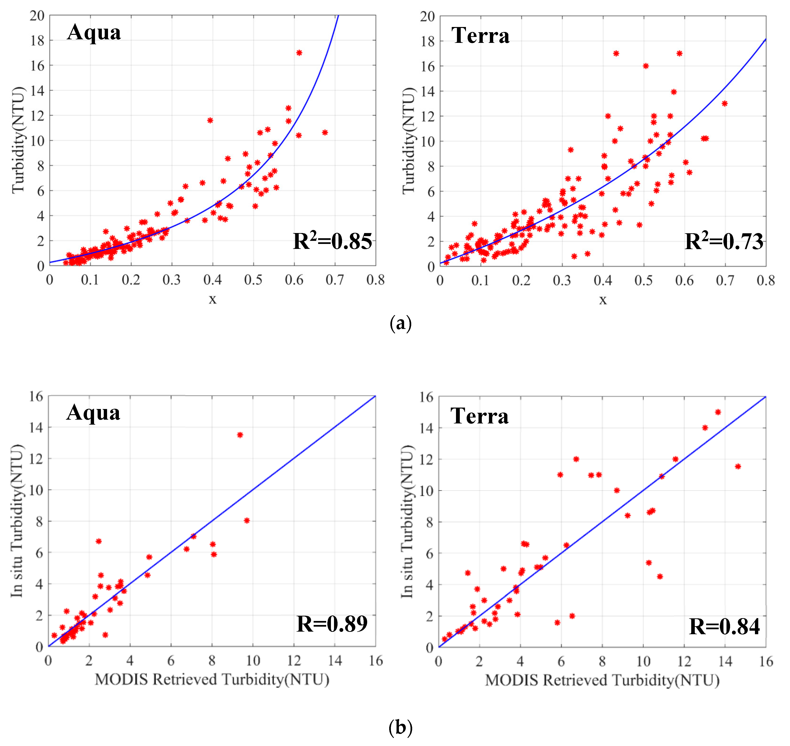
2.4. Turbidity Retrieval Algorithm

Many studies have developed algorithms to retrieve SSC and turbidity, using the correlation between in situ observations and the reflectance measurements obtained by MODIS and other ocean color sensors [1,11,23,31]. The algorithm used for this study is based on the semi-analytic sediment model (SASM), which was applied to MODIS-Aqua observations by Dorji et al. [32]. They developed the model to retrieve SSC in northern Western Australia based on radiative transfer algorithms and it performs better than other linear, polynomial, and exponential models [32,33,34]. The model is given by

$$\mathrm{Turbidity}=\frac{\mathrm{a}\times \left(\frac{\mathrm{x}}{1-\mathrm{x}}\right)}{1-\mathrm{b}\times \left(\frac{\mathrm{x}}{1-\mathrm{x}}\right)}+\mathrm{c}$$

(1)

where $\mathrm{x}=\frac{-{\mathrm{g}}_1+\sqrt{{\left({\mathrm{g}}_1\right)}^2+4\times {\mathrm{g}}_2{\times \mathrm{r}}_{\mathrm{s}}}}{2\times {\mathrm{g}}_2}$, ${\mathrm{g}}_1=0.084$, ${\mathrm{g}}_2$ = 0.17, ${\mathrm{r}}_{\mathrm{s}}=\frac{{\mathrm{R}}_{\mathrm{rs}}}{0.52+1.7\times {\mathrm{R}}_{\mathrm{rs}}}$, ${\mathrm{R}}_{\mathrm{rs}}$ is the atmospherically corrected MODIS band 1 reflectance, and a, b, and c are derived parameters using regression analysis between the in situ turbidity measurements and x.

In order to calibrate and test the model, 184 reflectance datasets for Aqua (135 for calibrating, 49 for validation), and 198 datasets for Terra (150 for calibrating, 48 for validation), were randomly selected from the period November 2012–October 2017. The resulting calibrated models by Equations (2) and (3) for Aqua and Terra are shown in Figure 2a. Figure 2b and

Table 1. Validation results for the turbidity retrieval algorithm.

	RMSE(NTU)	MAPE	r
Aqua	1.18	33%	0.89
Terra	2.25	34%	0.84

show the comparison between the MODIS retrieved turbidity and observations from the IMOS station with good correlation scores in both cases.

$$\mathrm{Turbidity}=\frac{6.357\times \left(\frac{\mathrm{x}}{1-\mathrm{x}}\right)}{1-0.09\times \left(\frac{\mathrm{x}}{1-\mathrm{x}}\right)}+0.2552$$

(2)

$$\mathrm{Turbidity}=\frac{11.59\times \left(\frac{\mathrm{x}}{1-\mathrm{x}}\right)}{1+0.3694\times \left(\frac{\mathrm{x}}{1-\mathrm{x}}\right)}+0.2451$$

(3)

where the Equations (2) and (3) are used to retrieve turbidity for Aqua and Terra, respectively.

Root mean square error (RSME) and mean absolute percentage error (MAPE) are calculated using

$$\mathrm{RMSE}=\sqrt{\frac{{{\displaystyle \sum }}_{\mathrm{i}=1}^{\mathrm{n}}{\left({\mathrm{X}}_{\mathrm{obs},\mathrm{i}}-{\mathrm{X}}_{\mathrm{model},\mathrm{i}}\right)}^2}{\mathrm{n}}}$$

(4)

$$\mathrm{MAPE}=\frac{{\mathrm{\Sigma }}_{\mathrm{i}=1}^{\mathrm{n}}\frac{\left|{\mathrm{X}}_{\mathrm{obs},\mathrm{i}}-{\mathrm{X}}_{\mathrm{model},\mathrm{i}}\right|}{{\mathrm{X}}_{\mathrm{obs},\mathrm{i}}}}{\mathrm{n}}\times 100\%$$

(5)

3. Results and Discussion

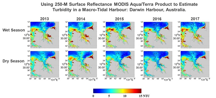
3.1. Seasonal Variation of Turbidity in Darwin Harbour

Turbidity in the Darwin Harbour is influenced by various factors, including wind, river discharge, and tide. To study seasonal variations of turbidity in Darwin Harbour, MODIS passes at the same tidal phase (low water level in spring tides) during the period from November 2012 to October 2017, were chosen and grouped into wet and dry seasons to calculate the time-averaged turbidity distribution. During the wet season, the cloud coverage in the study domain is greater than that in the dry season, and as a result there are less clear or partly cloudy MODIS passes available during the wet season compared to the dry season (

Table 2. The number of clear and partly cloudy day MODIS passes used to retrieve the mean seasonal turbidity in Darwin Harbour.

	2013	2014	2015	2016	2017
Wet season	13	14	11	19	9
Dry season	19	32	25	23	26

).

Transect 1 and the two stations, A (12.37°S, 130.64°E) and B (12.51°S, 130.84°E), were chosen to show the seasonal turbidity variations in the inner and outer harbour (Figure 1). The spatial distribution of the seasonal mean turbidity in Darwin Harbour from November 2012 to October 2017 is shown in Figure 3.

During 2013 to 2017, the turbidity maximum zone (TMZ), which is defined as values greater than 8 NTU was located in the estuary of the Elizabeth and Blackmore Rivers, the area near Charles Point and parallel with the coastline. There is clearly seasonal spatial variation of the turbidity during the chosen period, especially around the west coast near Charles Point and the inner harbour. During the wet season, the turbidity of the inner harbour was at least 8 NTU, which is much higher than that in dry seasons. At the mouth of the Elizabeth and Blackmore Rivers, the turbidity was always high during the wet season. In particular, in 2013 and 2014 the turbidity in the estuary of the Elizabeth River reached 15 NTU. During dry seasons, the turbidity in the inner harbour was lower (6 NTU) and the TMZ was smaller compared with wet seasons. In general, the TMZ was located in a limited region, near coastal areas and the mouth of the rivers. In the outer harbour, seasonal variation of turbidity near Charles Point was high (shown in Figure 4a), increasing to 16 NTU and extending into the deep ocean in wet seasons and decreasing to less than 11 NTU in dry seasons (Figure 4). The TMZ was always located near Charles Point and the area near Nightcliff and East Point (Figure 3). The mechanisms controlling the TMZ will be discussed in Section 3.4.

Figure 4a,b show seasonal variation of the averaged turbidity at station A and B: The stations had similar turbidity patterns, with the wet season turbidity nearly twice that in the dry season especially for the inner harbour.

Factors Controlling the Seasonal Variability of Turbidity

Many factors—such as tides, winds, waves and river discharge—can influence the seasonal variation of turbidity [4]. For coastal areas, the river discharge is regarded as an important factor for seasonal turbidity. High river discharge can form a freshwater front and seaward residual currents, which affects the water circulation, turbulent mixing in the water column and helps to form a turbidity maximum zone [35]. The materials transported by the river flow can also affect the distribution of turbidity.

The cross section from P1 to P2, which is about 36 km long (Figure 1) was chosen to display patterns of turbidity distribution and evaluate the influence of river discharge on the turbidity in the wet and dry season. The seasonal turbidity variability of Darwin Harbour is shown in Figure 4, with a larger turbidity in the inner harbour during the wet season.

During the dry season, the turbidity decreased slightly from about 6 NTU in the inner harbour to about 4 NTU in the outer harbour. In the wet season, the turbidity in the inner harbour was between 7 and 9 NTU while it was similar to the dry season in the outer harbour. The seasonal turbidity pattern along transect 1 was similar for all years with higher turbidity in the wet season compared with the dry season for the inner harbour (Figure 5). In general, the turbidity slowly decreased from the mouth of the estuary to the outer harbour.

According to gauges in the Blackmore River, Berry Creek, and Elizabeth River (Figure 6), the river runoff in the 2017 wet season was significantly higher than other years. Nevertheless, the turbidity along transect 1 in the wet season in 2017 was not much higher than other years. The largest measured river discharge during an exceptional flood, was 1000 m³ s⁻¹, which is about 1% peak tidal discharge at the mouth [36]. This suggests that the influence of river discharge on turbidity in Darwin Harbour was negligible.

It is noteworthy that the wet season turbidity in the East Arm in 2013 and 2014 was much higher than other years (Figure 3a,b), most likely because of dredging activity during the East Arm dredging campaign. During this campaign, there was dredging occurring from November 2012 to April 2013 (Season One) and November 2013 to June 2014 (Season Two). The East Arm has mainly erodible mud seabed [36,37], and large amounts of fine sediment were resuspended in the East Arm and there was a muddy plume arising from a continuous mud discharge from the dredging activity. At the same phase of dredging, the disposal materials would be transported to an offshore dumping area (red box in Figure 3), which contributed to the rise of turbidity near the offshore disposal area during the corresponding period in 2013 and 2014 (Ichthys Nearshore Environmental Monitoring Program, 2015).

Because of the large tidal range in Darwin Harbour, there is no clear river plume in the study domain and the suspended matter is well mixed [36,37]. According to IMOS field wind data (shown in Figure 7), there is a prevailing westerly wind during the wet season, which becomes weaker easterly in the dry season.

Waves generated by the wind acting on the fetch play an important role in re-suspending sediment in estuaries. Strong waves can increase the bed shear stress which can enhance the sediment re-suspension in shallow waters. Waves less than 20 cm high can already resuspend sediment in coastal areas [38]. Apart from waves, residual currents, driven by wind, density, runoff, and bathymetry can also influence the distribution of turbidity. However, in Darwin Harbour, the effects of residual currents are negligible compared with tidal currents [25,37]. Therefore, the effect of waves driven by strong winds will be mainly discussed here.

The significant wave height has a strong relationship (R = 0.74) with wind velocity at the IMOS station (Figure 8). High turbidity there generally corresponded to high significant wave height and strong wind. According to the IMOS field data (

Table 3. Seasonal mean significant wave height and mean wind speed at the IMOS station.

		2013	2014	2015	2016	2017
Significant wave height (m)	Wet season	0.45	0.52	0.51	0.40	0.54
	Dry season	0.17	0.27	0.25	0.26	0.27
Wind speed (m/s)	Wet season	4.11	4.70	4.76	4.20	4.42
	Dry season	4.00	3.69	3.70	3.92	3.77

), from 2013 to 2017, the mean wind velocity and significant wave height in the wet season were much higher than that in the dry season. Higher winds in the wet season can systematically influence the turbidity by causing larger waves and re-suspending larger amounts of sediment on the seabed. In contrast, weaker winds and lower wave heights in the dry season leaded to low turbidity in the study domain. The wave effect on turbidity has also been found in coastal regions around the world, including the Yalu estuary [4], the estuary of the Yangtze River [39], and the English Channel [40]. Through the analysis of variation (ANOVA) [41] for the five years data of the wet and dry seasons, p-value < 0.01 at Station B and =0.04 at IMOS Station, respectively, indicating the turbidity seasonal variation in the inner harbour is more significant, compared with the deep waters in the outer harbour. This is because suspended sediment driven by waves is an important resuspension mechanism in shallow estuaries and coastal areas [42] and the sediment in shallow water can be easily carried to the water surface by strong waves. Hence, due to the smaller water depth, the seasonal variation in turbidity in the inner harbour and coastal areas was more notable than that in the outer harbour.

In general, these outcomes suggest that wind driven waves was a major factor controlling the seasonal variation of turbidity in Darwin Harbour and offshore areas.

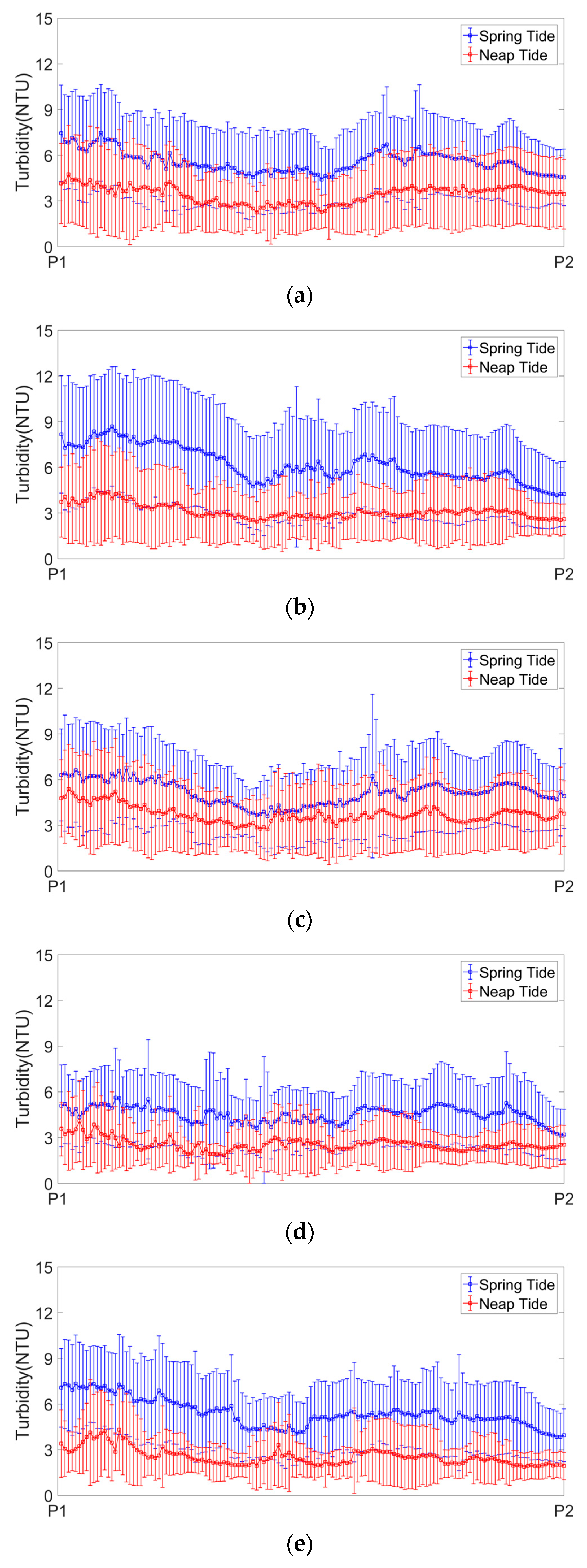
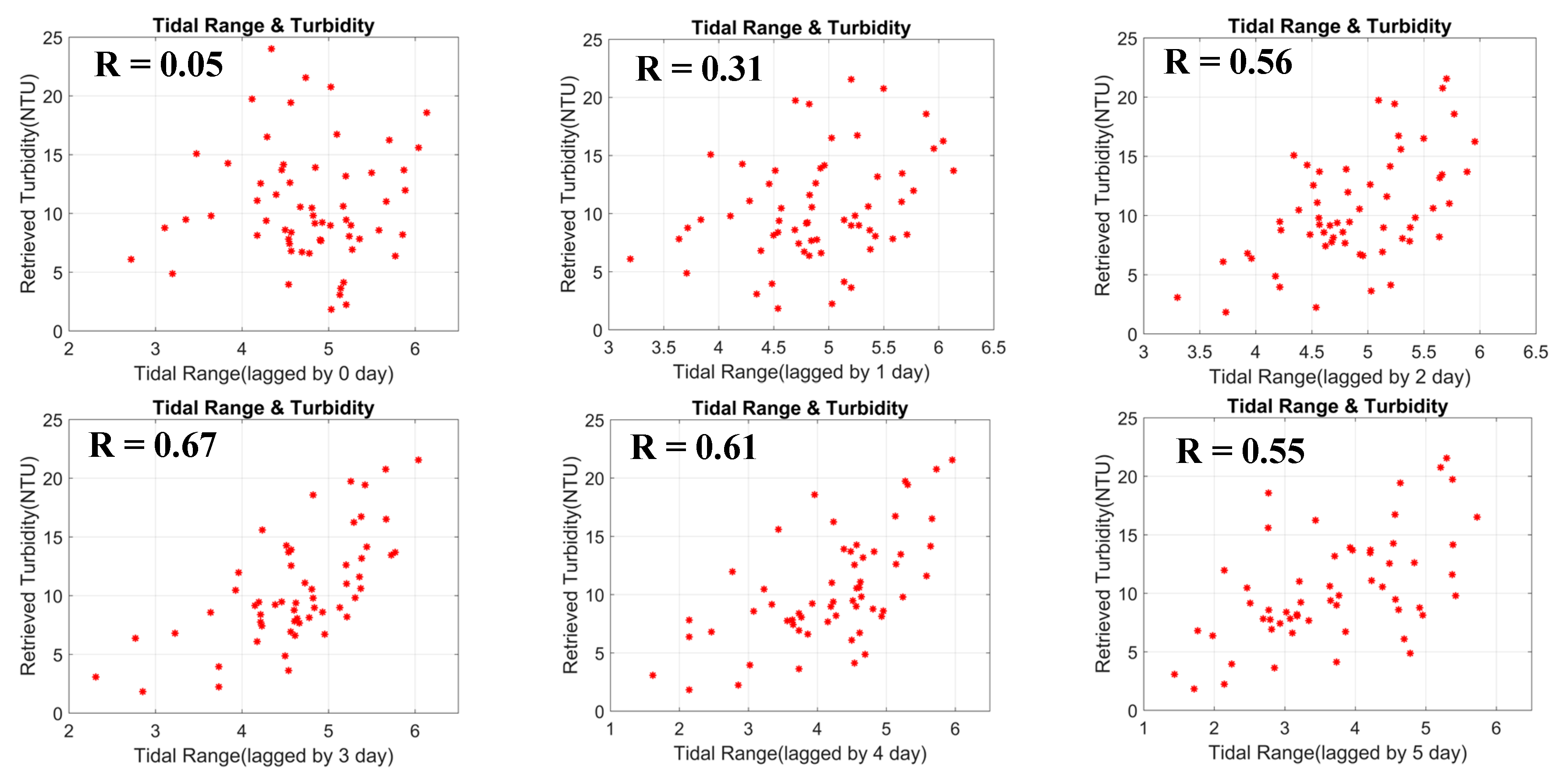
3.2. The Effect of Spring and Neap Tides on Turbidity Variation

Tide is the dominant factor influencing the sediment dynamics and mixing in Darwin Harbour. During the spring tide, the tidal range can exceed 7 m, whereas during the neap tide the tidal range is typically around 2.5 m [43]. In addition, according to measurements at the IMOS station, the peak current velocity can reach to 2 m s⁻¹. The large tidal variation suggests that the hydrodynamics in Darwin Harbour is largely impacted by the spring and neap tides. MODIS data at low water level during the spring and neap tides in the dry season were composited to analyze the influence of tidal range and current on the turbidity in Darwin Harbour. The number of MODIS passes used to retrieve turbidity is shown in

Table 4. Number of MODIS passes with low cloud coverage used to calculate the mean turbidity at low water level during the spring and neap tides in dry seasons.

	2013	2014	2015	2016	2017
Spring	19	32	25	23	26
Neap	28	27	27	27	17

.

Figure 9 shows the turbidity patterns during spring and neap tide. The spatial extent of the TMZ during spring tide was larger than that during the neap tide, especially for the inner harbour, river mouths, and coastal area near Charles Point. A strong eddy was formed near Nightcliff and East Point, due to the larger tidal range and current velocity during the spring tide [37], and a large amount of sediment was trapped, forming a TMZ (Figure 9). According to Li [27], the dredging disposal materials can be advected to the east coast in the outer harbour and be trapped by the eddies. In contrast, in neap tide, the TMZ formed by eddies near Nightcliff and East Point was not as distinct as during the neap tides.

Figure 10 shows the turbidity pattern along transect 1 at low water during the neap and spring tides. In general, turbidity variation during spring and neap tide is significant (p-value < 0.01): turbidity during the spring tide was much higher than that in the neap tide (Figure 10). During the spring tide, the turbidity in Darwin Harbour was about 6 NTU, whereas, during the neap tide, the turbidity was about 3 NTU. During the spring tide, the larger tidal range and strong currents can induce strong vertical mixing and cause large amounts of sediment to be resuspended compared with that during the neap tide, making the turbidity higher [4,37,44,45,46].

Tide is the dominant factor for hydrodynamics and sediment transport in Darwin Harbour [25,36,37,43]. To quantify the influence of the spring–neap tide on turbidity in Darwin Harbour, the correlation between turbidity and tidal range is shown in Figure 11. The tidal range is the daily averaged vertical difference between the high tide and the succeeding low tide. According to van Senden et al. [43], tides have a lagging effect on turbidity. In particular, they found that a lag of one day between the tidal range and turbidity had a strong relationship near Charles Point, based on two periods of measurements (May to August 2013 and January 2010 to January 2011).

Figure 11 shows the relationship between MODIS-retrieved turbidity and tidal range during the dry seasons of 2013–2016 using just the data during low water. Turbidity reached a maximum when the tidal range was largest with a lag of three days (R = 0.67). In contrast to the results of van Senden et al. [43], the one-day lagged tidal range did not have a good relationship with turbidity (R = 0.31), This difference may be caused by water depth. According to Gao et al. [39], water depth can contribute to the lag effect of tidal range and currents on turbidity variation. For a greater depth, it takes longer for the bottom sediment to be suspended to the sea surface. Turbidity sensors used in the study of van Senden et al. [43] were located 1 m above the seabed whereas the MODIS retrieved turbidity is at the ocean surface. The time for bottom suspended sediment to reach the ocean surface where it is detectable by MODIS is likely longer than the time to reach the turbidity sensors of van Senden et al. [43], resulting in a longer lag time for this study.

The high turbidity in spring tide and strong relationship between tidal range and turbidity indicated that spring–neap tide is a key factor influencing the turbidity pattern in Darwin Harbour.

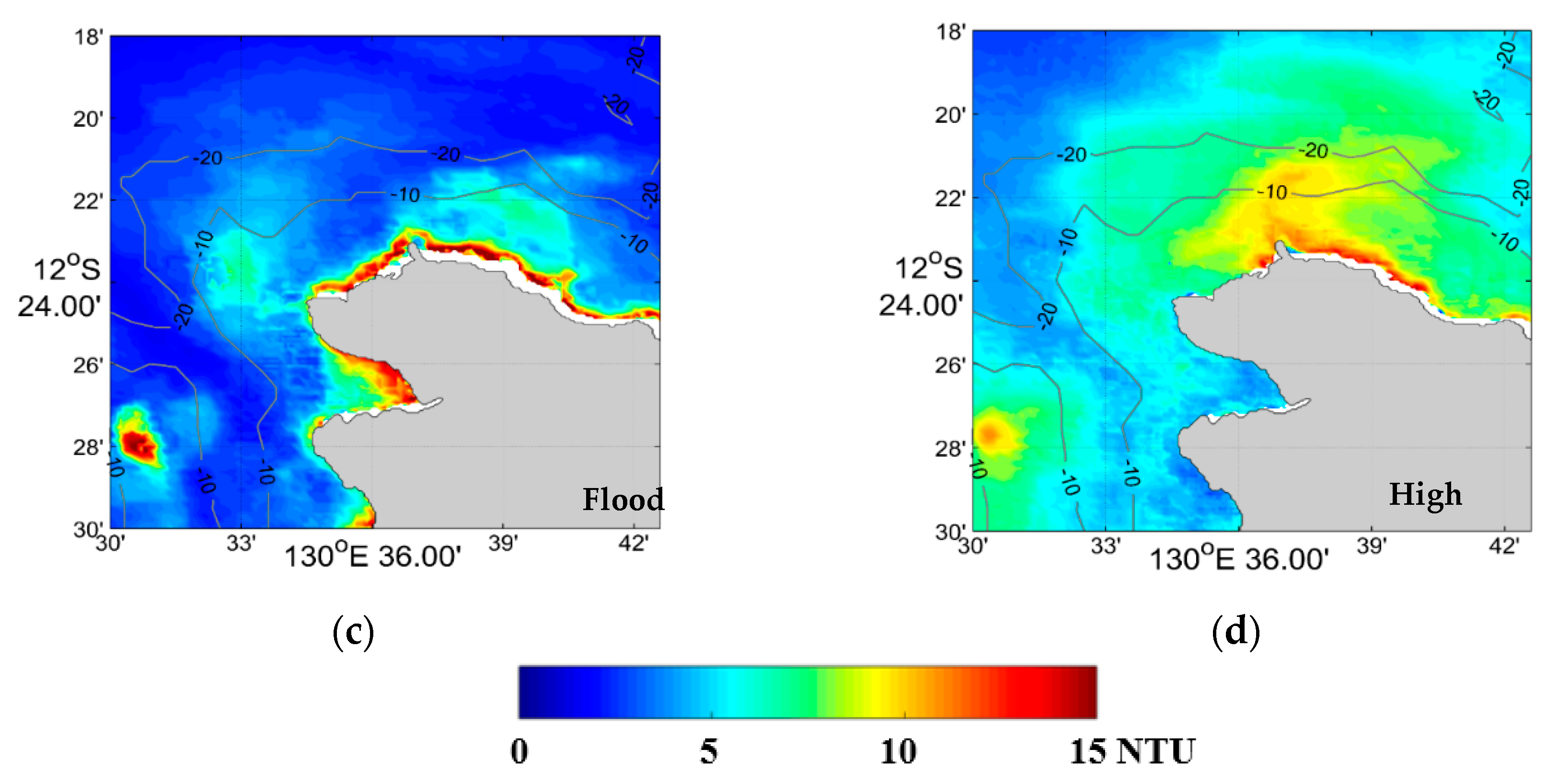
3.3. Intra-Tidal Variation of Turbidity in Darwin Harbour

Darwin Harbour is a semidiurnal macro-tidal area. The highest astronomical tide recorded in Darwin Harbour is 8 m [36]. As discussed in Section 3.2., the spring–neap tides influence the turbidity in Darwin Harbour. It is likely that the diurnal tidal current will also influence the magnitude and distribution of turbidity. To further investigate intra-tidal variation of turbidity in Darwin Harbour, MODIS passes in dry seasons, during spring tides from 2013 to 2017, were chosen for analysis. Using water elevation data at the IMOS station, time averaged turbidity figures were grouped into four phases: ebb tide, low water level, flood tide, and high water level. The number of MODIS passes in each phase is shown in

Table 5. Number of MODIS passes for each phase during the spring tide in the dry season, used to retrieve the turbidity.

	2013	2014	2015	2016	2017
Ebb tide	30	37	34	22	20
Low water level	19	32	25	23	26
Flood tide	6	7	9	4	4
High water level	24	15	13	13	14

. Because there are fewer passes for the flood tide, the low data density results in higher uncertainty for that phase of the diurnal cycle.

The intra-tidal variation of turbidity is shown in Figure 12, Figure 13 and Figure 14. There is a significant variation (p-value < 0.01) in turbidity through the tidal cycle with higher turbidity during the ebb tide and low water level and lower turbidity during flood tide and high water level.

The turbidity is always highest during the ebb tide with two turbidity peaks along transect 1: the first in the upper stream in the inner harbour; and the second in the outer harbour near the mouth of the channel. In the inner harbour, the turbidity is 6–8 NTU in most areas, and reaches 9 NTU near the mouths of rivers. The strong ebb tide resuspends fine sediment near the seabed, increasing the turbidity. In the outer harbour, the effect of eddies near Nightcliff and high current velocity in the mouth of the channel results in a second peak in turbidity along transect 1. Turbidity near the west coast is also high, reaching 11 NTU near Charles Point, due to the resuspension of turbidity by the strong ebb tide.

During the low water level, the turbidity along transect 1 is slightly lower than during the ebb tide and it drops slowly from the inner to outer harbour. This is because after the peak ebb tide, the tidal current weakens and the suspended sediment begins to settle until low slack water is reached, resulting in the decline of turbidity at the sea surface.

The turbidity is lowest during the flood tide and the TMZ is the smallest of the four phases in Darwin Harbour. During this period, a large volume of low turbidity seawater offshore is advected into Darwin Harbour and the water elevation increases, so that surface turbidity is decreased because of dilution by the influxing water [37]. This case is similar to the study of Yalu River Estuary [4] where the authors found that SSC at flood tide was lower than that in ebb tide. Turbidity decreases slowly from the estuary to the main water body in the inner harbour and increases to more than 4 NTU in the mouth of the channel, due to resuspension of sediment by strong tidal currents, similar to the ebb tide process.

At high water level, the turbidity value along transect 1 and in the coastal region near Charles Point, is higher than during the flood tide, which may be due to resuspended sediment near the sea bottom being gradually mixed to the surface during the post peak flood current, increasing the surface turbidity.

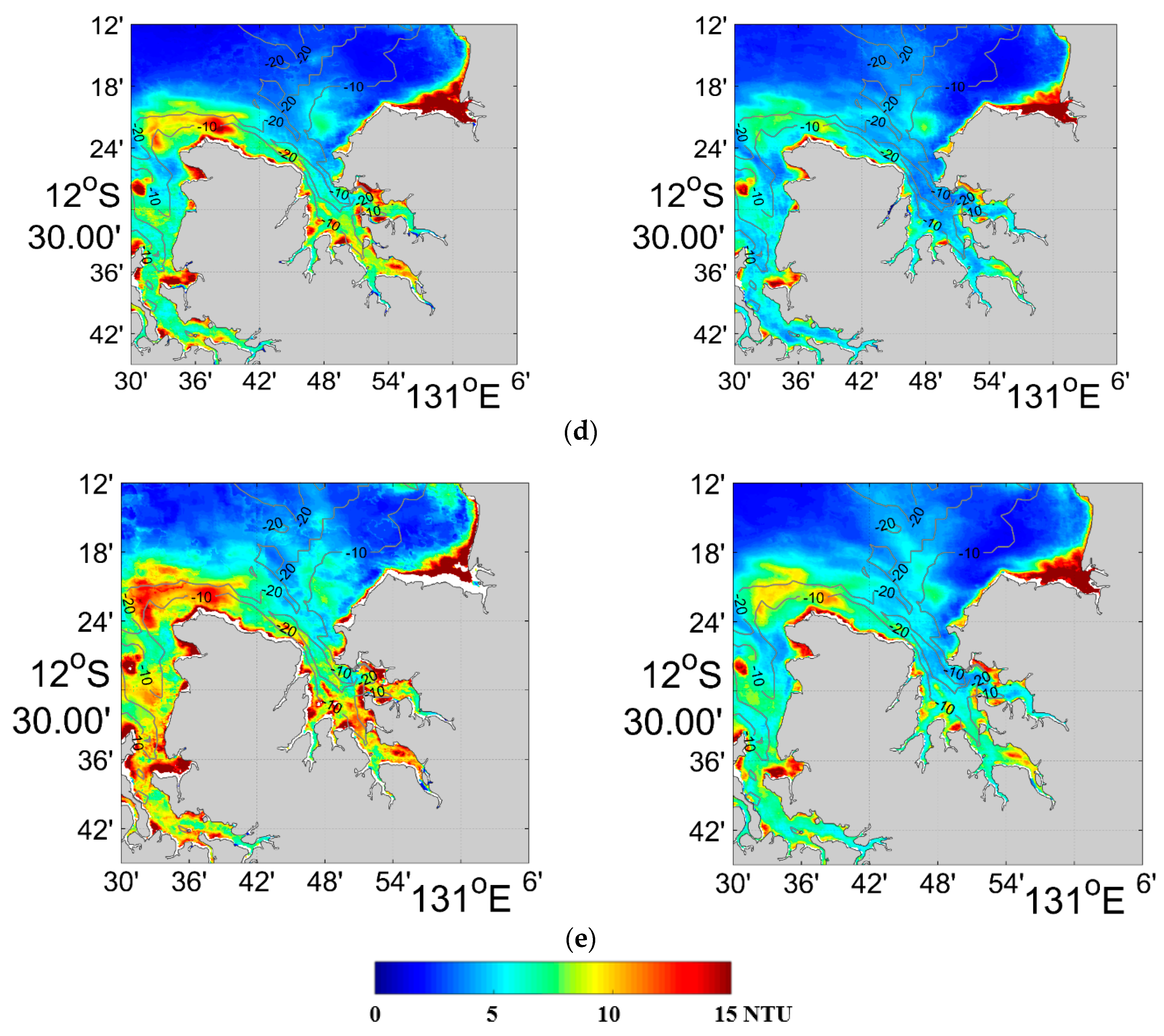
3.4. TMZ near Nightcliff and East Point, and Near Charles Point

According to Li et al. [37], numerical experiments show that the turbid zone is formed by the headland and it disappears when the headland is removed from the model domain. Eddies forming near East point and Nightcliff trap large amounts of suspended sediment and form a high turbid zone.

The MODIS retrieved turbidity show that there is a nearshore TMZ near Charles Point (Area A) during all four phases of the tidal cycle and an offshore TMZ west of Charles Point (Area B) at low water level during the period of observation, particular in the 2014 dry season (Figure 15) and wet seasons from 2013 to 2017 (Figure 3). In order to investigate the mechanisms that control the formation of the TMZ, the Delft3D model was applied to the study area.

The boundary (red dash line) of the two-dimensional (2D) tidal model is shown in Figure 16 and water elevation obtained by Delft Dashboard from the TPXO 7.2 Global Inverse Tide Model at the boundary was used to drive the current model [47,48]. The calculation time step of the current model is 12 s and the time span is from 1 March to 31 May in 2013.

Two cases (flood tide at 05:30 p.m. (local time) on 28 May, ebb tide at 11:30 p.m. (local time) on 28 May 2013) were chosen to show tidal current velocity and direction, convergence, and divergence. The modelling results of the two cases are shown in Figure 17 and validated against current data from the IMOS station in Figure 18. Figure 18 shows a reasonable model data comparison for the depth-averaged tidal current, with correlation coefficients reaching 0.88 and 0.96 for the current speed and direction, respectively. According to the model results, there were two convergence zones at ebb tide (one nearshore near Charles Point (NCP 1), one offshore in the west of Charles Point (WCP 1)) and one convergence zone near Charles Point (NCP 2) at flood tide (Figure 17). The flood tide nearshore convergence area was closer to Charles Point compared with the ebb tide convergence. These convergence zones closely match with the TMZ areas A and B shown in Figure 15. This suggests that the formation of TMZs near Charles Point may be formed by tidal current convergence, similar to Byun and Wang [49] in their study of sediment transport in Mokpo Harbour in Korea.

However, the convergence zone near area B during the ebb tide in Figure 15 became divergent during the flood tide. During this period, the suspended sediment was dispersed and the TMZ at area B disappeared during the flood tide.

4. Conclusions

In this study, band 1 reflectance data from the MODIS product MYD09GQ and MOD09GQ were used to retrieve surface turbidity in Darwin Harbour and adjacent coastal regions for the period from 1 November 2012 to 31 October 2017. The retrievals were used to investigate the variability of turbidity in Darwin Harbour on seasonal, spring–neap cycle and intra-tidal scales.

The turbidity pattern showed clear seasonal variability: higher turbidity during the wet season and lower turbidity during the dry season. The TMZ, which was limited to the mouth of rivers and nearshore areas, was smaller in the dry season compared with that during the wet season. Although discharges of the Blackmore and Elizabeth Rivers during the wet season was much higher than that during the dry season, the river discharge did not show significant impact on the turbidity in Darwin Harbour. In contrast, seasonal wind-driven waves seemed to be the main factor dominating seasonal variation of surface turbidity in Darwin Harbour. The correlation between surface turbidity and wind velocity and significant wave height indicated that high turbidity often corresponded to strong wind waves. The re-suspension of suspended sediment caused by strong waves in Darwin Harbour made the surface turbidity higher during the wet season. In the spring–neap tide cycle, the turbidity in Darwin Harbour showed considerable variation. During the spring tide, the turbidity was much higher and the TMZ was larger than that during the neap tide. The strong relationship between tidal range and turbidity in Darwin Harbour suggested that the tide was the dominant factor controlling turbidity in Darwin Harbour. The turbidity at different tidal phases also showed variability. Turbidity was always higher at low water level and ebb tide, similar to the results of numerical modelling of Li et al. [37]. The effect of tidal re-suspension and advection on turbidity intra-tidal variation was identified.

The study also suggested that the dredging activities in Darwin Harbour in 2013 and 2014 wet season caused the formation of a TMZ in East Arm and a TMZ near the offshore disposal ground. Based on the tidal current modelling results, the TMZ near Charles Point was formed by the convergence of tidal currents.

From the above results, it is concluded that the use of MODIS MYD09GQ/MOD09GQ product band 1 reflectance data is a good method to retrieve surface turbidity variation in relatively clear waters in Darwin Harbour. However, the limitations of the data, as well as the complex hydrodynamics in Darwin Harbour (e.g., wave-current interaction) means that further study with a wave-current coupled numerical model is needed to better understand the turbidity patterns and sediment dynamics in Darwin Harbour and adjacent coastal regions.

References

1. Moreno-Madrinan, M.J.; Al-Hamdan, M.Z.; Rickman, D.L.; Muller-Karger, F.E. Using the Surface Reflectance MODIS Terra Product to Estimate Turbidity in Tampa Bay, Florida. Remote Sens. 2010, 2, 2713–2728. [Google Scholar] [CrossRef]
2. Doxaran, D.; Froidefond, J.; Castaing, P.; Babin, M. Dynamics of the turbidity maximum zone in a macrotidal estuary (the Gironde, France): Observations from field and MODIS satellite data. Estuar. Coast. Shelf Sci. 2009, 81, 321–332. [Google Scholar] [CrossRef]
3. Petus, C.; Chust, G.; Gohin, F.; Doxaran, D.; Froidefond, J.; Sagarminaga, Y. Estimating turbidity and total suspended matter in the Adour River plume (South Bay of Biscay) using MODIS 250-m imagery. Cont. Shelf Res. 2010, 30, 379–392. [Google Scholar] [CrossRef]
4. Cheng, Z.; Wang, X.H.; Paull, D.; Gao, J. Application of the Geostationary Ocean Color Imager to Mapping the Diurnal and Seasonal Variability of Surface Suspended Matter in a Macro-Tidal Estuary. Remote Sens. 2016, 8, 244. [Google Scholar] [CrossRef]
5. Wang, Z.; Qiao, L.; Wang, Y. Progress on Retrieval Models of Suspended Sediment Concentration from Satellite Images in the Eastern China Seas. Acta Sedimentol. Sin. 2016, 34, 292–301. (In Chinese) [Google Scholar]
6. Doxaran, D.; Froidefond, J.; Castaing, P. Remote-sensing reflectance of turbid sediment-dominated waters Reduction of sediment type variations and changing illumination conditions effects by use of reflectance ratios. Appl. Opt. 2003, 42, 2623–2632. [Google Scholar] [CrossRef] [PubMed]
7. Vos, R.J.; Hakvoort, J.H.M.; Jordans, R.W.J.; Ibelings, B.W. Multiplatform optical monitoring of eutrophication in temporally and spatially variable lakes. Sci. Total Environ. 2003, 312, 221–243. [Google Scholar] [CrossRef]
8. Warrick, J.A.; Mertes, L.A.K.; Siegel, D.A.; Mackenzie, C. Estimating suspended sediment concentrations in turbid coastal waters of the Santa Barbara Channel with SeaWiFS. Int. J. Remote Sens. 2004, 25, 1995–2002. [Google Scholar] [CrossRef]
9. Fettweis, M.; Nechad, B.; Van den Eynde, D. An estimate of the suspended particulate matter (SPM) transport in the southern North Sea using SeaWiFS images, in situ measurements and numerical model results. Cont. Shelf Res. 2007, 27, 1568–1583. [Google Scholar] [CrossRef] [Green Version]
10. Miller, R.L.; McKee, B.A. Using MODIS Terra 250 m imagery to map concentrations of total suspended matter in coastal waters. Remote Sens. Environ. 2004, 93, 259–266. [Google Scholar] [CrossRef] [Green Version]
11. Chen, Z.; Hu, C.; Muller-Karger, F. Monitoring turbidity in Tampa Bay using MODIS/Aqua 250-m imagery. Remote Sens. Environ. 2007, 109, 207–220. [Google Scholar] [CrossRef]
12. Petus, C.; Marieu, V.; Novoa, S.; Chust, G.; Bruneau, N.; Froidefond, J. Monitoring spatio-temporal variability of the Adour River turbid plume (Bay of Biscay, France) with MODIS 250-m imagery. Cont. Shelf Res. 2014, 74, 35–49. [Google Scholar] [CrossRef] [Green Version]
13. Chen, S.; Han, L.; Chen, X.; Li, D.; Sun, L.; Li, Y. Estimating wide range Total Suspended Solids concentrations from MODIS 250-m imageries: An improved method. ISPRS J. Photogramm. 2015, 99, 58–69. [Google Scholar] [CrossRef]
14. Mertes, L.A.K.; Smith, M.O.; Adams, J.B. Estimating suspended sediment concentrations in surface waters of the Amazon River wetlands from Landsat images. Remote Sens. Environ. 1993, 43, 281–301. [Google Scholar] [CrossRef]
15. Zhou, W.; Wang, S.; Zhou, Y.; Troy, A. Mapping the concentrations of total suspended matter in Lake Taihu, China, using Landsat-5 TM data. Int. J. Remote Sens. 2006, 27, 1177–1191. [Google Scholar] [CrossRef]
16. Kallio, K.; Attila, J.; Härmä, P.; Koponen, S.; Pulliainen, J.; Hyytiäinen, U.; Pyhälahti, T. Landsat ETM+ Images in the Estimation of Seasonal Lake Water Quality in Boreal River Basins. Environ. Manag. 2008, 42, 511–522. [Google Scholar] [CrossRef] [PubMed]
17. Kulkarni, A. Water Quality Retrieval from Landsat TM Imagery. Procedia Comput. Sci. 2011, 6, 475–480. [Google Scholar] [CrossRef]
18. Vanhellemont, Q.; Ruddick, K. Turbid wakes associated with offshore wind turbines observed with Landsat 8. Remote Sens. Environ. 2014, 145, 105–115. [Google Scholar] [CrossRef]
19. Ruddick, K.; Vanhellemont, Q.; Yan, J.; Neukermans, G.; Wei, G.; Shang, S. Variability of suspended particulate matter in the Bohai Sea from the geostationary Ocean Color Imager (GOCI). Ocean Sci. J. 2012, 47, 331–345. [Google Scholar] [CrossRef]
20. Lyu, H.; Zhang, J.; Zha, G.; Wang, Q.; Li, Y. Developing a two-step retrieval method for estimating total suspended solid concentration in Chinese turbid inland lakes using Geostationary Ocean Colour Imager (GOCI) imagery. Int. J. Remote Sens. 2015, 36, 1385–1405. [Google Scholar] [CrossRef]
21. Moore, G.F.; Aiken, J.; Lavender, S.J. The atmospheric correction of water colour and the quantitative retrieval of suspended particulate matter in Case II waters: Application to MERIS. Int. J. Remote Sens. 1999, 20, 1713–1733. [Google Scholar] [CrossRef]
22. Shen, F.; Verhoef, W.; Zhou, Y.; Salama, M.S.; Liu, X. Satellite Estimates of Wide-Range Suspended Sediment Concentrations in Changjiang (Yangtze) Estuary Using MERIS Data. Estuar. Coast. 2010, 33, 1420–1429. [Google Scholar] [CrossRef] [Green Version]
23. Fischer, A.; Pang, D.; Kidd, I.; Moreno-Madriñán, M. Spatio-Temporal Variability in a Turbid and Dynamic Tidal Estuarine Environment (Tasmania, Australia): An Assessment of MODIS Band 1 Reflectance. ISPRS Int. J. Geo-Inf. 2017, 6, 320. [Google Scholar] [CrossRef]
24. Hamidi, S.; Hosseiny, H.; Ekhtari, N.; Khazaei, B. Using MODIS remote sensing data for mapping the spatio-temporal variability of water quality and river turbid plume. J. Coast. Conserv. 2017, 21, 939–950. [Google Scholar] [CrossRef]
25. Andutta, F.P.; Wang, X.H.; Li, L.; Williams, D. Hydrodynamics and Sediment Transport in a Macro-Tidal Estuary: Darwin Harbour, Australia; Springer: Dordrecht, The Netherlands, 2013; pp. 111–129. [Google Scholar]
26. Wang, X.H.; Andutta, F.P. Sediment transport dynamics in ports, estuaries and other coastal environments. In Sediment Transport; Manning, A.J., Ed.; Intech: London, UK, 2012; pp. 3–35. ISBN 980-953-307-557-5. [Google Scholar]
27. Li, L. Modelling the Tidal and Sediment Dynamics in Darwin Harbour, Northern Territory, Australia. Ph.D. Thesis, The University of New South Wales, Canberra, Australia, 2013. [Google Scholar]
28. Fortune, J. The Grainsize and Heavy Metal Content of Sediment in Darwin Harbour; Report No.: 14/2006D; Aquatic Health Unit, Environmental Protection Agency, Department of Natural Resources, Environment and the Arts: Darwin, NT, USA, 2016; 74p. [Google Scholar]
29. McKinnon, A.D.; Smit, N.; Townsend, S.; Duggan, S. Darwin Harbour: Water quality and ecosystem structure in a tropical harbour in the early stages of urban development. In The Environment in Asia Pacific Harbour; Wolanski, E., Ed.; Springer: Dordrecht, The Netherlands, 2006; pp. 433–459. [Google Scholar]
30. Padovan, A. The Water Quality of Darwin Harbour October 1990-November 1991; Water Quality Branch, Water Resources Division, Department of Lands, Planning and Environment: Darwin, Australia, 1997. [Google Scholar]
31. Nechad, B.; Ruddick, K.G.; Park, Y. Calibration and validation of a generic multisensor algorithm for mapping of total suspended matter in turbid waters. Remote Sens. Environ. 2010, 114, 854–866. [Google Scholar] [CrossRef]
32. Dorji, P.; Fearns, P.; Broomhall, M. A Semi-Analytic Model for Estimating Total Suspended Sediment Concentration in Turbid Coastal Waters of Northern Western Australia Using MODIS-Aqua 250 m Data. Remote Sens. 2016, 8, 556. [Google Scholar] [CrossRef]
33. Dorji, P.; Fearns, P. Impact of the spatial resolution of satellite remote sensing sensors in the quantification of total suspended sediment concentration: A case study in turbid waters of Northern Western Australia. PLoS ONE 2017, 12, e0175042. [Google Scholar] [CrossRef] [PubMed]
34. Joshi, I.D.; D’Sa, E.J.; Osburn, C.L.; Bianchi, T.S. Turbidity in Apalachicola Bay, Florida from Landsat 5 TM and Field Data: Seasonal Patterns and Response to Extreme Events. Remote Sens. 2017, 9, 367. [Google Scholar] [CrossRef]
35. Carballo, R.; Iglesias, G.; Castro, A. Residual circulation in the Ría de Muros (NW Spain): A 3D numerical model study. J. Mar. Syst. 2009, 75, 116–130. [Google Scholar] [CrossRef]
36. Williams, D.; Wolanski, E.; Spagnol, S. Hydrodynamics of Darwin Harbour. In The Environment in Asia Pacific Harbours; Wolanski, E., Ed.; Springer: Dordrecht, The Netherlands, 2006; pp. 461–476. [Google Scholar]
37. Li, L.; Wang, X.H.; Andutta, F.P.; Williams, D. Effects of mangroves and tidal flats on suspended-sediment dynamics: Observational and numerical study of Darwin Harbour, Australia. J. Geophys. Res. 2014, 119, 5854–5873. [Google Scholar] [CrossRef] [Green Version]
38. Green, M.O.; Coco, G. Review of wave-driven sediment resuspension and transport in estuaries. Rev. Geophys. 2014, 52, 77–117. [Google Scholar] [CrossRef] [Green Version]
39. Gao, A.; Zhao, H.; Yang, S.; Dai, S.; Chen, S.; Li, P. Seasonal and Tidal Variations in Suspended Sediment Concentration Under the Influence of River Runoff, Tidal Current and Wind Waves. Adv. Mar. Sci. 2008, 26, 44–48. (In Chinese) [Google Scholar]
40. Guillou, N.; Rivier, A.; Chapalain, G.; Gohin, F. The impact of tides and waves on near-surface suspended sediment concentrations in the English Channel. Oceanologia 2017, 59, 28–36. [Google Scholar] [CrossRef]
41. Utne-Palm, A. The effect of prey mobility, prey contrast, turbidity and spectral composition on the reaction distance of Gobiusculus flavescens to its planktonic prey. J. Fish Biol. 1999, 54, 1244–1258. [Google Scholar] [CrossRef]
42. Wang, X.H.; Pinardi, N. Modeling the dynamics of sediment transport and resuspension in the northern Adriatic Sea. J. Geophys. Res. 2002, 107, 18:1–18:23. [Google Scholar] [CrossRef]
43. Van Senden, D.; Taylor, D.; Branson, P. Realtime turbidity monitoring and modelling for dredge impact assessment in Darwin Harbour. In Proceedings of the Australasian Port and Harbour Conference, Sydney, Australia, 27–29 November 2017; pp. 797–802. [Google Scholar]
44. Allen, G.P.; Salomon, J.C.; Bassoullet, P.; Du Penhoat, Y.; De Grandpré, C. Effects of tides on mixing and suspended sediment transport in macrotidal estuaries. Sediment. Geol. 1980, 26, 69–90. [Google Scholar] [CrossRef]
45. Ramaswamy, V.; Rao, P.S.; Rao, K.H.; Thwin, S.; Rao, N.S.; Raiker, V. Tidal influence on suspended sediment distribution and dispersal in the northern Andaman Sea and Gulf of Martaban. Mar. Geol. 2004, 208, 33–42. [Google Scholar] [CrossRef]
46. Unverricht, D.; Nguyen, T.C.; Heinrich, C.; Szczuciński, W.; Lahajnar, N.; Stattegger, K. Suspended sediment dynamics during the intra-monsoon season in the subaqueous Mekong Delta and adjacent shelf, southern Vietnam. J. Asian Earth Sci. 2014, 79, 509–519. [Google Scholar] [CrossRef]
47. Egbert, G.D.; Erofeeva, S.Y. Efficient inverse modeling of barotropic ocean tides. J. Atmos. Ocean. Technol. 2002, 19, 183–204. [Google Scholar] [CrossRef]
48. Egbert, G.D.; Bennett, A.F.; Foreman, M.G.G. TOPEX/POSEIDON tides estimated using a global inverse model. J. Geophys. Res. 1994, 99, 24821–24852. [Google Scholar] [CrossRef]
49. Byun, D.S.; Wang, X.H. The effect of sediment stratification on tidal dynamics and sediment transport patterns. J. Geophys. Res. 2005, 110, C3. [Google Scholar] [CrossRef]
Figure 1. Map of Darwin Harbour and the adjacent coastal region. The red dot shows the location of the Integrated Marine Observing System station (IMOS). Blue dots show the positions of selected stations A and B. The line between P1 and P2 shows the location of transect 1. The red line between Mandorah Point and East Point is the boundary between the outer and inner harbour.
Remotesensing 10 00997 g001
Figure 2. (a) The calibrated SASM (Equations (2) and (3)) using regression analysis between in situ turbidity and x; (b) comparisons between measured turbidity at the IMOS station and the MODIS retrieved surface turbidity.
Remotesensing 10 00997 g002
Figure 3. MODIS retrieved seasonally averaged turbidity for the low water spring tide in Darwin Harbour for the wet season (left) and dry season (right) during: (a) 2013; (b) 2014; (c) 2015; (d) 2016; and (e) 2017. The dredging offshore disposal area is shown by the red box.
Remotesensing 10 00997 g003aRemotesensing 10 00997 g003b
Figure 4. The turbidity with standard deviation in the wet and dry seasons at (a) A station; and (b) B station.
Remotesensing 10 00997 g004
Figure 5. Mean seasonal turbidity along transect 1 (~36 km) in: (a) 2013; (b) 2014; (c) 2015; (d) 2016; and (e) 2017. The standard deviation is indicated by the error bars.
Remotesensing 10 00997 g005aRemotesensing 10 00997 g005b
Figure 6. Monthly river discharge of Blackmore River (Station G8150098), Berry Creek (Station 8150028), and Elizabeth River (Station G8150018).
Remotesensing 10 00997 g006
Figure 7. Wind speed and direction roses (e.g., direction with a value of 315 means wind comes from the northwest) during the wet season (left) and dry season (right) in: (a) 2013; (b) 2014; (c) 2015; (d) 2016; and (e) 2017.
Remotesensing 10 00997 g007aRemotesensing 10 00997 g007b
Figure 8. The relationship between the MODIS-Aqua retrieved turbidity at the IMOS station during the low water spring tide and corresponding significant waves height and wind speed for cloudless days during the observation period from 2013 to 2017.
Remotesensing 10 00997 g008
Figure 9. MODIS retrieved averaged turbidity for low water spring (left) and neap (right) tide in the dry season during: (a) 2013; (b) 2014; (c) 2015; (d) 2016; and (e) 2017. The location of the TMZ formed by eddies is shown by the red box.
Remotesensing 10 00997 g009aRemotesensing 10 00997 g009b
Figure 10. Mean retrieved turbidity with standard deviation along transect 1 at low water spring and neap tide in the dry season during: (a) 2013; (b) 2014; (c) 2015; (d) 2016; and (e) 2017.
Remotesensing 10 00997 g010
Figure 11. The relationship between retrieved turbidity at low water level and the tidal range at Station A.
Remotesensing 10 00997 g011
Figure 12. MODIS-retrieved averaged turbidity during spring tide in the dry season during: (a) 2013; (b) 2014; (c) 2015; (d) 2016; and (e) 2017.
Remotesensing 10 00997 g012
Figure 13. Time averaged retrieved turbidity for each phase along transect 1 during: (a) 2013; (b) 2014; (c) 2015; (d) 2016; and (e) 2017.
Remotesensing 10 00997 g013
Figure 14. Turbidity at stations A and B for each phase during the spring tide during: (a) 2013; (b) 2014; (c) 2015; (d) 2016; and (e) 2017. The standard deviation is indicated by the error bars.
Remotesensing 10 00997 g014
Figure 15. Location of the TMZ near Charles Point (Area A) and the TMZ in the northwest of Charles Point (Area B) during the four tidal phases (a) ebb tide; (b) low water level; (c) flood tide; and (d) high water level during the 2014 dry season.
Remotesensing 10 00997 g015aRemotesensing 10 00997 g015b
Figure 16. The 2D current model domain and open boundary for the water elevation boundary (red dash line).
Remotesensing 10 00997 g016
Figure 17. Tidal current convergence and divergence (− 𝛻 V = u x + ν y , positive value: convergence, negative value: divergence) at flood and ebb tide (05:30 p.m. on 28 May, 11:30 p.m. on 28 May 2013), respectively.
Remotesensing 10 00997 g017
Figure 18. The Delft 3D modelling tidal depth averaged current velocity and direction with current data from IMOS station from 00:00 a.m. 28 May to 10:00 p.m. 30 May 2013.
Remotesensing 10 00997 g018