Assessment of Root Zone Soil Moisture Estimations from SMAP, SMOS and MODIS Observations

Abstract

In this study, six satellite-based root zone soil moisture (RZSM) estimates from March 2015 to December 2016 were evaluated both temporally and spatially. The first two were the Soil Moisture Active Passive (SMAP) and the Soil Moisture and Ocean Salinity (SMOS) L4 RZSM products. The other four were obtained through the Soil Water Index (SWI) approach, which embedded surface soil moisture (SSM). The SMOS-Barcelona Expert Center (BEC) L4 SSM product and the apparent thermal inertia (ATI)-derived SSM from the Moderate Resolution Imaging Spectroradiometer (MODIS) data were used as SSM datasets. In the temporal analysis, the RZSM estimates were compared to in situ RZSM from 14 stations of the Soil Moisture Measurements Station Network of the University of Salamanca (REMEDHUS). Regarding the spatial assessment, the resulting RZSM maps of the Iberian Peninsula were compared between them. All RZSM values followed the temporal evolution of the ground-based measurements well, although SMOS and MODIS showed underestimation while SMAP displayed overestimation. The good results obtained from MODIS ATI are notable, notwithstanding they were not estimated through microwave radiometry. A very high agreement was found in terms of spatial patterns for the whole Iberian Peninsula except for the extreme north area, which is dominated by high mountains and dense forests.

1. Introduction

L-band radiometry is the most established technique for remotely measuring soil moisture. Currently, there are two L-band missions in orbit specifically designed to globally monitor soil moisture: the Soil Moisture and Ocean Salinity (SMOS) and the Soil Moisture Active Passive (SMAP). SMOS, launched in 2009 by the European Space Agency (ESA), uses a synthetic aperture radiometer with a spatial resolution of ~35–50 km to provide global soil moisture maps every three days [1]. The Centre Aval de Traitement des Données SMOS (CATDS) provides several soil moisture products (L2, L3, and L4), which are processed with the algorithms developed by the Centre d’Etudes Spatiales de la Biosphere (CESBIO). In 2015, the National Aeronautics and Space Administration (NASA) launched SMAP. It currently employs a real aperture radiometer with ~40 km resolution to retrieve soil moisture maps with a three-day revisit time [2].

While these remote sensing sensors provide soil moisture data at coarse spatial resolutions, a growing number of applications require knowledge of soil moisture at regional or local scales (from a few kilometers down to several meters). To overcome this challenge, some soil moisture disaggregation approaches have been developed, such as those based on the synergy of passive microwaves with ancillary optical visible/infrared (VIS/IR) [3,4,5,6] or active data [7]. Optical data have also been used to indirectly estimate soil moisture [8]. For instance, methods based on apparent thermal inertia (ATI) to estimate soil moisture rely upon the fact that wet soils have a higher thermal inertia and a lower temperature fluctuation than dry soils. When soil moisture increases, ATI proportionally increases as well, and there is a short-term reduction in the diurnal land surface temperature (LST) range [9,10,11,12,13].

A main drawback of the L-band observations is that although they have larger penetration than those at higher microwaves (S-, C-, X-, or K-bands), they explore approximately 0–5 cm of the topsoil layer, sensing only surface soil moisture (SSM). However, an increasing number of hydrological and agricultural applications require root zone soil moisture (RZSM) information from the soil profile (0–1 m depth), where plant roots develop [14,15]. Additionally, the SSM may not have significant influence in the soil water availability for plants and crops. For this reason, the RZSM is expected to better reflect the actual soil water content storage of the unsaturated zone than the SSM.

There are several methods for obtaining RZSM. One method comprises in situ soil moisture measurements made at the root zone using probes installed either at a specific depth required or along the whole soil profile. In this regard, although neutron attenuation probes were extensively used in the past, sensors based on the soil dielectric constant—capacitance, Frequency Domain Reflectivity (FDR) and Time Domain Reflectivity (TDR) probes—are now being employed in many networks worldwide [16]. Another method involves using cosmic-ray soil moisture probes. These innovative and noninvasive sensors have been implemented in the Cosmic-ray Soil Moisture Observing System (COSMOS) network [17,18]. The cosmic-ray sensors are placed above the soil surface, but its effective soil measurement depth varies from 12 cm for wet soils to 76 cm for dry soils [19]. Nevertheless, only a limited number of current networks of the International Soil Moisture Network (ISMN) provide RZSM compared to the great amount that provide SSM. Another method relies on the use of Ground Penetration Radar (GPR) measurements. In this case, the GPR sensor can be mounted on a vehicle close the soil surface or an airplane to measure soil moisture during experimental field campaigns. The GPR does not require direct contact with the soil, but its signal can penetrate from one meter to several tens of meters [20]. The last method consists of estimating RZSM through more or less complex models that have this variable as the output.

The models used to estimate RZSM can be classified into two main groups: the so-called land-surface models and the hydrological models. They differ in the detail of description of processes that are taken into account, the parameter estimation approaches, and the spatiotemporal resolutions. Land-surface models describe the vertical exchanges of heat, water, and carbon considering the land-atmosphere couplings and are globally applied. Hydrological models are instead more focused on water resources, are traditionally applied at the basin level, and usually have many parameters that need to be calibrated or estimated regionally [21]. Different data assimilation techniques are used in the two cases to incorporate SSM to them [22,23,24]. Originally, the assimilated SSM data to estimate RZSM had been measured in situ [25,26], but a variety of satellite SSM data have been assimilated in the last decade [27,28,29]. In the case of SMAP and SMOS missions, two operational satellite-based RZSM products have recently been developed from the assimilation of SSM measurements into their respective land-surface models [30,31].

The Soil Water Index (SWI) is one of the most common models used to estimate RZSM through SSM remote sensing [32]. This simple model has been able to successfully obtain RZSM over regions with different climatic and soil conditions. Apart from SSM measurements, the SWI requires only an input exponential parameter (T), which is related to the transfer time of water along the soil profile. The T parameter had been calculated in different ways depending on the application, study area, and sensor used [33]. The SWI has been applied to in situ SSM databases in several studies to obtain field scale RZSM [34,35,36] as well as to active and passive SSM observations to generate several satellite-based RZSM estimates, such as those derived from the European Remote Sensing (ERS) scatterometer [37], the Advanced Scatterometer (ASCAT) [38,39,40], the Advanced Microwave Scanning Radiometer-Earth Observing System (AMSR-E) [39,41], the SMOS [42,43], and the Climate Change Initiative (CCI) soil moisture database [41,44].

The aim of this work was to evaluate six RZSM estimates obtained from SMAP, SMOS, and Moderate Resolution Imaging Spectroradiometer (MODIS) from 31 March 2015 to 31 December 2016. The study period (one year and nine months) is limited at the beginning by the SMAP launch and at the end by the availability of two SMOS soil moisture products—the SMOS-CESBIO L4 RZSM and the SMOS-Barcelona Expert Centre (BEC) L4 SSM. The first two RZSM estimates came from the SMAP and the SMOS-CESBIO L4 RZSM products. The other four RZSM estimates were customized products generated after applying the SWI model to two SSM datasets—the SMOS-BEC L4 SSM and the MODIS ATI-derived SSM—together with two alternatives for calculating the exponential T parameter of the SWI. Presently, some studies devoted to validate SMAP and SMOS RZSM have been published, but none have been made validating both RZSM products at the same network or showing an intercomparison between them over the same study area, including a RZSM estimation based on ATI. Thus, the present work will constitute a novelty within this research line. In this study, all satellite-based RZSM estimates were analyzed both temporarily and spatially. For the temporal analysis, the RZSM estimates were compared against in situ RZSM measurements from 14 stations of the Soil Moisture Measurements Station Network of the University of Salamanca (REMEDHUS). The spatial analysis was based on comparisons of RZSM maps from all the analyzed estimates over the entire Iberian Peninsula (~582,000 km²), an area of contrasting environments in both wet and dry periods.

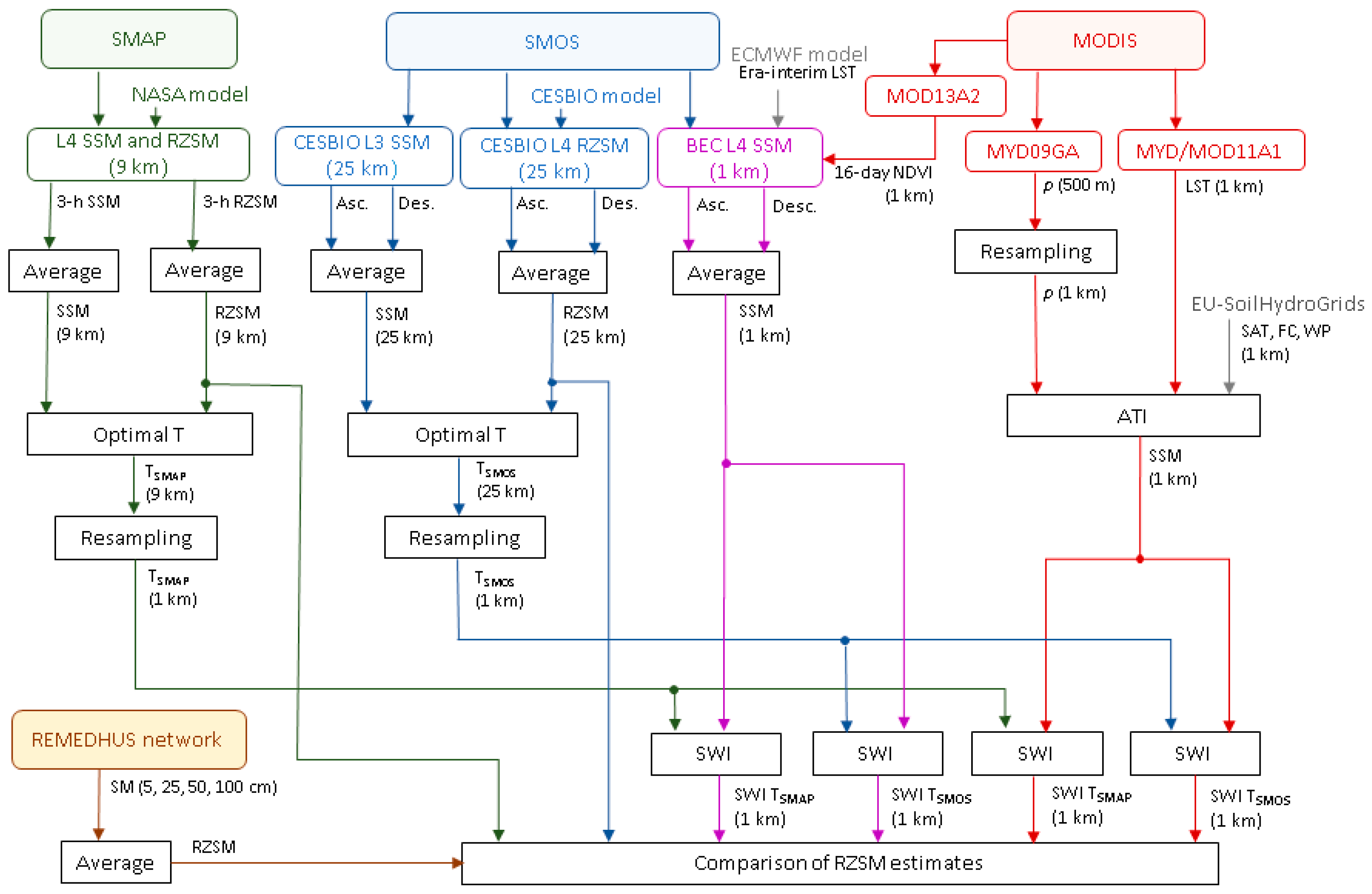
2. Data and Methodology

2.1. REMEDHUS Soil Moisture

REMEDHUS is a soil moisture network located in the central part of the Duero basin in Spain and covering an area of approximately 1300 km² (41.1–41.5°N, 5.1–5.7°W). This region has a continental semiarid Mediterranean climate characterized by a clear water deficit, especially during summer. The location of the network was chosen precisely for these criteria, i.e., to monitor crop behavior under the water-limited conditions and over land covers representative of the region. In REMEDHUS, the main land use is agricultural, with rainfed crops such as cereals, legumes, and vineyards. These crops are adapted to the scarcity of water because most of them are fed only by precipitation, which is approximately 381 mm/year on average [45]. The soils are mainly sandy, leading to a limited water holding capacity.

Two sensor types are installed in REMEDHUS. First, there are 22 stations measuring SSM (0–5 cm) using Hydra Probes (Stevens Water Monitoring, Inc., Portland, OR, USA). Out of the 22 stations, 14 also measure soil moisture along the soil profile using EnviroSMART (Sentek Pty. Ltd., Stepney, SA, Australia) sensors deployed at 25, 50, and 100 cm depths. These depth levels ensure a complete measurement of the soil moisture at the root zone in the area [43].

For the assessment of the ATI-derived SSM, the in situ SSM data provided by all 22 stations in REMEDHUS were used. For the analysis of the RZSM estimates, the soil moisture observations at surface and root zone level from the 14 stations were used. Since the observations are on an hourly basis, soil moisture measurements at each station were first daily averaged. A representative estimate of in situ RZSM was obtained for each station by averaging the daily soil moisture measurements at the different depths (5, 25, 50, and 100 cm).

2.2. SMAP L4 Soil Moisture

Among the variety of SMAP products available, the global SMAP L4 soil moisture geophysical data over a 9-km Equal-Area Scalable Earth (EASE)-2 grid [46] were selected. The SMAP brightness temperature—originally at coarser resolution—was downscaled to 9 km using the Backus-Gilbert optimal interpolation. The SMAP L4 soil moisture was derived by assimilating this brightness temperature into the NASA catchment land-surface model, which interpolates and extrapolates the SMAP observations in time and in space [47]. The NASA model describes the vertical transfer of soil moisture between the surface and the root zone, built on a set of Richard’s equation calculations under unsaturated conditions. This model is driven by observation-based surface meteorological forcing, including precipitation [30].

The SMAP L4 product provides SSM (0–5 cm) and RZSM (0–100 cm) estimations at a 3 h temporal resolution. In this study, the area corresponding to the Iberian Peninsula (34°N–45°N, 11°W–5°E) was clipped from the global SMAP L4 soil moisture maps. The resulting maps of SSM and RZSM were daily averaged.

2.3. SMOS Soil Moisture

2.3.1. SMOS-CESBIO L3 Surface Soil Moisture

The global SMOS L3 SSM product over a 25-km EASE-2 grid was used. The SMOS L3 processor of CESBIO [48] uses the same physically based forward model as the L2 processor [49], with only minor differences that are mainly related to the gridding system. The L3 SSM retrievals are obtained from the SMOS L1C v.620 brightness temperature. On a given day, the L3 algorithm processes several orbits in the same loop. Later, filtering is applied to select the best estimate when several retrievals are available for the same pixel. Therefore, this product is a daily composite of filtered and binned SMOS SSM data [50].

The SMOS-CESBIO L3 SSM is disseminated in separated daily ascending and descending orbits. Similar to the process used for SMAP L4, the area corresponding to the Iberian Peninsula was clipped. Then, a daily average of the ascending and descending orbit maps was applied.

2.3.2. SMOS-CESBIO L4 Root Zone Soil Moisture

Regarding the current SMOS-derived RZSM products, the global SMOS L4 RZSM at 0–1 m depth over a 25-km EASE-2 grid was used. These data were obtained from the SMOS-CESBIO L3 SSM (using a 3-day average SSM) and other ancillary datasets, such as MODIS observations and climate data from the National Centers for Environmental Prediction (NCEP), among others. The RZSM is computed using a double bucket hydrological model, which is applied daily. The CESBIO model has two soil layers (0–40 cm and 40–100 cm). For the first layer, the selected model is the previously mentioned SWI [32,33]. For the second layer, a water balance model based on a linearized Richard’s equation is employed [31].

Since the SMOS-CESBIO L4 RZSM is also distributed separately for daily ascending and descending orbits, the Iberian Peninsula area was clipped from these RZSM maps and a daily average of the ascending and descending orbits was then performed.

2.3.3. SMOS-BEC L4 Surface Soil Moisture

The cloud-free SMOS L4 SSM product—a disaggregated soil moisture at 1 km over the Iberian Peninsula—was used. This product is based on a semi-empirical downscaling approach that combines SMOS and MODIS observations together with data from the European Centre for Medium-Range Weather Forecasts (ECMWF). The product uses a shape-adaptive moving window to integrate the SMOS brightness temperature (L1C v.620) and SSM (L2 v.620) at 25 km, the 16-day Terra MODIS Normalized Difference Vegetation Index (NDVI, MOD13A3 v.5) at 1 km, and the modeled ECMWF Era Retrospective Analysis (ERA)-Interim LST in a linear linking model [51]. The downscaling algorithm is applied separately for daily ascending and descending orbits. As with the previous products, the daily average of ascending and descending data was used.

2.4. MODIS Surface Reflectance and Land Surface Temperature

The daily Aqua MODIS surface reflectance at 500 m (MYD09GA v.6) acquired in bands 1 (620–670 nm), 2 (841–876 nm), 3 (459–479 nm), 4 (545–565 nm), 5 (1230–1250 nm), and 7 (2105–2155 nm) were used. The MODIS reflectance is measured at ground level in the absence of atmospheric scattering or absorption and is already corrected for atmospheric gases, aerosols, and thin cirrus clouds [52]. Regarding the LST, daily Aqua MODIS LST (MYD11A1 v.6) and Terra MODIS LST (MOD11A1 v.6)—both at 1 km spatial resolution—were used. They have an accuracy specification of 1 °C under clear-sky conditions [53].

The three MODIS products are provided into a tile-based sinusoidal projection. The four tiles corresponding to the Iberian Peninsula (h17v04, h17v05, h18v04 and h18v05) were selected. These four tiles of the reflectance maps were first mosaicked. The resulting maps were resampled from the sinusoidal grid to a regular 500 m grid using the nearest neighbor approach. The same processing was applied to the LST but for a regular 1 km grid. The reflectance in all bands was filtered using their corresponding flags (land and highest quality). Finally, the reflectance maps at 500 m were aggregated to the same 1 km grid for the LST using a simple average.

2.5. Estimation of MODIS ATI

The MODIS ATI was computed as the ratio of the daily surface albedo and the diurnal temperature range [10]:

$$ATI=C\frac{1-\alpha }{\Delta LST},$$

(1)

where C is the solar correction factor, α is the broadband albedo and ΔLST corresponds to the diurnal temperature range.

The correction factor C is related to the solar flux and therefore compensates for seasonal variation in solar insolation. This factor was obtained following the expression [10]:

$$C=\sin \phi \sin \delta {(1-{\tan }^2\phi {\tan }^2\delta )}^{1/2}+\cos \phi \cos \delta \mathrm{arcos}(-\tan \phi \tan \delta ),$$

(2)

where $\phi$ corresponds to the latitude and $\delta$ to the solar declination of each pixel for each Julian day of the year.

The broadband albedo can be computed in two different spectral ranges—shortwave and visible in Equations (3) and (4), respectively—from daily Aqua MODIS surface reflectance at 1 km [54]:

$${\alpha }_{\mathrm{shortwave}}=0.160{\rho }_1+0.291{\rho }_2+0.243{\rho }_3+0.116{\rho }_4+0.112{\rho }_5+0.081{\rho }_7-0.0015,$$

(3)

$${\alpha }_{\mathrm{visible}}=0.331{\rho }_1+0.424{\rho }_3+0.246{\rho }_4,$$

(4)

where ${\rho }_1$, ${\rho }_2$, ${\rho }_3,{\rho }_4,{\rho }_5$ and ${\rho }_7$ are reflectance in bands 1, 2, 3, 4, 5 and 7, respectively. These two albedo approaches were analyzed.

The diurnal temperature range can be approximated in four different ways. The first method consists of estimating the LST through time as a sinusoid defined by its amplitude, its average temperature, the angular velocity of Earth, and the phase angle ($\mathsf{\Psi }$) corresponding to the time of daily maximum LST [11,13], which coincides with the time of highest correlation between the LST and soil moisture behavior [55]. MODIS provides up to four observations for each day: Aqua nighttime LST at 1:30 h, Terra daytime LST at 10:30 h, Aqua daytime LST at 13:30 h, and Terra nighttime LST at 22:30 h, local time. These four LST at 1 km were used to compute ΔLST as the solution of the amplitude of the sinusoid by means of the least squares method (ΔLST_4values). In this case, the four LST values are required to derive $\mathsf{\Psi }$. Nonetheless, if $\mathsf{\Psi }$ was known, the amplitude could be calculated using only 2 LST values, preferable a day-night LST pair, because the difference between 2 daytime or 2 nighttime LSTs is usually low and would result in unrealistic ΔLST estimates. The second method is based on the difference between the Aqua daytime and nighttime LSTs (ΔLST_Aqua). The third way employs the same methodology as the second but uses Terra daytime and nighttime LSTs (ΔLST_Terra). The fourth way estimates the ΔLST as the difference between the daily maximum LST—computed from Terra or Aqua daytime LST—and the daily minimum LST—computed from Aqua or Terra nighttime LST (ΔLST_Aqua/Terra). Therefore, four different approaches of the MODIS-based ATI are calculated, and their performances are assessed.

2.6. Estimation of ATI-Derived Surface Soil Moisture

The rationale of the ATI-derived SSM is that high ATI values correspond to maximum soil water content while low ATI values are related to minimum soil water content. The Soil Moisture Saturation Index (SMSI) was used to normalize the MODIS ATI time series at 1 km [12]:

$$SMSI(t)=\frac{ATI(t)-AT{I}_{\min }}{AT{I}_{\max }-AT{I}_{\min }},$$

(5)

where ATI(t) is the ATI at time t, and ATI_max and ATI_min represent the maximum and minimum values, respectively, of the ATI time series during the study period.

Because the SMSI varies from 0 to 1, the ATI-derived SSM was finally estimated after applying a change of dynamic range [12]:

$$SSM(t)=SMSI(t)(SS{M}_{\max }-SS{M}_{\min })+SS{M}_{\min },$$

(6)

where SSM_max and SSM_min are the maximum and minimum SSM values of a reference soil moisture dynamic range, respectively.

To obtain an adequate soil moisture dynamic range and to account for a SSM dataset independent of SMAP and SMOS, two different data sources were used. The first data were the saturation (SAT), field capacity (FC), and wilting point (WP) water content maps at 1 km from the European 3D Soil Hydraulic Database (SHD) at 5 cm depth [56]. For each pixel over the Iberian Peninsula, the SSM_max was calculated as the mean of SAT and FC, whereas the SSM_min was calculated as the half value of the WP. This was similar to previous studies [12,57]. The second dataset was the combined CCI SSM v3.2 product at 25 km from 1978 to 2015 [58]. In this case, the SSM_max and SSM_min were computed as the maximum and minimum values, respectively, of the long-term time series of each pixel over the Iberian Peninsula. These SSM_max and SSM_min maps from CCI were resampled from 25 to 1 km resolution using the nearest neighbor method. Thus, the two different reference dynamic ranges were assessed.

2.7. Assessment of MODIS ATI Surface Soil Moisture

Prior to using the resulting ATI-derived SSM to estimate RZSM, all alternative SSM estimations based on MODIS data were tested, i.e., varying the albedo (α_shortwave or α_visible), the diurnal temperature range (ΔLST_4values, ΔLST_Aqua, ΔLST_Terra, or ΔLST_Aqua/Terra), and the reference dynamic range (SHD or CCI). The assessment of these SSM estimations was performed for the 22 stations in the REMEDHUS network. The in situ SSM time series were compared with the MODIS ATI-derived SSM time series of the 1 km pixel that overlapped the corresponding station. To evaluate the level of agreement of both time series, a set of statistical metrics—namely the Pearson correlation coefficient (R), the root mean square difference (RMSD), the unbiased or centered RMSD (cRMSD), and the bias—was used. They were computed following these equations:

$$\mathrm{R}=\frac{{\displaystyle {\sum }_{i=1}^n(y_i-\overline{y})(x_i-\overline{x})}}{\sqrt{{\displaystyle {\sum }_{i=1}^n{(y_i-\overline{y})}^2}}\sqrt{{\displaystyle {\sum }_{i=1}^n{(x_i-\overline{x})}^2}}},$$

(7)

$$\mathrm{RMSD}=\sqrt{\frac{{\displaystyle {\sum }_{i=1}^n{(y_i-x_i)}^2}}{n}},$$

(8)

$$\mathrm{cRMSD}=\sqrt{\frac{{\displaystyle {\sum }_{i=1}^n{[(y_i-\overline{y})-(x_i-\overline{x})]}^2}}{n}},$$

(9)

$$\mathrm{bias}=\frac{{\displaystyle {\sum }_{i=1}^n(y_i-x_i)}}{n},$$

(10)

where y is the soil moisture to be analyzed, x is the soil moisture used as benchmark, i corresponds to each day of the study period with coincident data; the average value of both soil moisture datasets are indicated by a bar.

Since the in situ soil moisture did not have data gaps along the study period, the number of coincident days—in which there are both in situ and satellite data (N, expressed in percentage referred to a total number of 642 days)—was also computed to give some insight about the coverage of each satellite dataset.

2.8. Estimation of Root Zone Soil Moisture from SMOS-BEC and MODIS ATI Surface Soil Moisture

The SWI model was used to estimate the RZSM from the SMOS-BEC and MODIS ATI SSM. This model consists of two soil layers. The first corresponds to the surface topsoil, while the second extends from the bottom of the first layer downward [32]. These two layers are related by an exponential formulation, thus simulating the dynamics of water within the soil profile. The SWI is computed recursively, where each RZSM value depends on the previous one [33]. The advantage of the SWI compared to other models is its simplicity. Moreover, the SWI uses only the SSM as input, together with the exponential T parameter. This T is interpreted as the characteristic time length that defines the rate of water transfer of each type of soil, increasing with the thickness of the soil layer and decreasing with the soil diffusivity constant [32,33,40,43].

For this study, the method to obtain the optimal T values relies on the comparison of SSM and RZSM products from SMAP and SMOS. Two alternative T maps over the Iberian Peninsula were computed: T_SMAP at 9 km from the SMAP L4 SSM and RZSM, and T_SMOS at 25 km from the SMOS-CESBIO L3 SSM and L4 RZSM. First, different T values ranging from 1 to 100 days were introduced into the SWI model with the SSM (SMAP L4 SSM or SMOS-CESBIO L3 SSM), obtaining 100 SWI time series for each pixel. Later, all 100 SWI time series were compared with their corresponding RZSM (SMAP L4 RZSM or SMOS-CESBIO L4 RZSM). The optimal T of each pixel was selected from these comparisons based on the criterion of highest correlation [43]. The two resulting T maps were resampled into the regular 1 km grid using the nearest neighbor technique. Then, the T_SMAP and T_SMOS were combined with the SMOS-BEC L4 and MODIS ATI SSM, both at 1 km, into the SWI to obtain four possible RZSM estimates at 1 km.

For a comprehensive understanding, a flowchart (Figure 1) summarizes all the data and the methodology applied to obtain the six different RZSM estimates to be analyzed in this study: (1) SMAP L4 RZSM; (2) SMOS-CESBIO L4 RZSM; (3) SMOS-BEC SWI (TSMAP); (4) SMOS-BEC SWI (TSMOS); (5) MODIS ATI SWI (TSMAP); and (6) MODIS ATI SWI (TSMOS).

2.9. Comparison of Root Zone Soil Moisture Estimates

The RZSM measured in REMEDHUS was used as the benchmark dataset to be compared with the six different RZSM estimates. Owing to the different scales of in situ and remotely sensed datasets, two strategies were used. On the one hand, a comparison between each station-pixel pairwise was performed. Thus, the in situ RZSM time series of each station was compared with the satellite-based RZSM time series of the overlapping pixel at its spatial resolution (9 km for SMAP L4 RZSM, 25 km for SMOS-CESBIO L4 RZSM, and 1 km for SMOS-BEC and MODIS ATI SWI). On the other hand, a validation based on the area averages was done. Then, the average of the 14 RZSM stations was compared with the average of 10 pixels for SMAP L4 RZSM, 4 pixels for SMOS-CESBIO L4 RZSM, and 14 pixels of SMOS-BEC and MODIS ATI SWI. Similar to the assessment suggested for the MODIS ATI SSM, the R, RMSD, cRMSD, and bias were used to evaluate the agreement of the RZSM estimates with the in situ measurements as well as the number of coinciding data days.

In addition, with the aim of analyzing the impact of the exponential T parameter (T_SMAP and T_SMOS) in the SWI-based estimations, temporal correlation maps between the SMOS-BEC SWI (T_SMAP), the SMOS-BEC SWI (T_SMOS), the MODIS ATI SWI (T_SMAP), and the MODIS ATI SWI (T_SMOS) were obtained at 9 km and at 25 km. To do this, the four different SWI maps were aggregated from 1 to 9 km, using the average value of the 1 km pixels that span the 9 km SMAP pixel. Then, these SWI maps at 9 km were compared with the SMAP L4 RZSM product and between them at this spatial resolution. The same aggregation technique was also applied for the comparison with the SMOS-CESBIO L4 RZSM product at 25 km.

3. Results and Discussion

3.1. Preliminary Assessment of MODIS ATI Surface Soil Moisture

To decide and select the best approach for the MODIS ATI SSM before applying the SWI model, different MODIS ATI SSM estimations were tested against the in situ SSM across REMEDHUS (

Table 1. Statistics obtained from the comparison of the different MODIS ATI SSM estimations with the in situ SSM over all the REMEDHUS stations. N indicates the number of coincident data days.

MODIS ATI SSM Estimation	R	RMSD (m3/m3)	cRMSD (m3/m3)	Bias (m3/m3)	N (%)
αshortwave	0.33 to 0.66	0.039 to 0.153	0.029 to 0.097	−0.133 to 0.099	45.0 to 53.9
ΔLSTAqua/Terra
SHD
αvisible	0.34 to 0.66	0.042 to 0.147	0.032 to 0.096	−0.127 to 0.108	45.2 to 54.2
ΔLSTAqua/Terra
SHD
αvisible	0.32 to 0.66	0.038 to 0.138	0.027 to 0.107	−0.125 to 0.107	35.8 to 42.2
ΔLSTAqua
SHD
αvisible	0.39 to 0.69	0.042 to 0.132	0.025 to 0.090	−0.110 to 0.128	31.6 to 38.5
ΔLSTTerra
SHD
αvisible	0.38 to 0.70	0.035 to 0.133	0.019 to 0.085	−0.122 to 0.101	25.1 to 30.7
ΔLST4values
SHD
αvisible	0.34 to 0.66	0.049 to 0.134	0.030 to 0.097	−0.111 to 0.125	45.2 to 54.2
ΔLST4values
CCI

All values are significant (p-value < 0.05).

). In general, the correlations obtained from the MODIS ATI SSM (R ~ 0.32 to 0.70) were lower than those obtained from other SSM products, such as SMOS, SMAP, and CCI SSM, confirmed in previous validation studies [1,45,59,60]. However, the errors were very similar (cRSMD ~ 0.04 m³/m³).

Analyzing the different albedo approaches, no significant differences were found between using the α_shortwave or α_visible in terms of correlation (maximum R ~ 0.66), errors (minimum RMSD ~ 0.040 m³/m³ and minimum cRMSD ~ 0.030 m³/m³), bias, and coverage. The capabilities of both albedo approaches to characterize the full range of vegetation were comparable, as shown in other studies [61]. Therefore, because the α_shortwave computation required reflectance data from a higher number of MODIS bands, α_visible was preferred.

Considering the different methods to compute the diurnal temperature range, it was clearly seen that the ΔLST_4values displayed correlation and bias similar to those of the remaining approximations although with lower errors (RMSD ~ 0.035 to 0.133 m³/m³ and cRMSD ~ 0.019 to 0.085 m³/m³). However, higher coverages were obtained when using ΔLST_Aqua (N ~ 35 %), ΔLST_Terra (N ~ 40 %), and ΔLST_Aqua/Terra (N ~ 50 %). These results mean that the availability of the MODIS ATI SSM was mainly limited by the availability of the LST observations. Previous research used similar approximations for ΔLST [57] or complex methods to interpolate the LST data [12,13,62,63]. In this study, the ΔLST_Aqua/Terra was chosen for the estimation of the diurnal temperature range.

Regarding the different dynamic ranges used as reference, the Soil Hydrologic Database (SHD) afforded statistics similar to those from the CCI approach. This fact, together with the higher spatial resolution of SHD compared to CCI (1 vs. 25 km), supported the selection of the SHD for the dynamic range.

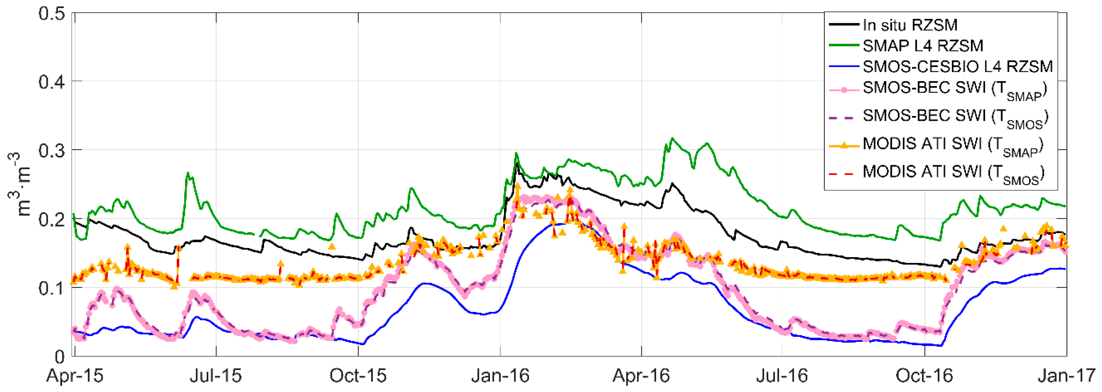
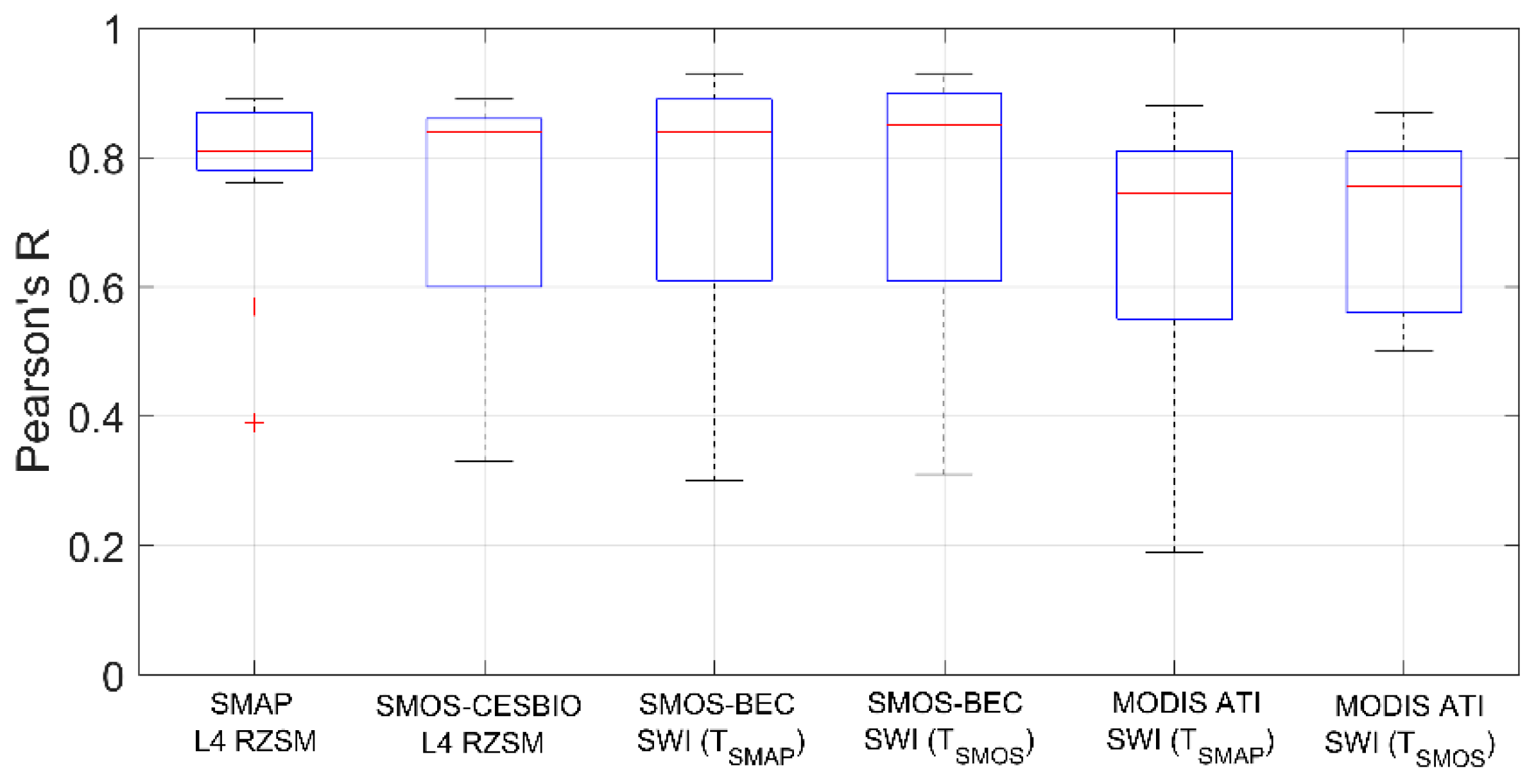
3.2. Temporal Analysis of Root Zone Soil Moisture Estimates

The pixel-average time series of the different RZSM estimates across REMEDHUS were compared against the station-average time series (Figure 2). At first glance, it is remarkable that all satellite datasets followed a temporal pattern similar to that of the in situ RZSM evolution, in agreement with the seasonality and climate of this region. It is highlighted that SMAP L4 RZSM and SMOS-BEC SWI had the best agreement with the dry-down and wetting-up events indicated by the in situ RZSM. To a lesser extent, this agreement also occurred for the MODIS ATI SWI, which fluctuated less. The SMOS-CESBIO L4 RZSM exhibited a certain time lag, especially during the rising periods, compared to the rest of the estimates. The reason could be the three-day window average of this product, which also smoothed the curve. While the SMOS SSM has proven more variable than the ground-based SSM itself [45,64], the SMOS RZSM showed more stability, which is consistent with the expected behavior of the deep soil moisture [43] that is typically more steady than the SSM.

In general, the SMAP L4 RZSM slightly overestimated the in situ RZSM but captured its overall variability well, with the bias almost constant. By contrast, the SMOS-CESBIO L4 RZSM underestimated the in situ RZSM, and the differences are higher during the dry season compared to the other estimates except for the SMOS-BEC SWI. This fact could be explained from the SMOS SSM underestimation previously detected in this area [45,64,65] and in other regions [66,67,68]. Both MODIS ATI SWIs also underestimated the in situ RZSM, although to a minor degree, while their agreement was better than with the other estimates, particularly during the dry season.

Regarding the impact of the T parameter, there were no differences in the use of T_SMAP and T_SMOS to derive the SWI, both with SMOS-BEC and MODIS ATI. This result could have occurred because they were very similar in the REMEDHUS area. Indeed, when computing the statistics of the T maps, the mean values of T_SMAP and T_SMOS were 14.5 and 17 days, the median values were 13 and 16.5 days, and the mode values were 13 and 16 days, respectively. It has been demonstrated that the T parameter is the response time of the autocorrelation function of soil moisture [37]. The T was affected by soil depth, soil hydraulic properties, and different physical processes such as evaporation and runoff. However, other processes such as transpiration or the soil hydraulic conductivity variation depending on soil moisture conditions were not considered in the SWI model [32,33]. Additionally, the potential dependence of T on soil texture was previously suggested [69]. Unfortunately, no significant relations were observed between T and soil properties (sand and clay fractions, bulk density, and organic matter content) [33]. The variability of the T parameter has previously been shown in several studies [32,33,37,38,39,40,42,43,69]. However, the SWI performed with similar good results in all cases. The robustness of SWI on the T parameter may rely on the recursive expression of the exponential filter, where the SSM has the highest influence and T only represents a timescale value.

The statistics obtained from the validation of the different RZSM estimates across REMEDHUS showed very similar correlation coefficients for all the estimates (by stations;

Table 2. Statistics obtained from comparison of the six RZSM estimates (by stations and area-average) with the in situ RZSM across REMEDHUS. N indicates the number of coincident data days.

RZSM Estimation			R	RMSD (m3/m3)	cRMSD (m3/m3)	bias (m3/m3)	N (%)
By stations	SMAP L4 RZSM		0.39 to 0.89	0.027 to 0.180	0.019 to 0.058	−0.036 to 0.177	86.3 to 99.7
	SMOS-CESBIO L4 RZSM		0.33 to 0.89	0.036 to 0.179	0.023 to 0.061	−0.174 to 0.006	86.5 to 99.8
	SMOS-BEC	SWI (TSMAP)	0.30 to 0.93	0.030 to 0.148	0.028 to 0.063	−0.143 to 0.033	78.3 to 91.1
		SWI (TSMOS)	0.31 to 0.93	0.027 to 0.148	0.024 to 0.061	−0.144 to 0.032	78.3 to 91.1
	MODIS ATI	SWI (TSMAP)	0.19 to 0.88	0.032 to 0.110	0.017 to 0.054	−0.098 to 0.057	44.9 to 53.4
		SWI (TSMOS)	0.18 to 0.87	0.031 to 0.110	0.017 to 0.053	−0.098 to 0.056	44.9 to 53.4
Area-average	SMAP L4 RZSM		0.86	0.044	0.020	0.040	99.7
	SMOS-CESBIO L4 RZSM		0.84	0.109	0.028	−0.105	99.8
	SMOS-BEC	SWI (TSMAP)	0.81	0.086	0.039	−0.077	92.7
		SWI (TSMOS)	0.82	0.086	0.037	−0.077	92.7
	MODIS ATI	SWI (TSMAP)	0.75	0.045	0.022	−0.038	68.1
		SWI (TSMOS)	0.77	0.044	0.021	−0.039	68.1

All values are significant (p-value < 0.05).

and Figure 3), although the correlations for MODIS ATI SWI (area-average) were slightly lower (R ~ 0.75 to 0.77). All correlations were significant at a 95 % confidence level. Similar correlation coefficient values were found in previous research when the SWI model was used. For instance, R ~ 0.45 to 0.88 was obtained when the SWI was applied to in situ SSM measurements of the Soil Climatic Analysis Network (SCAN) and compared to soil moisture measurements at 10–90 cm depth [34]. Likewise, R ~ 0.49 to 0.75 was obtained when the SWI was applied to the SMOS SSM and compared to the soil moisture of the 25–60 cm profile layer at the Oklahoma Mesonet and the Nebraska Automated Weather Data Network (AWDN) [42] and also compared to the soil moisture of the 0–50 cm depth of the same REMEDHUS network [43].

Regarding the differences from the in situ RZSM (Table 2), the values obtained for MODIS ATI SWI (RMSD ~ 0.031 to 0.110 m³/m³ and cRMSD ~ 0.017 to 0.054 m³/m³, by stations) were slightly lower than those for the other estimates (RMSD ~ 0.027 to 0.180 m³/m³ and cRMSD ~ 0.019 to 0.058 m³/m³) except for the SMAP L4 RZSM product, as expected from Figure 2. Both SMAP L4 RZSM and MODIS ATI SWI had the lowest differences (RMSD ~ 0.044 m³/m³ and cRMSD ~ 0.020–0.021 m³/m³, area-average), while SMOS-CESBIO L4 RZSM and SMOS-BEC SWI had the highest. These results suggested that MODIS ATI SWI could be a good estimator of RZSM at a spatial resolution of 1 km.

The bias (Table 2) of SMAP L4 RZSM exhibited positive values (by stations and area-average), indicating an overestimation of the in situ RZSM, whereas SMOS-CESBIO L4 RZSM, SMOS-BEC SWI and MODIS ATI SWI had dry biases in both cases, as observed in Figure 2. Different studies have shown that SMAP overestimates the SSM [2,59]. In this line, the SMAP L4 RZSM showed a slightly higher positive bias (0.063 m³/m³) during the validation of this product over the Little River. The irrigated crops and wetlands in the surroundings of this site, which are not considered in the SMAP model system, were first assumed as possible reasons for this wet bias, but REMEDHUS has no wetlands in its vicinity. Moreover, the wet bias over the Little River also appeared in the SMAP model-only simulations, suggesting that errors in the NASA catchment model parameters may be the main reason [30]. By contrast, the SMOS-derived RZSM estimates exhibited a dry bias (−0.15 to +0.05 m³/m³), with values similar to those previously observed [43].

In summary, it is remarkable that the results for the SMAP RZSM and SMOS SWI (R > 0.8 and cRMSD ~ 0.02 m³/m³) were better than those found in some works about SSM over the REMEDHUS network. For the SMOS L2 SSM product, the correlation was R ~ 0.78, and the errors were beyond cRMSD ~ 0.04 m³/m³ [45]. In the case of the SMAP L2 SSM product, the correlation was R ~ 0.58, and the errors were also close to cRMSD ~ 0.04 m³/m³ [2]. Moreover, the results obtained for SMAP RZSM in this research were near those found for the SSM product in REMEDHUS (R ~ 0.9) but for a longer period of validation [59].

A previous study suggested that the inherent differences between SMOS and in situ were larger than the errors produced by the SWI model [42]. This situation was also true here, where the RMSD and bias were smaller for the SWI-derived estimations than for the SMOS RZSM product itself. The impact of using T_SMOS or T_SMAP in the SWI model was negligible for both SMOS-BEC and MODIS ATI, and non-significant differences were found during the validation across REMEDHUS. It is highlighted that the coverage of MODIS ATI SWI was clearly lower than that of the other estimations by both stations and area-average, which evidenced the most important drawback of the MODIS ATI-derived RZSM owing the use of VIS/IR observations.

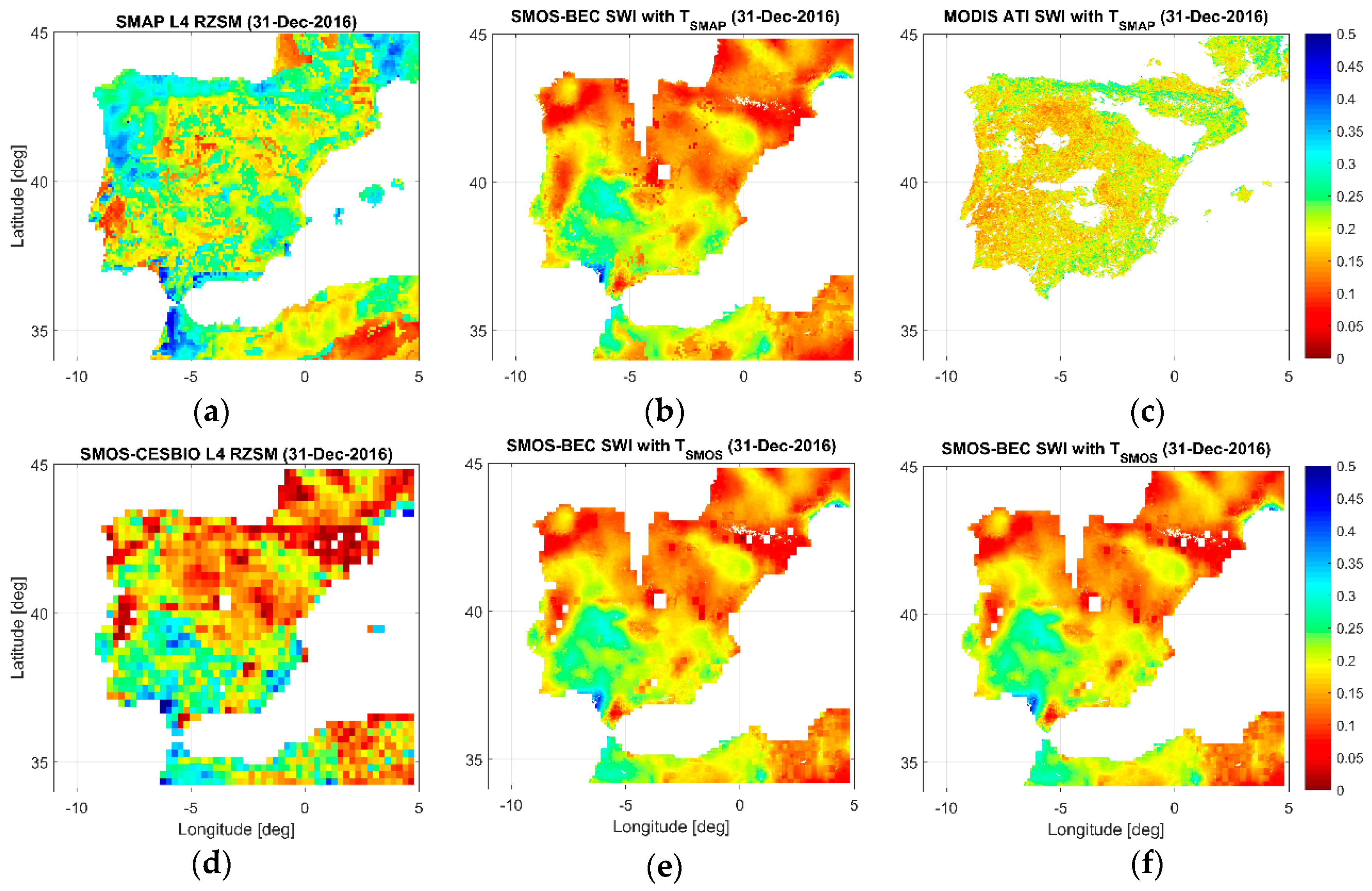
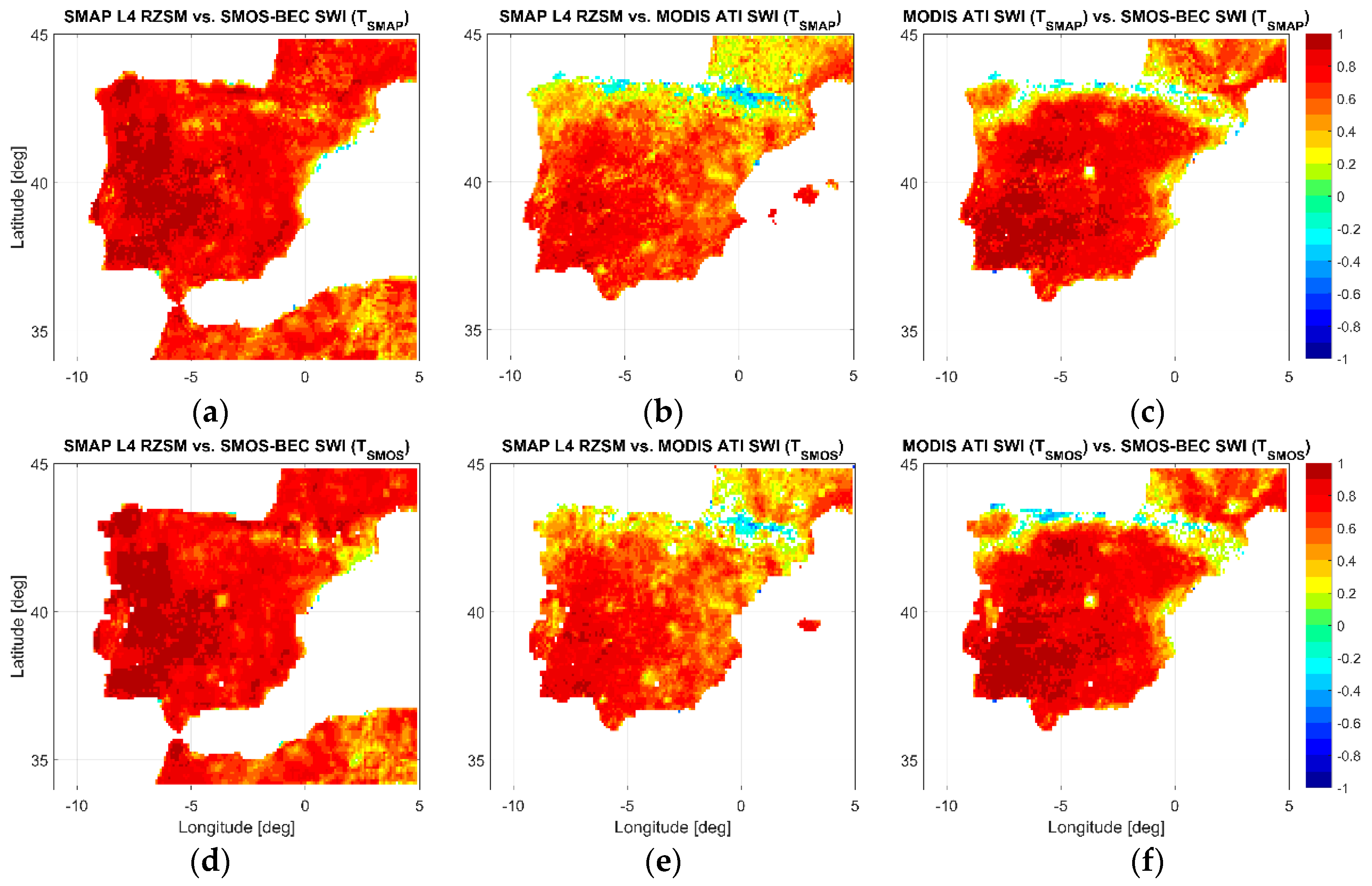
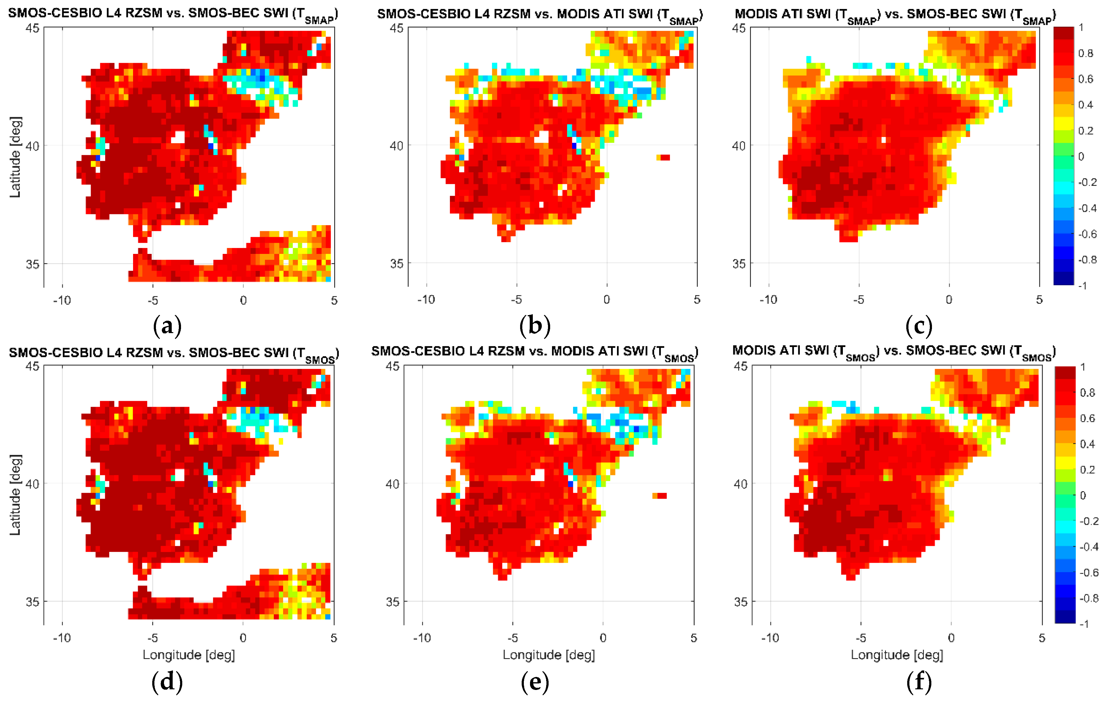
3.3. Spatial Analysis of Root Zone Soil Moisture Estimates

Six maps of RZSM over the Iberian Peninsula—one for each different RZSM estimate—are displayed during a summer and a winter day (9 July and 31 December 2016) in Figure 4 and Figure 5, respectively. No significant differences were observed between the SMOS-BEC and MODIS ATI SWI calculated with T_SMAP and T_SMOS, as it was seen in the REMEDHUS area (Table 2 and Figure 3). This result suggests that the T parameter could have a very small influence in the SWI model results.

On both dates, there was a high similarity between the SMOS-CESBIO L4 RZSM and the SMOS-BEC SWI maps because both estimations used data from the same radiometer and similar approaches were employed to obtain the RZSM. Note that the higher spatial resolution of the SMOS-BEC SWI maps allowed observing more details than that of the SMOS-CESBIO L4 RZSM maps. In general, although the SMOS-BEC SWI used both ascending and descending orbits to increase its coverage, the SMOS orbital path of a unique day usually does not cover the entire Iberian Peninsula and some data gaps are still present. Instead, the SMOS-CESBIO L4 RZSM covered the entire spatial domain since it was produced by a three day composite.

In general, the SMAP L4 RZSM product displayed wetter values than all the other estimates on both days, confirming the overestimation found in REMEDHUS. Additionally, the SMAP L4 RZSM maps clearly exhibited wetter values in the north than in the south, which was in accordance with the climatic patterns over the Iberian Peninsula. This effect was especially noticeable for the Pyrenees and the Cantabrian ranges in the north and the Galicia region and the northern part of Portugal in the northwestern Iberian Peninsula. The SMOS-CESBIO L4 RZSM maps also displayed this synoptic situation in the summer. In summer as well as winter, both SMAP and SMOS-CESBIO L4 RZSM were able to detect the Doñana National Park—the most important wetland in Spain—located at the Guadalquivir River mouth (southern Spain). This area was also captured by the SMOS-BEC SWI, whereas the MODIS ATI SWI did not show these distinctive features. There was no marked spatial contrast in RZSM for the MODIS ATI SWI maps throughout the Iberian Peninsula on both days except the high values in the north during the wet period. The MODIS ATI SWI can be masked not only by clouds but also by fog banks due to the use of optical observations. This effect was captured in the MODIS ATI SWI maps for the winter day where some river valleys in the center of the Iberian Peninsula did not have data.

The temporal correlation maps of the SMAP and SMOS-CESBIO L4 RZSM with both SMOS-BEC and MODIS ATI SWI aggregated to 9 km and 25 km are shown in Figure 6 and Figure 7, respectively. Only pixels with significant correlation (p-value < 0.05) are shown. It can be seen that microwave-based RZSM estimates (the SMAP L4 RZSM product at 9 km against SMOS-BEC SWI estimates) were highly correlated over most parts of the Iberian Peninsula (R ≥ 0.7), regardless of the T parameter used. Only some areas displayed low values of correlation (R ~ 0.2 to 0.3). These areas, such as the Pyrenees, had a low number of days with data because the abrupt topography decreased the number of soil moisture retrievals for these pixels. However, when comparing the SMAP L4 RZSM against the MODIS ATI SWI, the correlations over all the extreme north of the peninsula were low and even reached negative values, especially in regions with abundant and dense vegetation such as the Pyrenees and Cantrabrian ranges. The same patterns were obtained when comparing the MODIS ATI SWI against the SMOS-BEC SWI with both T parameter values. This result may be related to the distinctive vegetation of these regions because there are other mountainous areas in the Iberian Peninsula, but the north ranges are also the more densely forested ones.

In addition, a similar comparison was made with the SMOS-CESBIO L4 RZSM at 25 km, and the same patterns were distinguished irrespective of its lower spatial resolution compared to SMAP. The same patterns were found in the evapotranspiration and Fractional Vegetation Cover products from the Spinning Enhanced Visible and Infrared Imager (SEVIRI) sensor on board the Meteosat Second Generation (MSG) [70]. Then, the VIS/IR-based observations produced negative correlations in northern Spain. This result could be due to the MODIS variables involved in the ATI-derived soil moisture estimation (reflectance or LST). The reflectance was directly linked to the MODIS NDVI that was used to obtain the SMOS-BEC L4 SSM from its downscaling algorithm but not the MODIS LST. However, the observed correlation patterns were not seen in the correlations maps of the SMOS-BEC SWI with other passive RZSM estimates. Due to this fact, the reflectance was discarded as the cause of the negative correlations. Therefore, the reason for these correlation patterns may be the different characterization of the MODIS LST reflecting the north-south temperature gradient compared with the LSTs from the NASA catchment model and the ECMWF ERA-Interim model used in SMAP L4 RZSM and SMOS-BEC L4 SSM, respectively.

4. Conclusions

In recent years, the use of RZSM has become increasingly important in several hydrological and agricultural applications. In this research, six different RZSM estimates provided by three satellites—SMAP and SMOS operating at the microwave L-band and MODIS operating at the optical frequency range—were evaluated across the Iberian Peninsula from 31 March 2015 to 31 December 2016.

A preliminary analysis of the MODIS ATI-derived SSM estimation was carried out. It correctly reproduced the in situ SSM measurements with slightly lower correlations but a similar performance in terms of errors and bias than estimates obtained from the L-band. Because there were no remarkable differences between all possible alternatives to calculate the ATI-derived SSM, the approach that was easiest to implement, had the lowest computational cost, and with the best available spatial and temporal resolution was selected. This approach used the visible albedo reflectance, the combination of the Aqua/Terra LST, and the Soil Hydraulic Database to set the reference thresholds for soil moisture.

In the temporal analysis of the six RZSM estimates performed across the REMEDHUS area, all of them followed a similar evolution. The SMOS-CESBIO L4 RZSM product, the SMOS-BEC SWI, and MODIS ATI SWI showed underestimations with respect to the in situ measurements, while the SMAP L4 RZSM product showed overestimation. The different alternatives for T parameters used in the SWI model did not seem to impact the results.

In the spatial analysis performed across the Iberian Peninsula, a high level of similarity was observed between the SMOS-based estimations, with clearly higher spatial detail for the SMOS-BEC SWI than for the other estimates. The most distinctive spatial variability between wet and dry regions was displayed by the SMAP L4 RZSM, whereas the MODIS ATI SWI had the lowest spatial variability.

Regarding the correlation spatial patterns, the RZSM estimates from the microwave sensors were highly correlated across the Iberian Peninsula except in areas with low amounts of data. The comparison between microwave and optical observations showed low or negative correlation values all over the extreme north of the peninsula, coinciding with the location of higher mountains and more densely forested areas.

Although two different spectral regions were used (microwave or optical frequencies), all six different RZSM estimates reproduced the temporal patterns of the in situ RZSM well and could be considered as good RZSM estimators. The SWI model, which required only SSM and the T parameter as inputs, worked as well as more complex land surface or hydrological models for estimating RZSM, as in the cases of the SMOS and SMAP L4 RZSM products. The good results based on the MODIS ATI must be highlighted, despite its lesser temporal coverage, given MODIS is not a satellite mission specifically devoted to soil moisture retrieval.

The use of remote sensing as an alternative to ground-based measurements for RZSM monitoring offers a new opportunity for hydrological studies and agricultural applications at the global scale, improving their spatial coverage and temporal resolution.

References

1. Kerr, Y.H.; Al-Yaari, A.; Rodríguez-Fernández, N.; Parrens, M.; Molero, B.; Leroux, D.; Bircher, S.; Mahmoodi, A.; Mialon, A.; Richaume, P.; et al. Overview of SMOS performance in terms of global soil moisture monitoring after six years in operation. Remote Sens. Environ. 2016, 180, 40–63. [Google Scholar] [CrossRef]
2. Chan, S.K.; Bindlish, R.; O’Neill, P.E.; Njoku, E.; Jackson, T.J.; Colliander, A.; Chen, F.; Burgin, M.; Dunbar, S.; Piepmeier, J.; et al. Assessment of the SMAP passive sol moisture product. IEEE Trans. Geosci. Remote Sens. 2016, 54, 4994–5007. [Google Scholar] [CrossRef]
3. Piles, M.; Sánchez, N.; Vall-llossera, M.; Camps, A.; Martínez-Fernández, J.; Martínez, J.; González-Gambau, V. A downscaling approach for SMOS land observations: Evaluation of high-resolution soil moisture maps over the Iberian Peninsula. IEEE J. Sel. Top. Appl. Earth Observ. Remote Sens. 2014, 7, 3845–3857. [Google Scholar] [CrossRef]
4. Merlin, O.; Malbéteau, Y.; Notfi, Y.; Bacon, S.; Khabba, S.E.R.; Jarlan, L. Performance metrics for soil moisture downscaling methods: Application to DISPATCH data in central Morocco. Remote Sens. 2015, 7, 3783–3807. [Google Scholar] [CrossRef]
5. Pablos, M.; Piles, M.; Sánchez, N.; Vall-llossera, M.; Martínez-Fernández, J.; Camps, A. Impact of day/night time land surface temperature in soil moisture disaggregation algorithms. Eur. J. Remote Sens. 2016, 49, 899–916. [Google Scholar] [CrossRef] [Green Version]
6. Piles, M.; Petropoulos, G.P.; Sánchez, N.; González-Zamora, A.; Ireland, G. Towards improved spatio-temporal resolution soil moisture retrievals from the synergy of SMOS and MSG SEVIRI spaceborne observations. Remote Sens. Environ. 2016, 180, 403–417. [Google Scholar] [CrossRef] [Green Version]
7. Das, N.N.; Entekhabi, D.; Dunbar, R.S.; Njoku, E.G.; Yueh, S.H. Uncertainty estimates in the SMAP combined active & passive downscaled brightness temperature. IEEE Trans. Geosci. Remote Sens. 2016, 54, 640–650. [Google Scholar] [CrossRef]
8. Petropoulos, G.P.; Ireland, G.; Barrett, B. Surface soil moisture retrievals from remote sensing: Current status, products & future trends. Phy. Chem. Earth Parts A/B/C 2015, 83–84, 36–56. [Google Scholar] [CrossRef]
9. Price, J.C. Thermal inertia mapping: A new view of the Earth. J. Geophys. Res. 1977, 82, 2582–2590. [Google Scholar] [CrossRef]
10. Short, N.M.; Stuart, L.M. The Heat Capacity Mapping Mission (HCMM) Anthology; Scientific and technical information banch; National Aeronautics and Space Administration (NASA): Washington, DC, USA, 1983; p. 264. [Google Scholar]
11. Sobrino, J.A.; El Kharraz, M.H. Combining afternoon and morning NOAA satellites for thermal inertia estimation: 1. Algorithm and its testing with Hydrologic Atmospheric Pilot Experiment-Sahel data. J. Geophys. Res. Atmos. 1999, 104, 9445–9453. [Google Scholar] [CrossRef] [Green Version]
12. Verstraeten, W.W.; Veroustraete, F.; van der Sande, C.J.; Grootaers, I.; Feyen, J. Soil moisture retrieval using thermal inertia, determined with visible and thermal spaceborne data, validated for European forests. Remote Sens. Environ. 2006, 101, 299–314. [Google Scholar] [CrossRef]
13. Van doninck, J.; Peters, J.; De Baets, B.; De Clercq, E.M.; Ducheyne, E.; Verhoest, N.E.C. The potential of multitemporal Aqua and Terra MODIS apparent thermal inertia as a soil moisture indicator. Int. J. Appl. Earth Observ. Geoinf. 2011, 13, 934–941. [Google Scholar] [CrossRef]
14. Vereecken, H.; Huisman, J.A.; Bogena, H.; Vanderborght, J.; Vrugt, J.A.; Hopmans, J.W. On the value of soil moisture measurements in vadose zone hydrology: A review. Water Resour. Res. 2008, 44, 1–21. [Google Scholar] [CrossRef]
15. Mohanty, B.P.; Cosh, M.H.; Lakshmi, V.; Montzka, C. Soil moisture remote sensing: State-of-the-science. Vadose Zone J. 2017, 16, 1–9. [Google Scholar] [CrossRef]
16. Dorigo, W.A.; Wagner, W.; Hohensinn, R.; Hahn, S.; Paulik, C.; Xaver, A.; Gruber, A.; Drusch, M.; Mecklenburg, S.; van Oevelen, P.; et al. The International Soil Moisture Network: A data hosting facility for global in situ soil moisture measurements. Hydrol. Earth Syst. Sci. 2011, 15, 1675–1698. [Google Scholar] [CrossRef]
17. Zreda, M.; Shuttleworth, W.J.; Zeng, X.; Zweck, C.; Desilets, D.; Franz, T.; Rosolem, R. COSMOS: The COsmic-ray Soil Moisture Observing System. Hydrol. Earth Syst. Sci. 2012, 16, 4079–4099. [Google Scholar] [CrossRef] [Green Version]
18. Kędzior, M.; Zawadzki, J. Comparative study of soil moisture estimations from SMOS satellite mission, GLDAS database, and cosmic-ray neutrons measurements at COSMOS station in Eastern Poland. Geoderma 2016, 283, 21–31. [Google Scholar] [CrossRef]
19. Zreda, M.; Desilets, D.; Ferré, T.P.A.; Scott, R.L. Measuring soil moisture content non-invasively at intermediate spatial scale using cosmic-ray neutrons. Geophys. Res. Lett. 2008, 35, 1–5. [Google Scholar] [CrossRef]
20. Liu, X.; Chen, J.; Cui, X.; Liu, Q.; Cao, X.; Chen, X. Measurement of soil water content using ground-penetrating radar: A review of current methods. Int. J. Dig. Earth 2017, 1–24. [Google Scholar] [CrossRef]
21. Haddeland, I.; Clark, D.B.; Franssen, W.; Ludwig, F.; Voß, F.; Arnell, N.W.; Bertrand, N.; Best, M.; Folwell, S.; Gerten, D.; et al. Multimodel estimate of the global terrestrial water balance: Setup and first results. J. Hydrometeorol. 2011, 12, 869–884. [Google Scholar] [CrossRef]
22. Muñoz-Sabater, J.; Jarlan, L.; Calvet, J.C.; Bouyssel, F.; De Rosnay, P. From near-surface to root-zone soil moisture using different assimilation techniques. J. Hydrometeorol. 2007, 8, 194–206. [Google Scholar] [CrossRef]
23. Das, N.N.; Mohanty, B.P.; Njoku, E.G. Profile soil moisture across spatial scales under different hydroclimatic conditions. Soil Sci. 2010, 175, 315–319. [Google Scholar] [CrossRef]
24. Dumedah, G.; Walker, J.P. Evaluation of model parameter convergence when using data assimilation for soil moisture estimation. J. Hydrometeorol. 2014, 15, 359–375. [Google Scholar] [CrossRef]
25. Calvet, J.-C.; Noilhan, J. From near-surface to root-zone soil moisture using year-round data. J. Hydrometeorol. 2000, 1, 393–411. [Google Scholar] [CrossRef]
26. Montaldo, N.; Albertson, J.D.; Mancini, M.; Kiely, G. Robust simulation of root zone soil moisture with assimilation of surface soil moisture data. Water Resour. Res. 2001, 37, 2889–2900. [Google Scholar] [CrossRef] [Green Version]
27. Reichle, R.H.; Koster, R.D.; Liu, P.; Mahanama, S.P.P.; Njoku, E.G.; Owe, M. Comparison and assimilation of global soil moisture retrievals from the Advanced Microwave Scanning Radiometer for the Earth Observing System (AMSR-E) and the Scanning Multichannel Microwave Radiometer (SMMR). J. Geophys. Res. Atmos. 2007, 112, 1–14. [Google Scholar] [CrossRef]
28. Draper, C.; Mahfouf, J.-F.; Calvet, J.-C.; Martin, E.; Wagner, W. Assimilation of ASCAT near-surface soil moisture into the SIM hydrological model over France. Hydrol. Earth Syst. Sci. 2011, 15, 3829–3841. [Google Scholar] [CrossRef] [Green Version]
29. Dumedah, G.; Walker, J.P.; Merlin, O. Root-zone soil moisture estimation from assimilation of downscaled Soil Moisture and Ocean Salinity data. Adv. Water Resour. 2015, 84, 14–22. [Google Scholar] [CrossRef]
30. Reichle, R.H.; De Lannoy, G.J.M.; Liu, Q.; Ardizzone, J.V.; Colliander, A.; Conaty, A.; Crow, W.; Jackson, T.J.; Jones, L.A.; Kimball, J.S.; et al. Assessment of the SMAP level-4 surface and root-zone soil moisture product using in situ measurements. J. Hydrometeorol. 2017, 18, 2621–2645. [Google Scholar] [CrossRef]
31. Al Bitar, A.; Kerr, Y.H.; Merlin, O.; Cabot, F.; Wigneron, J.P. Global Drought Index from SMOS Soil Moisture. In Proceedings of the IEEE International Geoscience and Remote Sensing Symposium (IGARSS), Melbourne, Australia, 21–26 July 2013. [Google Scholar]
32. Wagner, W.; Lemoine, G.; Rott, H. A method for estimating soil moisture from ERS scatterometer and soil data. Remote Sens. Environ. 1999, 70, 191–207. [Google Scholar] [CrossRef]
33. Albergel, C.; Rüdiger, C.; Pellarin, T.; Calvet, J.-C.; Fritz, N.; Froissard, F.; Suquia, D.; Petitpa, A.; Piguet, B.; Martin, E. From near-surface to root-zone soil moisture using an exponential filter: An assessment of the method based on in-situ observations and model simulations. Hydrol. Earth Syst. Sci. Discuss. 2008, 12, 1323–1337. [Google Scholar] [CrossRef]
34. Manfreda, S.; Brocca, L.; Moramarco, T.; Melone, F.; Sheffield, J. A physically based approach for the estimation of root-zone soil moisture from surface measurements. Hydrol. Earth Syst. Sci. 2014, 18, 1199–1212. [Google Scholar] [CrossRef] [Green Version]
35. Qiu, J.; Crow, W.T.; Nearing, G.S.; Mo, X.; Liu, S. The impact of vertical measurement depth on the information content of soil moisture times series data. Geophys. Res. Lett. 2014, 41, 4997–5004. [Google Scholar] [CrossRef] [Green Version]
36. Peterson, A.M.; Helgason, W.D.; Ireson, A.M. Estimating field-scale root zone soil moisture using the cosmic-ray neutron probe. Hydrol. Earth Syst. Sci. 2016, 20, 1373–1385. [Google Scholar] [CrossRef] [Green Version]
37. Ceballos, A.; Scipal, K.; Wagner, W.; Martínez-Fernández, J. Validation of ERS scatterometer-derived soil moisture data in the central part of the Duero Basin, Spain. Hydrol. Process. 2005, 19, 1549–1566. [Google Scholar] [CrossRef]
38. Brocca, L.; Melone, F.; Moramarco, T.; Wagner, W.; Hasenauer, S. ASCAT soil wetness index validation through in situ and modeled soil moisture data in central Italy. Remote Sens. Environ. 2010, 114, 2745–2755. [Google Scholar] [CrossRef]
39. Brocca, L.; Hasenauer, S.; Lacava, T.; Melone, F.; Moramarco, T.; Wagner, W.; Dorigo, W.; Matgen, P.; Martínez-Fernández, J.; Llorens, P.; et al. Soil moisture estimation through ASCAT and AMSR-E sensors: An intercomparison and validation study across Europe. Remote Sens. Environ. 2011, 115, 3390–3408. [Google Scholar] [CrossRef]
40. Paulik, C.; Dorigo, W.; Wagner, W.; Kidd, R. Validation of the ASCAT Soil Water Index using in situ data from the International Soil Moisture Network. Int. J. Appl. Earth Observ. Geoinf. 2014, 30, 1–8. [Google Scholar] [CrossRef]
41. Tobin, K.J.; Torres, R.; Crow, W.T.; Bennett, M.E. Multi-decadal analysis of root-zone soil moisture applying the exponential filter across CONUS. Hydrol. Earth Syst. Sci. 2017, 21, 4403–4417. [Google Scholar] [CrossRef] [Green Version]
42. Ford, T.W.; Harris, E.; Quiring, S.M. Estimating root zone soil moisture using near-surface observations from SMOS. Hydrol. Earth Syst. Sci. 2014, 18, 139–154. [Google Scholar] [CrossRef] [Green Version]
43. González-Zamora, A.; Sánchez, N.; Martínez-Fernández, J.; Wagner, W. Root-zone plant available water estimation using the SMOS-derived soil water index. Adv. Water Resour. 2016, 96, 339–353. [Google Scholar] [CrossRef]
44. González-Zamora, A.; Martínez-Fernández, J.; Sánchez, N.; Pablos, M. Estimación de la humedad en la zona radicular a partir de observaciones remotes de humedad superficial de larga duración. In Las XIII de Jornadas de Investigación de la Zona No Saturada; Moret-Fernández, D., López, M.V., Eds.; Consejo Superior de Investigaciones Científicas (CSIC): Zaragoza, Spain, 2017; Volume XIII, pp. 493–504. [Google Scholar]
45. González-Zamora, A.; Sánchez, N.; Martínez-Fernández, J.; Gumuzzio, A.; Piles, M.; Olmedo, E. Long-term SMOS soil moisture products: A comprehensive evaluation across scales and methods in the Duero Basin (Spain). Phys. Chem. Earth Parts A/B/C 2015, 83–84, 123–136. [Google Scholar] [CrossRef]
46. Reichle, R.H.; De Lannoy, G.; Koster, R.D.; Crow, W.T.; Kimball, J.S. SMAP L4 9 km EASE-Grid Surface and Root Zone Soil Moisture Geophysical Data, Version 3; National Snow and Ice Data Center Distributed Active Archive Center (NSIDC DAAC): Boulder, CO, USA, 2017. [Google Scholar]
47. Reichle, R.H.; Koster, R.D.; De Lannoy, G.J.M.; Crow, W.T.; Kimball, J. Algorithm Theoretical Basis Document Level 4 Surface and Root Zone Soil Moisture (L4_SM) Data Product; National Aerounautics and Space Administration (NASA): Greenbelt, MD, USA, 2014; pp. 1–65.
48. Kerr, Y.H.; Jacquette, E.; Al Bitar, A.; Cabot, F.; Mialon, A.; Richaume, P.; Quesney, A.; Berthon, L. CATDS SMOS L3 Soil Moisture Retrieval Processor Algorithm Theoretical Baseline Document (ATBD); Centre Aval de Traitement des Données SMOS (CATDS): Toulouse, France, 2013. [Google Scholar]
49. Kerr, Y.H.; Waldteufel, P.; Richaume, P.; Wigneron, J.P.; Ferrazzoli, P.; Mahmoodi, A.; Bitar, A.A.; Cabot, F.; Gruhier, C.; Juglea, S.E.; et al. The SMOS soil moisture retrieval algorithm. IEEE Trans. Geosci. Remote Sens. 2012, 50, 1384–1403. [Google Scholar] [CrossRef]
50. Al Bitar, A.; Mialon, A.; Kerr, Y.H.; Cabot, F.; Richaume, P.; Jacquette, E.; Quesney, A.; Mahmoodi, A.; Tarot, S.; Parrens, M.; et al. The global SMOS Level 3 daily soil moisture and brightness temperature maps. Earth Syst. Sci. Data 2017, 9, 293–315. [Google Scholar] [CrossRef] [Green Version]
51. Portal, G.; Vall-llossera, M.; Piles, M.; Camps, A.; Chaparro, D.; Pablos, M.; Rossato, L. A spatially consistent downscaling approach for SMOS using an adaptive moving window. IEEE J. Sel. Top. Appl. Earth Observ. Remote Sens. 2018, in press. [Google Scholar] [CrossRef]
52. Vermote, E.F.; Vermeulen, A. Atmospheric Correction Algorithm: Spectral Reflectances (MOD09) Version 4.0; National Aeronautics and Space Administration (NASA): Washington, DC, USA; Department of Geography, University of Maryland: College Park, MD, USA, 1999. [Google Scholar]
53. Wan, Z. MODIS Land-Surface Temperature Algorithm Theoretical Basis Document (LST ATBD) Version 3.3; National Aeronautics and Space Administration (NASA): Washington, DC, USA; Institute for Computational Earth System Science, University of California: Santa Barbara, CA, USA, 1999.
54. Liang, S. Narrowband to broadband conversions of land surface albedo I: Algorithms. Remote Sens. Environ. 2001, 76, 213–238. [Google Scholar] [CrossRef]
55. Pablos, M.; Martínez-Fernández, J.; Piles, M.; Sánchez, N.; Vall-llossera, M.; Camps, A. Multi-temporal evaluation of soil moisture and land surface temperature dynamics using in situ and satellite observations. Remote Sens. 2016, 8, 587. [Google Scholar] [CrossRef]
56. Toté, C.; Patricio, D.; Boogaard, H.; van der Wijngaart, R.; Tarnavsky, E.; Funk, C. Evaluation of satellite rainfall estimates for frought and food monitoring in Mozambique. Remote Sens. 2015, 7, 1758–1776. [Google Scholar] [CrossRef]
57. Chang, T.Y.; Wang, Y.C.; Feng, C.C.; Ziegler, A.D.; Giambelluca, T.W.; Liou, Y.A. Estimation of root zone soil moisture using apparent thermal inertia with MODIS imagery over a tropical catchment in northern Thailand. IEEE J. Sel. Top. Appl. Earth Observ. Remote Sens. 2012, 5, 752–761. [Google Scholar] [CrossRef]
58. Dorigo, W.; Wagner, W.; Albergel, C.; Albrecht, F.; Balsamo, G.; Brocca, L.; Chung, D.; Ertl, M.; Forkel, M.; Gruber, A.; et al. ESA CCI soil moisture for improved Earth system understanding: State-of-the art and future directions. Remote Sens. Environ. 2017, 203, 185–215. [Google Scholar] [CrossRef]
59. Colliander, A.; Jackson, T.J.; Bindlish, R.; Chan, S.; Das, N.; Kim, S.B.; Cosh, M.H.; Dunbar, R.S.; Dang, L.; Pashaian, L.; et al. Validation of SMAP surface soil moisture products with core validation sites. Remote Sens. Environ. 2017, 191, 215–231. [Google Scholar] [CrossRef]
60. González-Zamora, Á.; Sánchez, N.; Pablos, M.; Martínez-Fernández, J. CCI soil moisture assessment with SMOS soil moisture and in situ data under different environmental conditions and spatial scales in Spain. Remote Sens. Environ. 2018. [Google Scholar] [CrossRef]
61. Wang, K.; Liang, S.; Schaaf, C.L.; Strahler, A.H. Evaluation of Moderate Resolution Imaging Spectroradiometer land surface visible and shortwave albedo products at FLUXNET sites. J. Geophys. Res. Atmos. 2010, 115, 1–8. [Google Scholar] [CrossRef]
62. Qin, J.; Yang, K.; Lu, N.; Chen, Y.; Zhao, L.; Han, M. Spatial upscaling of in-situ soil moisture measurements based on MODIS-derived apparent thermal inertia. Remote Sens. Environ. 2013, 138, 1–9. [Google Scholar] [CrossRef]
63. Gao, S.; Zhu, Z.; Weng, H.; Zhang, J. Upscaling of sparse in situ soil moisture observations by integrating auxiliary information from remote sensing. Int. J. Remote Sens. 2017, 38, 4782–4803. [Google Scholar] [CrossRef]
64. Sánchez, N.; Martinez-Fernández, J.; Scaini, A.; Pérez-Gutiérrez, C. Validation of the SMOS L2 soil moisture data in the REMEDHUS network (Spain). IEEE Trans. Geosci. Remote Sens. 2012, 50, 1602–1611. [Google Scholar] [CrossRef]
65. Gumuzzio, A.; Brocca, L.; Sánchez, N.; González-Zamora, A.; Martínez-Fernández, J. Comparison of SMOS, modelled and in situ long-term soil moisture series in the northwest of Spain. Hydrol. Sci. J. 2016, 61, 2610–2625. [Google Scholar] [CrossRef]
66. Dall’Amico, J.T.; Schlenz, F.; Loew, A.; Mauser, W. First results of SMOS soil moisture validation in the Upper Danube Catchment. IEEE Trans. Geosci. Remote Sens. 2012, 50, 1507–1516. [Google Scholar] [CrossRef]
67. Dente, L.; Su, Z.; Wen, J. Validation of SMOS soil moisture products over the Maqu and Twente regions. Sensors 2012, 12, 9965–9986. [Google Scholar] [CrossRef] [PubMed]
68. Djamai, N.; Magagi, R.; Goïta, K.; Hosseini, M.; Cosh, M.H.; Berg, A.; Toth, B. Evaluation of SMOS soil moisture products over the CanEx-SM10 area. J. Hydrol. 2015, 520, 254–267. [Google Scholar] [CrossRef]
69. de Lange, R.; Beck, R.; van de Giesen, N.; Friesen, J.; de Wit, A.; Wagner, W. Scatterometer-Derived Soil Moisture Calibrated for Soil Texture with a One-Dimensional Water-Flow Model. IEEE Trans. Geosci. Remote Sens. 2008, 46, 4041–4049. [Google Scholar] [CrossRef]
70. Petropoulos, G.P.; Ireland, G.; Lamine, S.; Griffiths, H.M.; Ghilain, N.; Anagnostopoulos, V.; North, M.R.; Srivastava, P.K.; Georgopoulou, H. Operational evapotranspiration estimates from SEVIRI in support of sustainable water management. Int. J. Appl. Earth Observ. Geoinf. 2016, 49, 175–187. [Google Scholar] [CrossRef]
Figure 1. Flowchart showing all data and methodology applied to obtain the RZSM estimates.
Remotesensing 10 00981 g001
Figure 2. Average time series of the different RZSM estimates across REMEDHUS.
Remotesensing 10 00981 g002
Figure 3. Pearson’s correlation coefficients (R) between the in situ RZSM and the six RZSM estimates across REMEDHUS (by stations).
Remotesensing 10 00981 g003
Figure 4. RZSM maps corresponding to a summer day (9 July 2016): (a) SMAP L4 RZSM; (b) SMOS-BEC SWI (TSMAP); (c) MODIS ATI SWI (TSMAP); (d) SMOS-CESBIO L4 RZSM; (e) SMOS-BEC SWI (TSMOS); and (f) MODIS ATI SWI (TSMOS).
Remotesensing 10 00981 g004
Figure 5. RZSM maps corresponding to a winter day (31 December 2016): (a) SMAP L4 RZSM; (b) SMOS-BEC SWI (TSMAP); (c) MODIS ATI SWI (TSMAP); (d) SMOS-CESBIO L4 RZSM; (e) SMOS-BEC SWI (TSMOS); and (f) MODIS ATI SWI (TSMOS).
Remotesensing 10 00981 g005
Figure 6. Temporal correlation maps at 9 km between: (a) SMAP L4 RZSM and SMOS-BEC SWI (TSMAP); (b) SMAP L4 RZSM and MODIS ATI SWI (TSMAP); (c) MODIS ATI SWI (TSMAP) and SMOS-BEC (TSMAP); (d) SMAP L4 RZSM and SMOS-BEC SWI (TSMOS); (e) SMAP L4 RZSM and MODIS ATI SWI (TSMOS); and (f) MODIS ATI SWI (TSMOS) and SMOS-BEC (TSMOS).
Remotesensing 10 00981 g006
Figure 7. Temporal correlation maps at 25 km between: (a) SMOS-CESBIO L4 RZSM and SMOS-BEC SWI (TSMAP); (b) SMOS-CESBIO L4 RZSM and MODIS ATI SWI (TSMAP); (c) MODIS ATI SWI (TSMAP) and SMOS-BEC (TSMAP); (d) SMOS-CESBIO L4 RZSM and SMOS-BEC SWI (TSMOS); (e) SMOS-CESBIO L4 RZSM and MODIS ATI SWI (TSMOS); and (f) MODIS ATI SWI (TSMOS) and SMOS-BEC (TSMOS).
Remotesensing 10 00981 g007