1. Introduction
Image matching aims to find feature correspondences among two or more images, and it is a crucial step in many remote sensing applications such as image registration, change detection, 3D scene reconstruction, and aerial triangulation. Among all the matching methods, feature-based matching methods receive the most attention. These methods can be summarized in three steps: (1) feature detection; (2) feature description; and (3) descriptor matching.
In feature detection, salient features such as corners, blobs, lines, and regions are extracted from images. The commonly used feature detection methods are Harris corner detector [
1], features from accelerated segment test (FAST) [
2], differences of Gaussian (DoG) features [
3], binary robust invariant scalable (BRISK) features [
4], oriented FAST and rotation BRIEF (ORB) [
5], Canny [
6], and maximally stable external regions (MSER) [
7]. Among these image features, Harris, FAST, and DoG are point features which are invariant to image rotation. In particular, DoG is invariant to scale and linear illumination changes. Canny and MSER are line and region feature, respectively.
In the feature description, every image feature is assigned to a unique signature to distinguish itself from others so that the similar features will have close descriptors, while different features will characterize far different descriptors. State-of-the-art feature descriptors include scale-invariant feature transform (SIFT) [
3], speeded-up robust features (SURF) [
8], principle component analysis SIFT (PCA-SIFT) [
9], gradient location and orientation histogram (GLOH) [
10], local self-similarity (LSS) [
11], distinctive order-based self-similarity (DOBSS) [
12], local intensity order pattern (LIOP) [
13], and a multi-support region order-based gradient histogram (MROGH) [
14]. For line features, the mean-standard deviation line descriptor (MSLD) [
15] and line intersection context feature (LICF) [
16] have good performances. For region features, Forssén and Lowe [
17] gave their solution based on SIFT descriptor.
In the descriptor matching, the similarities between one feature and its candidates are evaluated by the distances of description vectors. The commonly used distance metrics for descriptor matching are Euclidean distance, Hamming distance, Mahalanobis distance, and a normalized correlation coefficient. To determine the final correspondences, sometimes a threshold, such as the nearest neighbor distance ratio (NNDR) [
3], is applied in descriptor matching.
Though many researchers have made massive improvements in the aforementioned matching steps in trying to obtain stable and practical matching results, matching multi-sensor remote sensing images is still a challenging task. The matching difficulties are the results of two issues. First, images of the same scene from different sensors often present different radiometric characteristics which are known as non-linear intensity differences [
12,
18]. These intensity differences can be exampled by
Figure 1a, showing a pair of images acquired by Ziyuan-3 (ZY-3) and Gaofen-1 (GF-1) sensors. Due to non-linear intensity differences caused by different sensors and illumination, the distance between local descriptors of two conjugated feature points are not close enough, and thus lead to false matches. Second, images from different sensors are often shot at different moments which gives rise to considerable textural changes. As shown in
Figure 1b, this image pair was captured by ZY-3 and Gaofen-2 (GF-2) sensors. The shot time spans over three years, and the rapid changes of the modern city resulted in abundant textural changes among images. Textural changes will bring down the repetitive rate of image features and lead to fewer correct matches. Both of these aspects reduce the matching recall [
10] and thus lead to unsatisfying matching results.
As the most representative method of feature-based matching, SIFT-based methods have been studied extensively. Its upgraded versions are successfully applied in matching multi-sensor remote sensing images. Yi et al. [
19] proposed gradient orientation modification SIFT (GOM-SIFT) which modified the gradient orientation of SIFT and gave restrictions on scale changes to improve the matching precision. The simple strategy was also used by Mehmet et al. [
20]; they proposed an orientation-restricted SIFT (OR-SIFT) descriptor which only had half the length of GOM-SIFT. When non-linear intensity differences and considerable textural changes are present between images, simply reversing the gradient orientation of image features cannot increase the number of correct matches. Hasan et al. [
21] took advantage of neighborhood information from SIFT’s key points. The experimental results showed that this method could generate more correct matches because the geometric structures between images were relatively static. Saleem and Sablatnig [
22] used normalized gradients SIFT (NG-SIFT) for matching multispectral images; their results showed that the proposed method achieved a better matching performance against non-linear intensity changes between multispectral images.
Considering the self-similarity of an image patch, local self-similarity (LSS) captures the internal geometric layouts of feature points. LSS is another theory which has been successfully applied for the registration of thermal and visible videos, and it has handled complex intensity variations. Shechtman [
11] first proposed the LSS descriptor and used it as an image-based and video-based similarity measure. Kim et al. [
23] improved LSS based on the observation that a self-similarity existing within images was less sensitive to modality variations. They proposed a dense adaptive self-correlation (DASC) descriptor for multi-modal and multi-spectral correspondences. In an earlier study, Kim et al. [
24] extended the standard LSS descriptor into the frequency domain and proposed the LSS frequency (LSSF) descriptor in matching multispectral and RGB-NIR image pairs. Their experimental results showed LSSF was invariant to image rotation, and it outperformed other state-of-the-art descriptors.
Despite the attractive illumination-invariance property, both standard LSS and extended LSS have drawbacks in remote sensing image matching because of their relatively low descriptor discriminability. To conquer this shortcoming, Ye and San [
18] used GOM-SIFT in the coarse registration process, and then utilized LSS descriptor for finding feature correspondences in the fine registration process. Their proposed method alleviated the low distinctiveness effect of LSS descriptors and achieved satisfied matching results in multispectral remote sensing image pairs. Sedaghat and Ebadi [
12] combined the merits of LSS and the intensity order pooling scheme, and proposed DOBSS for matching multi-senor remote sensing images. Similar to Ye and San’s matching strategy [
18], Liu et al. [
25] proposed a multi-stage matching approach for multi-source optical satellite imagery matching. They firstly estimated homographic transformation between source and target image by initial matching, and then used probability relaxation to expand matching. Though the matching scheme presented in [
25] obtained satisfied matching results in satellite images, it has the same defect as in [
18] that if the initial matching fails, the whole matching process will end up with a failure.
Most feature-based matching methods boil down to finding the closest descriptor in distance while seldom considering the topological structures between image features. In multi-sensor image pairs, non-linear intensity differences lead to dissimilarities of conjugate features in radiometry, and changed textures caused by different shooting moments have no feature correspondences in essence. Descriptor-based matching recall, which is a very crucial factor for a robust matching method, only depends on the radiometric similarity of feature pairs. On the contrary, although captured by different sensors or shot in different moments, the structures among images remain relatively static [
22], and they are invariant to intensity changes. Therefore, structural information can be utilized to obtain robust and reliable matching results. Based on this fact, many researchers cast the feature correspondence problem as the graph matching problem (e.g., [
26,
27,
28,
29]). The affinity tensor between graphs, as the core of graph matching [
26], paves the way for multi-sensor remote sensing image matching, since radiometric and geometric information of image features can be easily encoded in a tensor. Duchenne et al. [
28] used geometric constraints in feature matching and gained favorable matching results. Wang et al. [
30] proposed a new matching method based on a multi-tensor which merged multi-granularity geometric affinities. The experimental results showed that their method was more robust than the method proposed in [
28]. Chen et al. [
31] observed that outliers were inevitable in matching, so they proposed a weighted affinity tensor for poor textural image matching and gained better experimental results compared to feature-based matching algorithms.
To address the multi-sensor image matching problem, an affinity tensor-based matching (ATBM) method is proposed, in which the radiometric information between feature pairs and structural information between feature tuples are both utilized. Compared to the traditional descriptor-based matching methods, the main differences are in four folds. First, image features are not isolated in matching; instead, they are ordered triplets to compute the affinity tensor elements (
Section 2.1). Second, topological structures between image features are not abandoned; instead, they are treated as geometric similarities in the matching process. Geometric similarities and radiometric similarities play the same role in matching by vector normalization and balancing (
Section 2.2 and
Section 2.3). Third, the affinity tensor-based matching method inherently has the ability to detect matching blunders (
Section 2.4). At last, the tenor-based model is a generalized matching model in which geometric and radiometric information can be easily integrated.
2. Methodology
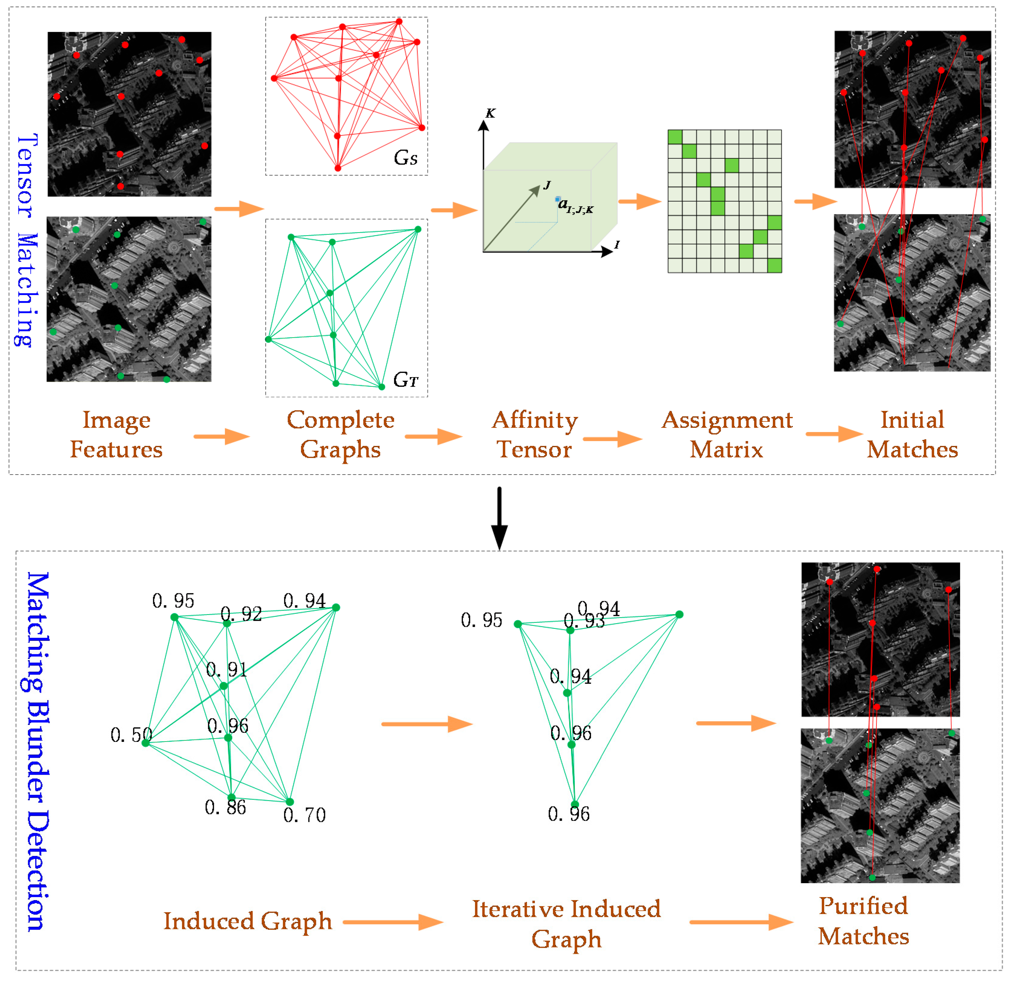
Given a source and target images acquired from different sensors, image matching aims to find point correspondences between the two images. The proposed method for matching involves a four-step process, namely complete graph building [
32], affinity tensor construction, tensor power iteration and matching gross error detection. In the first stage, an upgraded FAST detector (named uniform robust FAST, abbreviated as UR-FAST, which will be detailed in
Section 2.2) was used to extract image features, and two complete graphs in both source and target images are built with their nodes representing FAST features. Then, the affinity tensor between the graphs is built with its elements expressing the node similarities. Next, the tensor power iteration is applied to obtain the leading vector which contains coarse matching results. Finally, a gross error detection method is followed for purifying the matching results.
Figure 2 shows the main process of the proposed method.
2.1. Definition of the Affinity Tensor
Given a source and a target image,
and
are the two image feature point sets extracted from the source and target image, respectively; the numbers of features in
and
are
m and
n;
(
) and
(
) are feature indices of
and
;
and
are the two complete graphs built by
and
(as illustrated in
Figure 2). In the mathematical field of graph theory, a complete graph is a simple undirected graph in which every pair of distinct nodes is connected by a unique edge. As we can see from
Figure 2, there are ten and eight features in the source and target image, respectively. According to the complete graph theory, there are
unique edges that connect node pairs in
, and
unique edges that connect node pairs in
.
The affinity tensor
is built on the two complete graphs (
and
) which describes the similarity of the two graphs. In this paper, tensor
can be considered as a three-way array with a size of
, i.e.,
and
is a tensor element located in column
I, row
J and tube
K in the tensor cube (as shown in
Figure 2). To explicitly express how the tensor elements are constructed, we use (
i,
i′), (
j,
j′) and (
k,
k′) to replace
I,
J, and
K. The indices
i,
j, and
k are feature indices in the source image ranging from 0 to
m − 1;
i′,
j′ and
k′ are feature indices in the target image ranging from 0 to
n − 1. In this way, the tensor element
is rewritten as
located at (
i ×
n +
i′) column, (
j ×
n +
j′) row, and (
k ×
n +
k′) tube, and it expresses the similarity of triangles
and
which are the two triangles in graph
and
, respectively.
The tensor element
can be computed by Equation (1):
where
and
are the geometric descriptors of
and
. As shown in
Figure 3, the geometric descriptors are usually expressed as the cosines of the three vertical angles in a triangle (i.e.,
). The variable
represented the Gaussian kernel band width;
is the length of a vector; and
is a balanced factor which will be detailed below.
As shown in Equation (1), triangle
and
will degenerate to a pair of points when
and
; thus,
and
will be radiometric descriptors (e.g., 128 dimensional SIFT descriptor or 64 dimensional SURF descriptor) of image feature
and
. However, the geometric descriptors are related to cosines of angles, and the radiometric descriptors are related to intensity of image pixels; the two kinds of descriptors have different physical dimensions. In addition, the radiometric descriptors are more distinctive than geometric descriptors because the radiometric descriptors have higher dimensions than those of the geometric descriptors. To balance the differences of physical dimensions and descriptor distinctiveness, Wang et al. [
30] suggested normalizing all the descriptors to a unit norm.
However, a simple normalization can only alleviate the physical dimensional differences. Thus, a constant factor
is used to balance the differences of descriptor distinctiveness. In this way, the geometric and radiometric information are equally important when encoded in the affinity tensor. The constant factor
can be estimated by the correct matches of image pairs in prior:
where
and
are the average distances of normalized radiometric and geometric descriptors, respectively.
Though the balanced factor differs in different image pairs, they have the same order of magnitude. The order of magnitude of can be estimated as follows:
- (1)
Select an image pair from the images to be matched, extract a number of tie points manually or automatically (the automatic matching method could be SIFT, SURF, and so on);
- (2)
Remove the erroneous tie points by manual check or gross error detection algorithm such as Random sample consensus (RANSAC) [
33];
- (3)
Estimate the average feature descriptor distance of the matched features, named ;
- (4)
Construct triangulated irregular network (TIN) by the matched points, and compute the average triangle descriptor distance of the matched triangles, named ;
- (5)
Compute the balanced factor with Equation (2).
In practical matching tasks, calculating for every image pair is very time consuming and unnecessary, and only the order of magnitude of is significant. Thus, we sample a pair of images from the image set to be matched, estimate the order of magnitude of , and apply this factor for the rest of image pairs. The configuration of also has some principles in tensor matching: if both geometric and radiometric distortions are small, then can be an arbitrary positive real number because either geometric or radiometric information is sufficient for matching; if geometric distortions are small, then it is preferable a greater because radiometric information should be suppressed in matching; if radiometric distortions are small, then a smaller would be better because large geometric distortions will contaminate the affinity tensor if not depressed.
2.2. Construction of the Affinity Tensor
The affinity tensor of two complete graphs can be constructed by Equation (1). Whereas a pair of images may consist of thousands of image features, and using all the features to construct a complete tensor is very memory and time consuming, sometimes a partial tensor is sufficient for matching. Besides, the feature repeatability is relatively low in multi-sensor remote sensing images, thus leading to small overlaps between feature sets. In addition, the outliers of image features mix with inliers and introduce unrelated information in the tensor which leads to a local minimum in power iteration [
34]. Moreover, to speed up tensor power iteration, the affinity tensor should maintain a certain sparseness. Based on the above requirements, the following four strategies are proposed to construct a small, relatively pure and sparse tensor.
(1) Extracting high repetitive and evenly distributed features. Repetitiveness of features is a critical factor for a successful matching [
2]. We evaluated common used image features such as SIFT, SURF, and so on, and found that FAST feature had the highest feature repetitiveness. As mentioned in
Section 2.1, the measure of structural similarities of the graph nodes are three inner angles of the triangles. However, if any two vertices in a triangle has a small distance, then a small shift of a vertex may lead to tremendous differences of the inner angles. Consequently, noises are introduced in computing tensor elements. Inspired by UR-SIFT (uniform robust SIFT [
35]), we design a new version of FAST named UR-FAST to extract evenly distributed image features. As shown in
Figure 4, the standard FAST features are clustered in violently changed textures, while the modified FAST features have a better distribution. It should be noted that UR-FAST detector is only applied in the source image, and the features in the target image are acquired by standard FAST and approximate nearest neighbors (ANN) [
36], which will be detailed in strategy (2).
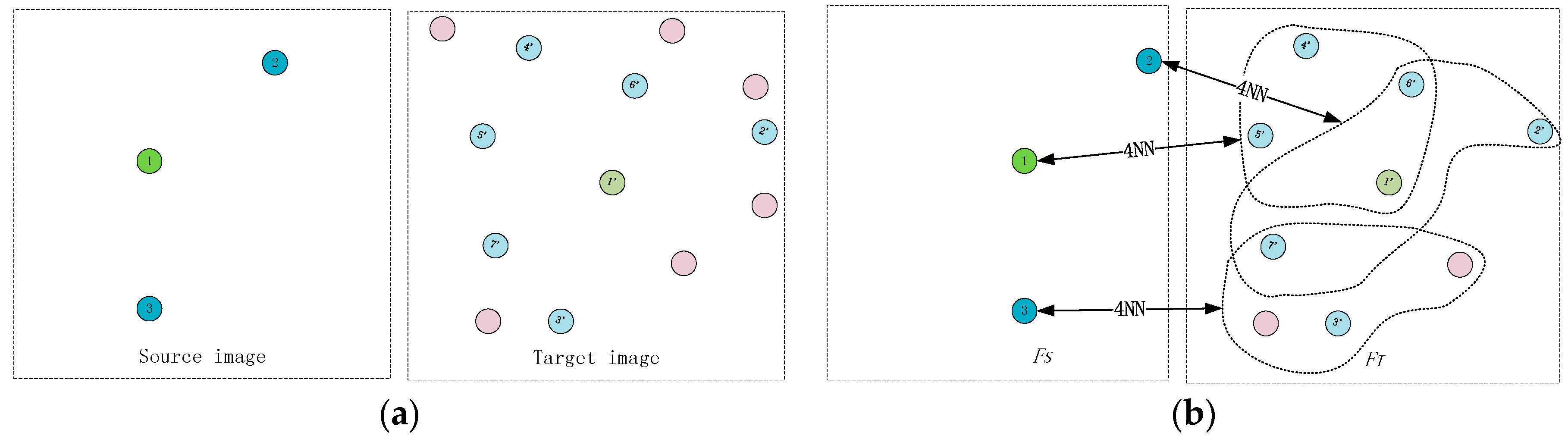
(2) Reducing the number of image features. The detected features are filtered by ANN [
36] searching algorithm for constructing two feature sets
and
. As illustrated in
Figure 5a, there are 3 UR-FAST features and 13 FAST features in the source and target images, respectively. As shown in
Figure 5b, to guarantee feature repetitiveness, for every feature element in
, ANN searching algorithm is used to search its 4 most probable matches among the 13 features in the target image. All the candidate matches of feature elements in
constitute
(as shown in
Figure 5b, the original feature number in target image is 13, while the feature number decreases to 9 after filtering). In this way, the tensor size decreases to (3 × 9)
3 from the original size of (3 × 13)
3, which sharply decreases the memory consumption.
(3) Computing a partial tensor. When using the definition of an affinity tensor in Equation (1), the tensor element
means the geometric similarity of
and
. As described in strategy (2), (3 × 9)
3 elements should be computed for the complete tensor. Actually, completely computing the tensor will be redundant and make the tensor less sparse. Therefore, in this algorithm, only a small part of the tensor elements is computed. As shown in
Figure 6, to compute a partial tensor, the ANN searching algorithm is applied once again to find the 3 most similar triangles in
for
(As shown in
Figure 6,
,
, and
are the searching results). That is, the tensor elements
,
, and
are non-zero, and the remaining tensor elements are zero. In this way, the effects of outliers are alleviated, and the tensor is much sparser.
(4) Making the graph nodes distribute evenly. Though UR-FAST makes image features distribute evenly, there is still some possibility that triangles in the graphs occasionally have small areas, and the vertices of the triangles are approximately collinear. Thus, a threshold of 15 pixels is set to make the triangles have relatively large areas. If a triangle in either graph has an area fewer than 15 pixels, then all the tensor elements related to this triangle are set to zero. Formally, if , then ; if , then . The threshold (15 pixels) has less relationship with sensor types, and it is not case specific but more of an empirical value. Since UR-FAST avoid clustered image features, the area constraint condition is seldom violated unless the triangle vertices are approximately collinear.
2.3. Power Iteration of the Affinity Tensor
In the perspective of graph theory, the feature correspondence problem is to find the maximum similar sub-graphs (i.e., maximize the summation of the node similarities). The best matching should be satisfied by
where
is the assignment matrix,
indicates that
are the indices of matched points;
is the vectorization of
;
is a vector with all elements equal to 1.
The constraint term in Equation (3) shows that all the elements in and are less than 1, i.e., every node in has at most one corresponding node in , and every node in has at most one corresponding node in (that is, the node mapping between and is an injective mapping).
Equation (3) actually is a sub-graph isomorphism problem, with no known polynomial-time algorithm (it is also known as an NP-complete problem [
37]). However, the solution of Equation (3) can be well approximated by the leading vector of the affinity tensor which can be obtained by tensor power iteration [
34]; the interpretation is as follows.
Based on Equation (1), if
is bigger, then the possibility that
and
are matched triangles is higher, and vice versa. Thus, the tensor elements can be expressed with probability theory under the assumption that the correspondences of the node pairs are independent [
37]:
where
is the matching possibility of feature pair
i and
i′.
Equation (4) can be rewritten in a tensor product form [
38]
where
is the vector with its elements expressing the matching possibility of feature pairs;
is the tensor Kronecker product symbol; and
is a tensor constructed by two graphs that have no noise or outliers, and all the node correspondences are independent.
Though in practical matching tasks, noise, and outliers are inevitable, and the assumption that the node correspondences are independent is weak, the matching problem can be approximated by the following function
where
is the operator of Frobenius norm.
Though the exact solution of Equation (3) generally cannot be solved in polynomial-time, it can be well approximated by Equation (6), of which the computational complexity is O((mn)3). The tensor power iteration is illustrated in Algorithm 1.
| Algorithm 1: Affinity tensor power iteration. |
 |
The output of Algorithm 1 is the leading vector of the tensor
A (i.e., the solution to Equation (6)). The size of the affinity tensor
A is
(i.e., the tensor has
mn columns,
mn rows, and
mn tubes), so
p*, the leading vector of the tensor
A, has the length of
mn. Besides, the elements of the tensor
A are real numbers, so the elements of
p* are real numbers too. To obtain the assignment matrix, we should firstly transform
p* to a
matrix (the matrix is called soft assignment matrix because its elements are real numbers. In the manuscript, we donate by
Z), then discretize
Z to
Z* by use of greedy algorithm [
39] or Hungarian algorithm [
40]. Finally, the correspondences of image features are generated by the assignment matrix
Z*.
2.4. Matching Blunder Detection by Affinity Tensor
Though the aforementioned tensor matching algorithm gets rid of most of the mismatching points, there are still matching blunders caused by outliers, image distortions, and noise. Thus, this paper proposed an affinity tensor-based method for eliminating erroneous matches.
The proposed method is based on the observation that the structures among images are relatively static. Meanwhile, the affinity tensor includes structural information of the image features. Therefore, the two matched graphs can induce an attributed graph. In the induced graph, every node has an attribute that is computed by the summation of the similarities of the triangles which include such a node. As shown from
Figure 7,
and
are two matched graphs including six pairs of matched nodes, and the node pair 6 and 6′ is an erroneous correspondence. Therefore, in this induced graph, the node induced by erroneous matched node pair (i.e., node 6 in
, which is induced by node pair 6 and 6′) has a small attribute which measures the similarity that comes from other nodes. In a more formal expression, the attribute of induced node
i can be expressed as follows
where
is the attribute of node
i in
;
and
,
and
, and
and
are the matched node pairs; and
N is the number of the matched triangles.
Equation (7) is the basic formula for matching blunder detection. In a practical matching task, the number of the blunders is more than illustrated in
Figure 7, and it is very hard to distinguish blunders from noise. Thus, we embed Equation (7) in an iterative algorithm: the big blunders are eliminated first and then the small ones until the similarities are kept constant. The algorithm is illustrated in Algorithm 2.
In Algorithm 2, I, J, K are the abbreviations for feature index pairs (i,i’), (j,j’) and (k,k’); p represents for p-th iteration. c is a constant; it can be calculated by the average similarity of triangles which constructed by two error-free matched feature set (the calculating formula is shown in Equation (7)). In this paper, it is empirically set to 0.85.
| Algorithm 2: Blunder detection by the affinity tensor. |
 |
To verify the effectiveness of Algorithm 2, it was compared to RANSAC algorithm integrated with a homographic transformation (the threshold of re-projected errors was set to 3.0 pixels). The results are shown in
Figure 8.
As can be seen from
Figure 8a, 30 pairs of evenly distributed tie points are selected from the sub-image pairs. To verify the robustness of the two algorithms, from 10 to 100 pairs of randomly generated tie points are added in the matched feature sets as the matching blunders. Two parameters are used to evaluate the effectiveness of the algorithms. The first one is
rf (
rf =
fp/
t), where
fp is the number of falsely detected blunders (that is, the detected matching blunders are actually correct matches, the detection algorithm falsely mark them as erroneous matches),
t is the total number of correctly matched points. In this experiment,
t is 30. In the ideal case,
rf is 0, as a lower
rf indicates a better algorithm. The other parameter to measure the usefulness of the algorithms is
rc (
rc =
ct/
g), where
ct is the number of correctly detected blunders and
g is the total number of matching blunders in the matched points; in this experiment,
g varies from 10 to 100. By the experimental results,
rc of RANSAC and tensor-based algorithms was 1.0, this means both algorithms detected all the gross errors. The results of
rf were demonstrated in
Figure 8b. Although both algorithms can detect all the blunders, the tensor-based algorithm seems to perform better than RANSAC because the average
rf of the former one is only 0.03, which is far below that of the latter. The essence of RANSAC is randomly sampling, the global geometric transform model is fitted by the sampled points, and the rest of the points are treated as verification set. The drawback of RANSAC is that the probability of correct sampling is very low when encountered with considerable mismatches, and finally RANSAC is stuck in a local minimum. However, graph-based detection method avoids these drawbacks, because the node attributes represent other nodes’ support. If the node is an outlier, other nodes’ support will be very small, and thus the attribute indicates whether the node is an outlier or not.
3. Experimental Results
The proposed ATBM was evaluated with five pairs of images which were captured by ZY-3 backward (ZY3-BWD), ZY-3 nadir (ZY3-NAD), GF-1, GF-2, unmanned aerial vehicle (UAV) platform, Jilin1 (JL1), SPOT 5, and SPOT6 sensors. To examine its effectiveness, five descriptor-based matching algorithms were chosen as the competitors, namely, SIFT, SURF, NG-SIFT, OR-SIFT, and GOM-SIFT. These five descriptor matching algorithms were state-of-the-art in matching multi-sensor images. The matcher for these algorithms was ANN searching, and the NNDR threshold was set to 0.8. In the following, evaluation criteria, experimental datasets, implementation details, and experimental results are presented.
3.1. Evaluation Criterion and Datasets
In order to evaluate the proposed method, two common criteria including recall and precision [
10] were used. The two criteria are defined as follows: recall =
CM/
C and precision =
CM/
M, where
CM (correct matches) was the number of correctly matched point pairs,
C (correspondences) was the total number of existing correspondences in the initial feature point sets, and
M (matches) was the number of matched points. However, for large images covering mountainous and urban areas, a global transformation such as projective and second-order polynomial models could not accurately express the geometric transformation among such images [
18]. Thus, in the estimation of
C and
CM, 25 pairs of sub-images grabbed from the complete image pairs were used for evaluation. Each of the sub-image pairs was typically characterized by non-linear intensity differences and considerable textural changes (the details of the complete image pairs were listed in
Table 1; the sub-image pairs were shown in
Figure 9).
C and CM were determined as follows: A skilled operator manually selected 10–30 evenly distributed tie points between image pairs, and an accurate homographic transformation was computed using the selected tie points. Then the computed homographic matrix with the back-projective error threshold of 3.0 pixels was used to determine the number of correct matches and correspondences.
Apart from recall and precision, positional accuracy was used to evaluate the matching effectiveness of ATBM and other five matching algorithms. The positional accuracy was also used by Ye and San [
18] and was computed as follows. First, TIN was constructed using the matched points of the complete image pair, and 13–38 evenly distributed checkpoints (or CPs, for short) were fed to the Delaunay triangulation. Then, an affine transformation model was fitted by the matched triangles. Lastly, positional accuracy was estimated via the root mean square error (RMSE), which was computed through the affine transformation of the CPs.
3.2. Implementation Details and Experimental Results
In the process of feature extraction, UR-FAST was applied in the source image, and standard FAST was used in the target image. It was shown by our experiments that this feature extracting strategy could greatly improve the feature repetitiveness compared to commonly used feature detectors such as Harris features, BRISK, DoG, and ORB. In the construction of the affinity tensors, to guarantee repetitive rate of image feature, it retained 50 UR-FAST features in the source image. For every UR-FAST feature, ANN algorithm was applied to search for its 4 candidate correspondences; for every triangle in the source image, ANN algorithm was applied again to search for its 3 candidate matched triangles (by our experiments, the matching recall reached the peak when the numbers of candidate matching features and triangles were 4 and 3, respectively). The Gaussian kernel bandwidth in Equation (1) was set to , and any computed tensor elements that were higher than were set to zero. The balanced weighted factor in Equation (1) was empirically set to 0.01 (the more precise balanced weighted factor could be calculated by Equation (2) if necessary). Besides, to trade off computational cost and accuracy, we made 5 trials in power iterations (the power iteration was shown in Algorithm 1).
The complete image pairs listed in
Table 1 were the testing datasets for estimating positional accuracy. There were thousands of feature points in these image pairs. Thus, computing the affinity tensors for such image pairs was very time consuming. Meanwhile, storing all the feature descriptors in computer memory was nearly impossible. Therefore, SIFT algorithm (SIFT algorithm was optional; other algorithms such as SURF and ORB were also sufficient for the coarse matching) was used to obtain some tie points in down-sampled image pairs. Then, we roughly computed the homographic transformation between the image pairs. Next, the two images of an image pair were gridded to sub-image pairs, and every sub-image pair would be overlapped under the constraint of the homographic transformation (this coarse-to-fine strategy was also applied by the compared algorithms). In the end, all the sub-image pairs were matched by ABTM as illustrated in
Figure 2.
ABTM, SIFT, SURF, NG-SIFT, OR-SIFT, and GOM-SIFT were also evaluated with the testing data listed in
Table 1. All the test image pairs were selected from different sensors and, hence, had considerable illumination differences particularly in images with higher resolution. In addition, these test images had different scales and topographic relief, so obvious geometric distortions and considerable texture changes were present.
Figure 10 showed the matching results of ABTM on the five test image pairs. It seemed clear that ABTM obtained favorable matching results though there were non-linear intensity differences with considerable texture changes and somewhat obvious geometric distortions.
As shown in
Figure 10, ATBM obtained abundant and evenly distributed matches in all of the experimental images. The first pair of images was from Xinjiang, China and captured by GF-1 and ZY-3 sensors; therefore, the illumination differences were obvious as evidenced by the matching details. Besides, there were also changes in scale caused by the differences of ground sampling distance (GSD) of sensors and the vast topographic relief caused by the Chi-lien Mountains. These two factors resulted in locally non-linear intensity differences and geometric distortions. Nevertheless, ATBM obtained evenly distributed tie points in the sub-image pairs (as shown in
Figure 10f). However, in the middle of the first image pair (
Figure 10a), there was no tie point. This is because the two images were captured at different moments, and the image textures changed dramatically. Thus, there was hardly any feature repetition. Although feature correspondences by geometric constraints are found in the initial matching process, the tensor-based detection algorithm eliminated all the false positive matches in the gross error detection process of ATBM.
The second image pair consisted of two images from the GF-2 and ZY-3 sensors. The two images were captured at different moments which spanned over three years; therefore, considerable textural changes were presented as a result of the rapid development of modern cities in China (as shown
Figure 10g). The tie points of the second sub-image pair were clustered in unchanged image patches because ATBM detected feature correspondences using radiometric and geometric constraints. It could find feature matches in the unchanged textures which were surrounded by numerous changed textures. Therefore, the tie points of the complete image pair (as shown in
Figure 10b) distributed well.
The third pair of images was captured by the ZY3-BWD and ZY3-NAD sensors. The two images were taken in different seasons—namely early spring and midsummer. The different seasons led to much severer intensity changes compared to the first two image pairs. For example, it seemed clear that in
Figure 10h, some of the pixel intensity was reversed. However, ATBM was immune to intensity changes and obtained stable matching results in this image pair as well.
The fourth pair of images was shot by UAV and JL1 sensors (the camera equipped on UAV platform was Canon EOS 5D Mark III), and it could be seen that JL1 image was blurrier than UAV image. The transmission distance between the sensed target and satellite sensors was much longer than that of UAV sensors and their targets, the reflected light lost more in the transmission, thus the UAV images looked sharper than satellite images. Besides, as in the second image pair, the two images were captured at different seasons. JL1 image was covered by thick snow, while the UAV image was covered by growing trees (as shown
Figure 10i). However, both these two challenges had few impacts on the matching results, and ATBM still obtained abundant tie points.
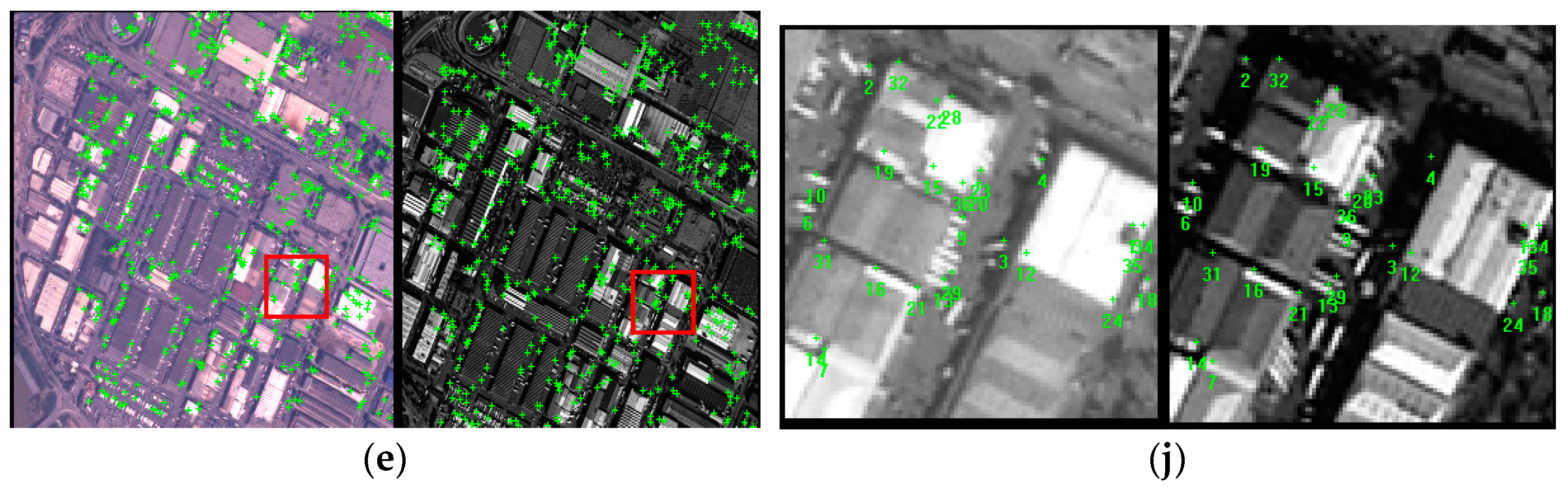
The fifth pair of images was from an urban area and the image resolution was high (2.5 m for SPOT5 and 1.5 m for SPOT6), and the two images were characteristic with structured textures (as shown in
Figure 10j). These textures benefitted FAST corner detector, and thus the matching result was satisfied too.
Figure 11 gave a quantitative description of ATBM and a comparison of the five feature descriptors. ATBM outperformed the other five matching algorithms in all the evaluation criterion including matching recall, matching precision, number of correct matches, and positional accuracy.
ATBM outperformed the other five algorithms in all the test images which contained locally non-linear intensity differences, geometric distortions, and numerous textural changes. The better performance owed to the higher matching recall (higher than 0.5 in matching recall for ATBM as shown in
Figure 11a), which resulted in more correct matches between image pairs. In addition, ATBM used the affinity tensor-based gross error detection algorithm which could distinguish true matches among a number of wrong ones. Thus, the matching precision and the number of correct matches was higher too (the average number of correct matches for ATBM was approximately 20 for sub-image pairs). Higher positional accuracy (an average of 2.5 pixels for ATBM) was consequent because positional accuracy was mainly determined by the number of correct matches and matching precision.
ATBM tended to match feature points with the similarities in both geometry and radiometry. Both geometric and radiometric information played the same role in matching texturally fine and well-structured images (i.e., images with small geometric and radiometric distortions). The higher matching recall benefitted from the affinity tensor which encoded geometric and radiometric information. Geometry described the intrinsic relations of feature points. Meanwhile radiometry represented local appearances. When geometric or radiometric distortions were considerable, ATBM could make the two constraints compensate for each other. For example, in sub-image pair 1, the geometric distortions were relatively large, and thus, radiometric information played a leading role in matching. While in sub-image pair 3, the flat farmlands resulted in relatively small geometric distortions, and such information compensated for the radiometric information in matching.
In general, descriptor-based matching algorithms are determined via NNDR of the radiometric descriptors. When encountered with non-linear intensity differences and changed textures, the drawback of the NNDR strategy in matching multi-sensor images was exposed: descriptor distance of two matched features was insufficiently small. OR-SIFT and GOM-SIFT modified the descriptor to adapt the textures in which the radiometric intensity differences were reversed, while these image pairs were not such the case because the intensity differences were non-linear. NG-SIFT used normalized descriptors and abandoned gradient magnitude, though it had a certain of capability to resist non-linear intensity differences, it had problems in descriptor distinctiveness. Therefore, the descriptor-based matching methods such as SIFT, SUFR, OR-SIFT, GOM-SIFT and NG-SIFT had relatively lower matching recall in the experimental image pairs. ATBM avoided NNDR rule and tended to find the best matches in geometry and radiometry, and thus leading to higher matching recall. Benefitting from higher matching recall, there were more correct matches for ATMB in the sub-image pairs (shown in
Figure 11c), and it could also be concluded that there would be more correct matches in the complete image pairs (evidences were shown in
Figure 10a–e). With more correct matches, the positional accuracy was higher, too (as shown in
Figure 11d).
The experimental results of the five descriptor-based matching algorithms were strongly dependent on the image contents: GOM-SIFT obtained the most correct matches and highest matching recall (
Figure 11a,b), SIFT had the best matching precision (
Figure 11c). In most cases, OR-SIFT and GOM-SIFT had similar matching results, because OR-SIFT used the same manner as GOM-SIFT to build feature descriptors; the differences between them were that OR-SIFT had the half-descriptor dimensions of GOM-SIFT, thus OR-SIFT had efficiency advantage in ANN searching. SIFT had the best matching precision in the experimental data; this is because SIFT descriptor had higher distinctiveness than another four feature descriptors. NG-SIFT and SURF had no obvious regularity in the testing data, though both of them were characteristic with scale, rotation, and partly illumination change invariance, which were also the capabilities of SIFT, OR-SIFT, and GOM-SIFT.
ATBM outperformed other five matching algorithms again in positional accuracy (shown in
Figure 11d). Positional accuracy was mainly determined by the matching precision, number of correct matches and their spatial distribution. In most cases, more numbers of correct matches (as we can see from
Figure 11b, ATBM had more numbers of correct) meant a better spatial distribution, and the matching precision of ATBM was higher than other five algorithms too (shown in
Figure 11c). Therefore, ATBM had higher positional accuracy than other five descriptor matching algorithms.
4. Conclusions and Future Work
Image matching is a fundamental step in remote sensing image registration, aerial triangulation, and object detection. Although it has been well-addressed by feature-based matching algorithms, it remains a challenge to match multi-sensor images because of non-linear intensity differences, geometric distortions and textural changes. Conventional feature-based algorithms have been prone to failure because they only use radiometric information. This study presented a novel matching algorithm that integrated geometric and radiometric information into an affinity tensor and utilized such a tensor to address matching blunders. The proposed method involved three steps: graph building, tensor-based matching, and tensor-based detection. In graph building, the UR-FAST and ANN searching algorithms were applied, and the extracted image features were regarded as graph nodes. Then the affinity tensor was built with its elements representing the similarities of nodes and triangles. The initial matching results were obtained by tensor power iteration. Finally, the affinity tensor was used again to eliminate matching errors.
The proposed method had been evaluated using five pairs of multi-sensor remote sensing images covered with six different sensors: ZY3-BWD, ZY3-NAD, GF-1 and GF-2, JL-1 and UAV platform. Compared with traditionally used feature matching descriptors such as SIFT, SURF, NG-SIFT, OR-SIFT and GOM-SIFT, the proposed ATBM could achieve reliable matching results in terms of matching recall, precision correct matches, and positional accuracy of the experimental data. Because the tensor-based model is a generalized matching model, the proposed method can also be applied in point cloud registration and multi-source data fusion.
However, a few problems should be addressed in future research. The bottleneck of the computing efficiency is ANN algorithm when using in the searching for n most similar triangles. For example, if a feature set consists of 50 image features, these features constitute 503 triangles, then the KD-tree will have 503 nodes, and lead to a very time-consuming result for construction of KD-tree. In addition, the efficiency of searching for n most similar triangles in a 503 nodes KD-tree is very low in essence. The computational time of ATBM is higher than that of SURF, SIFT because the considerable size of the affinity tensor increased computing operations in the power iterations. Further research can introduce new strategies to make the tensor sparser and reduce computational complexity in power iterations. Besides, power iterations also could be implemented in a GPU-based parallel computing framework which could immensely speed the power iterations.


