Multitemporal Cloud Masking in the Google Earth Engine

Abstract

The exploitation of Earth observation satellite images acquired by optical instruments requires an automatic and accurate cloud detection. Multitemporal approaches to cloud detection are usually more powerful than their single scene counterparts since the presence of clouds varies greatly from one acquisition to another whereas surface can be assumed stationary in a broad sense. However, two practical limitations usually hamper their operational use: the access to the complete satellite image archive and the required computational power. This work presents a cloud detection and removal methodology implemented in the Google Earth Engine (GEE) cloud computing platform in order to meet these requirements. The proposed methodology is tested for the Landsat-8 mission over a large collection of manually labeled cloud masks from the Biome dataset. The quantitative results show state-of-the-art performance compared with mono-temporal standard approaches, such as FMask and ACCA algorithms, yielding improvements between 4–5% in classification accuracy and 3–10% in commission errors. The algorithm implementation within the Google Earth Engine and the generated cloud masks for all test images are released for interested readers.

1. Introduction

Reliable and accurate cloud detection is a mandatory first step towards developing remote sensing products based on optical satellite images. Undetected clouds in the acquired satellite images hampers their operational exploitation at a global scale since cloud contamination affects most Earth observation applications [1]. Cloud masking of time series is thus a priority to obtain a better monitoring of the land cover dynamics and to generate more elaborated products [2].

Cloud detection approaches are generally based on the assumption that clouds present some useful features for their identification and discrimination from the underlying surface. On the one hand, a simple approach to cloud detection consists then in applying thresholds over a set of selected features, such as reflectance or temperature of the processed image, based on the physical properties of the clouds [3,4,5,6]. Apart from its simplicity, such approaches produce accurate results for satellite instruments that acquire enough spectral information, but it is challenging to adjust a set of thresholds that work at a global level. On the other hand, there is empirical evidence that supervised machine learning approaches outperform threshold-based ones in single scene cloud detection [1,7,8,9]. For instance, Ref. [1,7,9] show that neural networks are good candidates for cloud detection. However, they present practical limitations since they need a statistically significant, large collection of labeled images to learn from. This is because, in order to design algorithms capable of working globally over different types of surfaces and over different seasons, a huge number of image pixels labeled as cloudy or cloud free must be available to train the models. This labelling process usually requires a large amount of tedious manual work, which is also not exempt from errors. Furthermore, additional independent data has to be gathered to validate the performance of the algorithms, which increases the data requirements and dedication. In any case, both threshold and machine learning based cloud detection algorithms relying only on the information of the analyzed image are still far from being perfect and produce systematic errors specially over high reflectance surfaces such as urban areas, bright sand over coastlines, snow and ice covers [10].

In this complex scenario, including temporal information helps to distinguish clouds from the surface, since the latter usually remains stable over time. Cloud detection methodologies can thus be divided into monotemporal single scene and multitemporal approaches. Single scene approaches only use the information from a given image to build the cloud mask, while multitemporal approaches also exploit the information of previously acquired images, collocated over the same area, to improve the cloud detection accuracy. Multitemporal cloud detection is therefore an intrinsically easier problem because location and features of clouds vary greatly between acquisitions, whereas the surface is to a certain extent stable. However, multitemporal methods are computationally demanding, and the lack of accessibility to previous data usually hampers their operational application to most satellite missions. Therefore, in order to exploit the wealth of the temporal information, long-term missions with a granted access to the satellite images archive, and suitable computing platforms, are required. A clear example fulfilling these requirements is the Landsat mission from NASA [11], which provides global image data over land since 1972. For this reason we will focus here on Landsat images, although the methodology and the subsequent discussion can also be applied to other similar satellites [12].

There exists a wide variety of multitemporal approaches for cloud detection that have been applied to Landsat imagery [13,14,15,16,17,18,19]. In the Multitemporal Cloud Detection (MTCD) algorithm [14], the authors use a composite cloud-free image as reference, then they detect clouds by setting a threshold on the difference between the target and the reference in the blue band. In order to reduce false positives, they use an extra correlation criteria with at least 10 previous images. In Ref. [15], a previous spatially collocated cloud-free image from the same region is manually selected as the reference image. Then a set of thresholds over the reflectance in some Landsat bands (B1, B4 and B6) and over the difference in reflectance between the target and the reference image are set. The Temporal mask (TMask) algorithm [16] builds a pixel-wise time series regression to model the cloud-free reflectance of each pixel. It uses the FMask algorithm [5] to decide which pixels to include in such a regression model. Then, it applies a set of thresholds over the difference in reflectance between the estimated and the target image in Landsat bands B2, B4 and B5. The work presented in Ref. [17] is also based on FMask. In this case, they first remove one of the FMask tests to reduce over-detection, and compute the FMask cloud probability for each image in the time series. Afterwards, they compute the pixel-wise median FMask cloud probability and the standard deviation over the time series. Then, analyzed pixels are masked as cloudy if (a) the modified FMask says it is a cloud; or (b) if the cloud probability exceeds 3.5 standard deviations the median value. Recently, Ref. [19] proposed to also use a composite reference image and a set of thresholds over the difference in reflectance between the target and the reference in Landsat bands B3, B4 and B5. Thus the method is similar to the one presented in Ref. [14] but without the correlation criteria over the time series. Finally, in Ref. [18], we modeled the background surface from the three previous collocated cloud-free images using a non-linear kernel ridge regression that minimizes both prediction and estimation errors simultaneously. Then, the difference image between this background surface reference and the target is clustered and a threshold over the mean difference reflectance is applied to each cluster to decide if it belongs to a cloudy or cloud-free area. In summary, one can see how most of the multitemporal cloud detection schemes proposed in the literature cast the cloud detection problem as a change detection problem [20]: a reference image is built using cloud-free pixels and clouds are detected as particular changes over this reference. To decide whether the change is relevant enough, several thresholds are usually proposed based on heuristics.

Three main issues not properly addressed can be identified in all multitemporal approaches proposed so far:

• Data access and image retrieval. Most of the proposed methods assume that a sufficiently long time series of collocated images is available. It is worth pointing out that retrieving the images to build the time series in an easy and operational manner is technically difficult. We need access to the full catalog and powerful enough GIS software to select and co-register the images. We overcome this limitation using the Google Earth Engine (GEE) platform.
• Computational cost. Most of the proposed methods require a sufficiently long time series of images to operate: at least 15 in the case of TMask [16] and at least 10 in the case of MTCD [14]. This is a critical problem if the algorithm cannot be implemented using parallel computing techniques. We again solve this issue ensuring that our algorithm can be implemented on the GEE cloud computing platform.
• Validation of results. A consistent drawback in most cloud detection studies is the lack of quantitative validation over a large collection of independent images. On the one hand, as we have mentioned in the two previous points, if the multitemporal algorithm is computationally demanding and required images are hard to retrieve, it will be difficult to test the method over a large dataset. On the other hand, simultaneous collocated observations informing about the presence of clouds or independent datasets of manually annotated clouds are often not available. Therefore, without a comprehensive ground truth, validation of cloud detection results is usually limited to a visual inspection of the generated cloud masks. In this work we take advantage of the recently released Landsat-8 Biome Cloud Masks dataset [10], which contains manually generated cloud masks from 96 images from different Biomes around the world.

Therefore, we propose a multitemporal cloud detection algorithm that is also based on the hypothesis that surface reflectance smoothly varies over time, whereas abrupt changes are caused by the presence of clouds. Our proposed methodology extends the work we presented in Ref. [18]. In particular, the proposed methodology presented in this paper consists of four main steps. First, the surface background is estimated using few previous cloud-free images that are automatically retrieved from the Landsat archive stored in the GEE catalog. Then, the difference between the analyzed cloudy image (target) and the cloud-free estimated background (reference) is computed in order to enhance the changes due to the presence of clouds. This difference image is then processed to find homogeneous clusters corresponding to clouds and surface. Finally, the obtained clusters are labelled as cloudy or cloud-free areas by applying a set of thresholds on the difference intensity and on the reflectance of the representative clusters.

In addition, the surface background estimated from the previous cloud-free images can be also used to perform a cloud removal (or cloud filling) in the analyzed cloudy image [21,22]. Pixels masked as clouds can be replaced by the estimated surface background at these locations obtaining a completely cloud-free image [23,24]. The improved frequency of the satellite images time series can then be used to better monitor land cover dynamics and to generate more elaborated products.

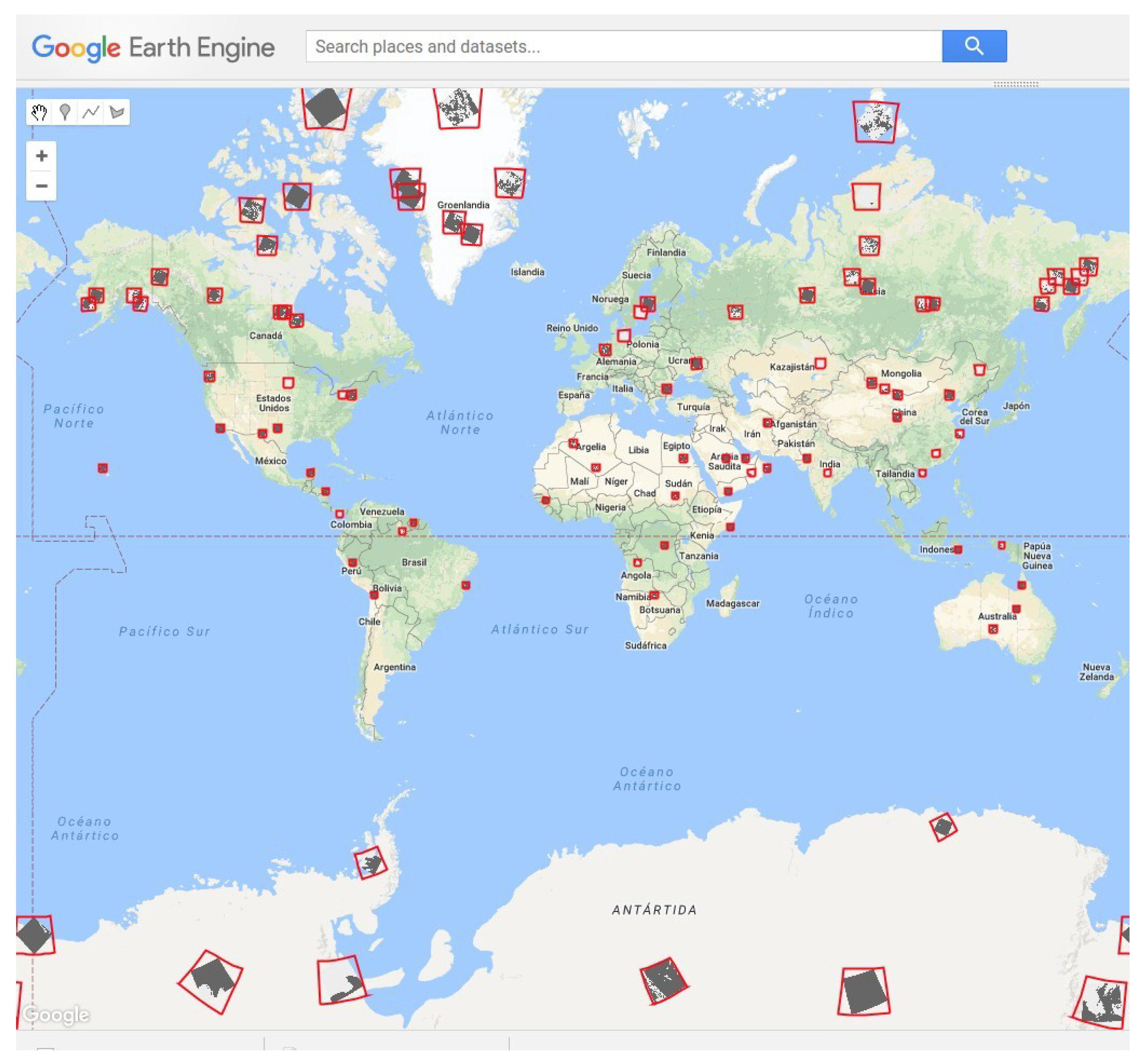
The proposed algorithm is fully implemented in the GEE platform, which grants access to the complete Landsat-8 catalog, reducing the technical complexity of the multitemporal cloud detection and transferring the computational load to the GEE parallel computing infrastructure. The potential of the proposed approach is tested over 2661 500×500 patches extracted from the Biome dataset [10], and the obtained results are available online for the interested readers (http://isp.uv.es/projects/cdc/viewer_l8_GEE.html).

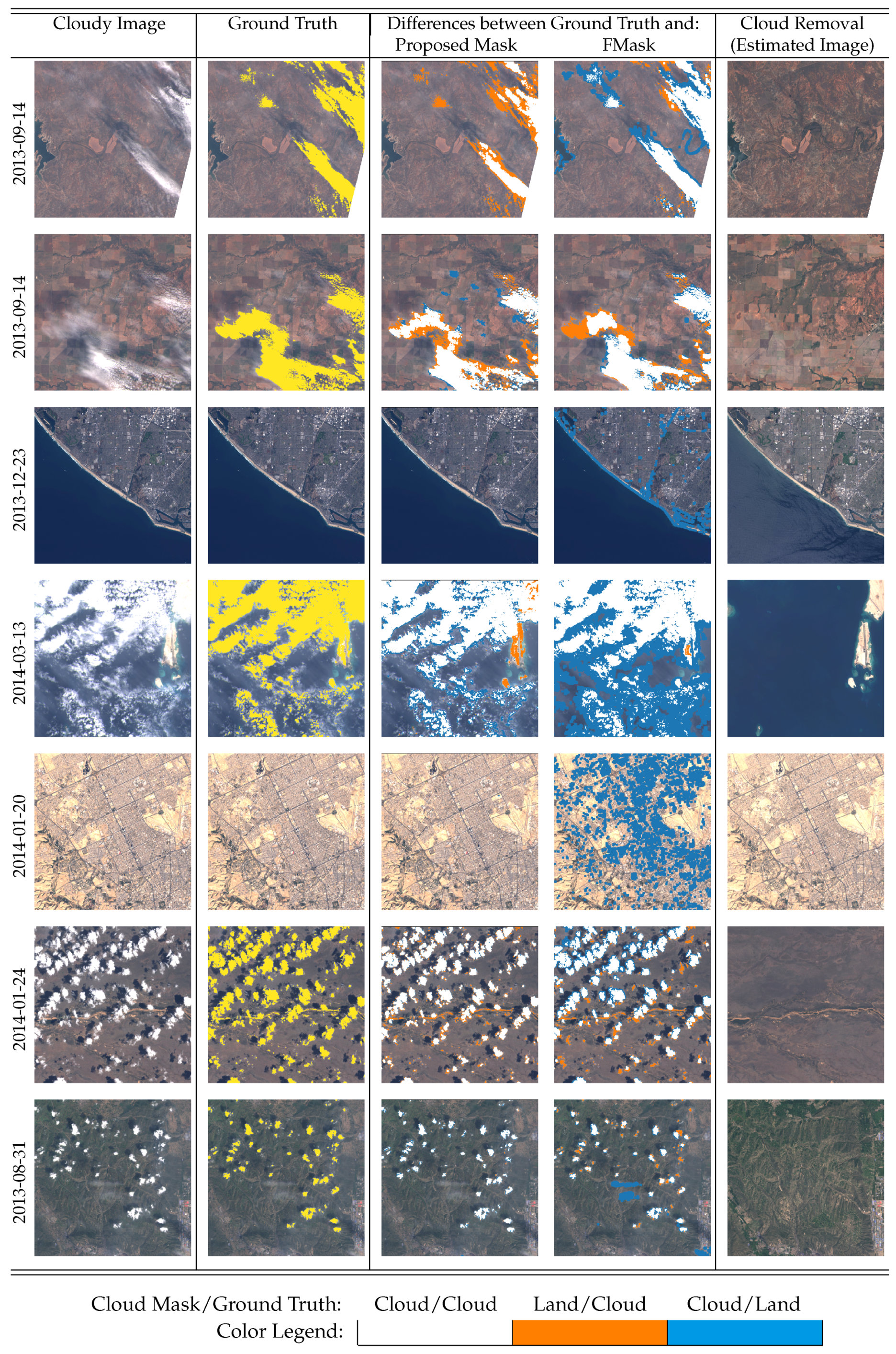
The rest of the paper is organized as follows. In Section 2 the Landsat-8 data, the GEE platform, and the Biome dataset are presented. In Section 3, we explain the proposed methodology for cloud detection and removal. Section 4 presents the evaluation of the proposed methodology. It shows the predictive power of the proposed variables over the dataset, the accuracy, commission and omission errors, some illustrative scenes with the proposed cloud mask, and the cloud removal errors. The algorithm implementation in the Google Earth Engine is briefly described in Section 5. Finally, Section 6 discusses the results and summarizes the conclusions.

2. Satellite Data and Ground Truth

2.1. Landsat-8 Data

The Landsat Program [11] consists of a series of Earth observation satellite missions jointly managed by NASA and the United States Geological Survey (USGS). Landsat is a unique resource with the world’s longest continuously acquired image collection of the Earth’s land areas at moderate to high resolution to support resource assessment, land-cover mapping, and to track inter-annual changes. It started with the first Landsat satellite launched in 1972, and is continued with both Landsat 7 and 8, which are still operational. Landsat 9 is expected to be launched in late 2020 ensuring the Landsat data continuity.

The Landsat-8 payload consists of two science instruments: the Operational Land Imager (OLI) and the Thermal InfraRed Sensor (TIRS), acquiring multispectral images with 11 spectral bands that cover from deep blue to the thermal infrared: B1—Coastal and Aerosol (0.433–0.453 $\mu$m), B2—Blue (0.450–0.515 $\mu$m), B3—Green (0.525–0.600 $\mu$m), B4—Red (0.630–0.680 $\mu$m), B5—Near Infrared or NIR (0.845–0.885 $\mu$m), B6—Short Wavelength Infrared or SWIR (1.560–1.660 $\mu$m), B7—SWIR (2.100–2.300 $\mu$m), B8—Panchromatic (0.500–0.680 $\mu$m), B9—Cirrus (1.360–1.390 $\mu$m), B10—Thermal Infrared or TIR (10.30–11.30 $\mu$m) and B11—TIR (11.50–12.50 $\mu$m). Note that the visible channels are B1-B4 (and B8), which are useful to distinguish the white and bright clouds. Additionally, Landsat-8 presents a band (B9) specifically designed to detect cirrus and high clouds.

2.2. Google Earth Engine Platform

The Google Earth Engine platform [25] is a cloud computing platform for geographical data analysis. It gives access to a full complete catalog of remote sensing products together with the capability to process these products quickly online through massive parallelization. The GEE data catalog includes data from Landsat 4, 5, 7 and 8 processed by the United States Geological Survey (USGS), several MODIS products, including global composites, recently imagery from Sentinel 1, 2 and 3 satellites, and many more. All data are pre-processed and geo-referenced, facilitating its direct use. In addition, user data in raster or vector formats can be uploaded (ingested using GEE terminology) and processed in the GEE. We took advantage of this feature for uploading the manual cloud masks used as ground truth in our experiments.

In this work, all required Landsat images were retrieved from the LANDSAT/LC8_L1T_TOA_FMASK Image Collection available in the GEE. These images consist of top of atmosphere (TOA) reflectance (calibration coefficients are included in metadata [26]). These products also include two additional bands: the quality assessment band (BQA) and the FMask cloud mask [5]. We use the cloud flag included in the BQA nominal product [11] to assess if previous images over each test site location are cloud free or not, which allows us to easily and automatically retrieve cloud-free images from the entire archive. In addition to the Automated Cloud Cover Assessment (ACCA) cloud masking algorithm in the BQA band presented in Ref. [27], the FMask [5] is used to benchmark the proposed cloud detection algorithm. Both algorithms are single-image approaches mainly based on combination of rules and thresholds over a set of spectral indexes.

The GEE computation engine offers both JavaScript and Python application programming interfaces (API), which allow to easily develop algorithms that work in parallel on the Google data computer facilities. The programming model is object oriented and based on the MapReduce paradigm [28]. On the one hand, the GEE engine is accessible through a web-based integrated development environment (IDE) using the JavaScript API. The web-based IDE allows the user to visualize images, results, tables and charts that can be easily exported. On the other hand, the Python API offers the same set of methods, which allow to make requests to the Engine and access the catalog, but without the visualization capabilities of the web-based IDE. However, we chose the Python API to develop our cloud detection scheme because it is easier to integrate with long running tasks, which are essential to run the full validation study in an automatic manner.

2.3. Cloud Detection Ground Truth

Validation of cloud detection algorithms is an extremely difficult task due to the lack of accurate simultaneous collocated information per pixel about the presence of clouds. In this scenario one is forced to manually generate a labeled dataset of annotated clouds, which is time consuming and always includes some uncertainties. Recent validation studies carried out for single scene cloud detection, e.g. for Landsat-8 [10] and for Proba-V [9], are extremely important efforts for the development and validation of cloud screening algorithms. The public dissemination of this data gives the opportunity to fairly benchmark the results on independent datasets and allows to quantify and analyze the cloud screening quality. This is the case of the Landsat 7 Irish dataset [3,29], the Landsat-8 SPARCS dataset [7,30], the Landsat-8 Biome dataset [10,31] or the Sentinel 2 Hollstein dataset [8]. In this work, we take advantage of the Landsat-8 Biome dataset [31] created in Ref. [10]. The Biome dataset consists of 96 Landsat-8 acquisitions (∼7500 × 7500 pixels approximately) from eight different biomes around the world, in which all pixels have been manually labeled. Figure 1 shows the geographic location of the 96 images that form the dataset.

We add these cloud masks with the corresponding Landsat-8 products by ingesting this dataset in the GEE. Then, a few previous cloud-free images for each acquisition were automatically retrieved using the GEE API. From the original 96 Biome products, only 23 of them have enough (three) previous cloud-free images. This is mainly because unfortunately most of the labeled acquisitions selected for the Biome dataset are close to the launch of the Landsat-8 satellite. Therefore, we divided these 23 images in smaller patches of 500 × 500 pixels for our analysis, resulting in 2661 patches.

It is worth noting that validation studies of cloud detection algorithms over large datasets are scarce in the literature and, in the particular case of multitemporal cloud detection, the algorithms have been usually validated on a few images. The use of processing platforms such as the GEE make our study much more feasible.

3. Methodology

The proposed methodology for multitemporal cloud detection is based on our previous work [18]. It works under the assumption that surface reflectance is stable over time or at least follows smooth variations compared to the abrupt changes induced by the presence of clouds. Therefore, this work follows the widespread approach for cloud detection based on multitemporal background modeling with difference change detection extensively used in the remote sensing literature [13,14,15,16,17,18,19]. Figure 2 shows a diagram summarizing the proposed multitemporal cloud detection approach. The following sections describe the main methodological steps.

3.1. Background Estimation

One of the main challenges of the background modeling step is to make it computationally scalable: previous attempts in Ref. [14,16] are computationally demanding, which make them difficult to apply in operational settings. In order to alleviate these problems, in this study we limit the proposed algorithm to work with only three previous collocated images for the surface background estimation. The key for this process to be fully operational is that the selection and retrieval of the three previous cloud-free collocated images has to be carried out automatically. We use the BQA band included in the Landsat products to discriminate if an image is cloud free; and, as we have mentioned, one of the main advantages of using the GEE Python API together with the Landsat image collection is that this step can be fully automated requiring no human intervention.

We call pre-filtering to the first image retrieval step, which consists of assessing if previous images are cloud free or not. Pre-filtering can be solved applying some rough cloud detection method, e.g., setting a threshold over the brightness or over the blue channel as proposed in Ref. [14], or taking advantage of automatic single scene cloud detection schemes if they exist for the given satellite. For this study we use the cloud flag from the Level 1 BQA band of Landsat-8 [27]. We consider an image cloud free if less than $10\%$ of its pixels are masked as cloudy. This raises an important consideration on the design of the cloud detection scheme: it should be robust to errors on the pre-filtering method. An extremely inaccurate pre-filtering algorithm can undermine the performance of the method since cloudy pixels will be used to model the background surface. We will see that these methods are robust enough to work on situations where previous images have some clouds. It is worth pointing out that, since we limit the cloud cover to be less than 10% in each selected image and we assume that clouds are randomly located from one image to another, the probability that the same pixel is cloudy in all three images is expected to be really low.

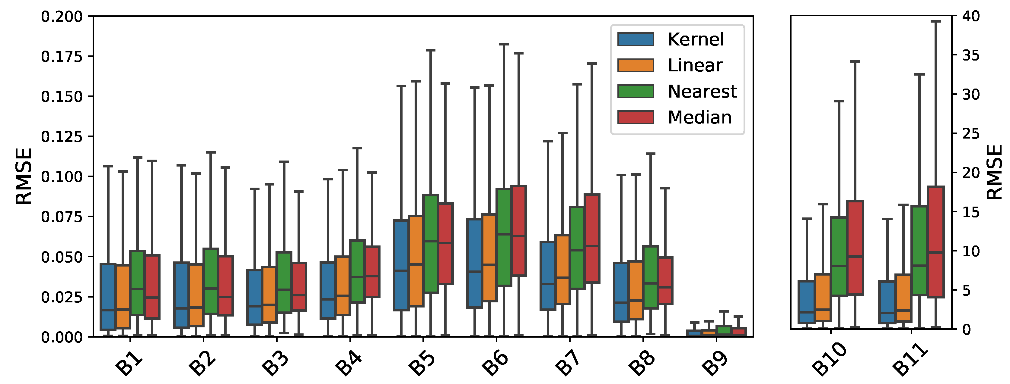
The estimation of the background from the cloud-free image time series is one of the critical steps of the method. We compare four different background estimation methodologies presented in the literature, from simpler to more complex:

• Nearest date: It consists of taking the nearest cloud-free image in time as the background. This is the approach used in Ref. [15], however they rely on human intervention to assess that the image does not present any cloud.
• Median filter: It takes the pixel-wise median over time using the three previous cloud-free images. This is the approach suggested in TMask [16] for pixels where the time series is not long enough.
• Linear regression: It fits a standard regularized linear regression using the time series of the previous cloud-free images [18]. Similarly, TMask [16] used an iterative re-weighted least squares regression at pixel level, which mitigates the effect of eventual cloudy pixels in the time series.
• Kernel regression: The nonlinear version of the former method. It is based on a specific kernel ridge regression (KRR) formulation for change detection presented in Ref. [18].

3.2. Change Detection and Clouds Identification

Once the background is estimated, we use it as a cloud-free reference image to tackle the cloud detection as a change detection problem. Therefore, we compute the difference image between the cloudy target image and the estimated cloud-free reference, which is the base for most change detection methods [20].

However, we do not find changes by applying thresholds directly to the difference image, i.e., target minus estimated. Instead, we previously apply a k-means clustering algorithm over the difference image using all Landsat-8 bands. Afterwards, specific thresholds are applied at a cluster level, i.e., to some features computed over the pixels belonging to each cluster. In particular, we compute three different features for each cluster i: (a) the norm (intensity) of the difference reflectance image over the visible bands (B2, B3 and B4 for Landsat 8), we denote this quantity with ${\alpha }_i$; (b) the mean of the difference reflectance image over visible bands, ${\beta }_i$; and (c) the norm of reflectance image over the visible bands, ${\gamma }_i$. A cluster is classified as cloudy if the three following tests over these features are satisfied: ${\alpha }_i\ge 0.04$, ${\beta }_i\ge 0$ and ${\gamma }_i\ge 0.175$.

The threshold 0.04 on the difference of reflectance image is ubiquitous in the existing literature. For instance, TMask [16] also suggested 0.04 for the B4 channel, MTCD [14] suggests 0.03 on the blue band weighted by the difference between the acquisition time of the image and the reference. The method proposed in Ref. [19] also used 0.04 in the B3 and B4 bands. 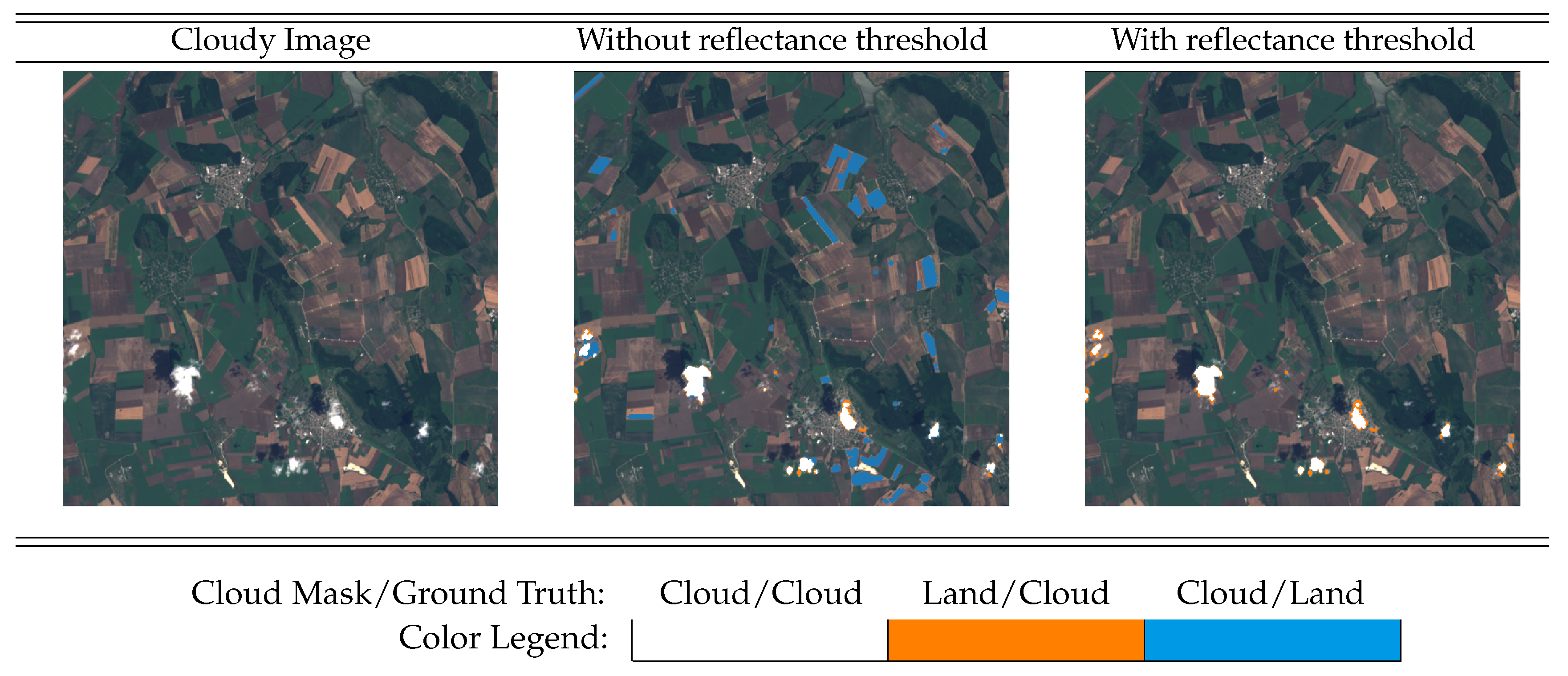In contrast, in our previous work [18] the threshold was higher (0.09) since we used the norm over all the reflectance bands. Here we select the norm as a more robust indicator but restricted to the visible bands (B2, B3 and B4). This threshold is intended to detect significant differences, i.e., with a sufficient intensity to be considered changes, while the other two conditions to be satisfied are specifically included to distinguish clouds from the rest of possible changes in the surface. On the one hand, clouds are usually brighter than the surface so clouds imply an increase in reflectance with respect to the reference background image. By imposing the temporal difference over the visible bands to be positive we exclude intense changes decreasing the reflectance, such as shadows, flooded areas, agricultural changes, etc. On the other hand, we also want to discard changes that increase the brightness but do not look like a cloud in the target image, e.g., agricultural crops. Therefore, we also impose that the norm of the top of atmosphere (TOA) reflectance over the visible bands is higher than 0.175 in order to consider that the cluster corresponds to a cloud. The norm of the visible reflectance bands is also used in Ref. [17] to distinguish potentially cloudy pixels, although in this work they set a lower threshold of 0.15 because they wanted to over-detect cloudy areas.

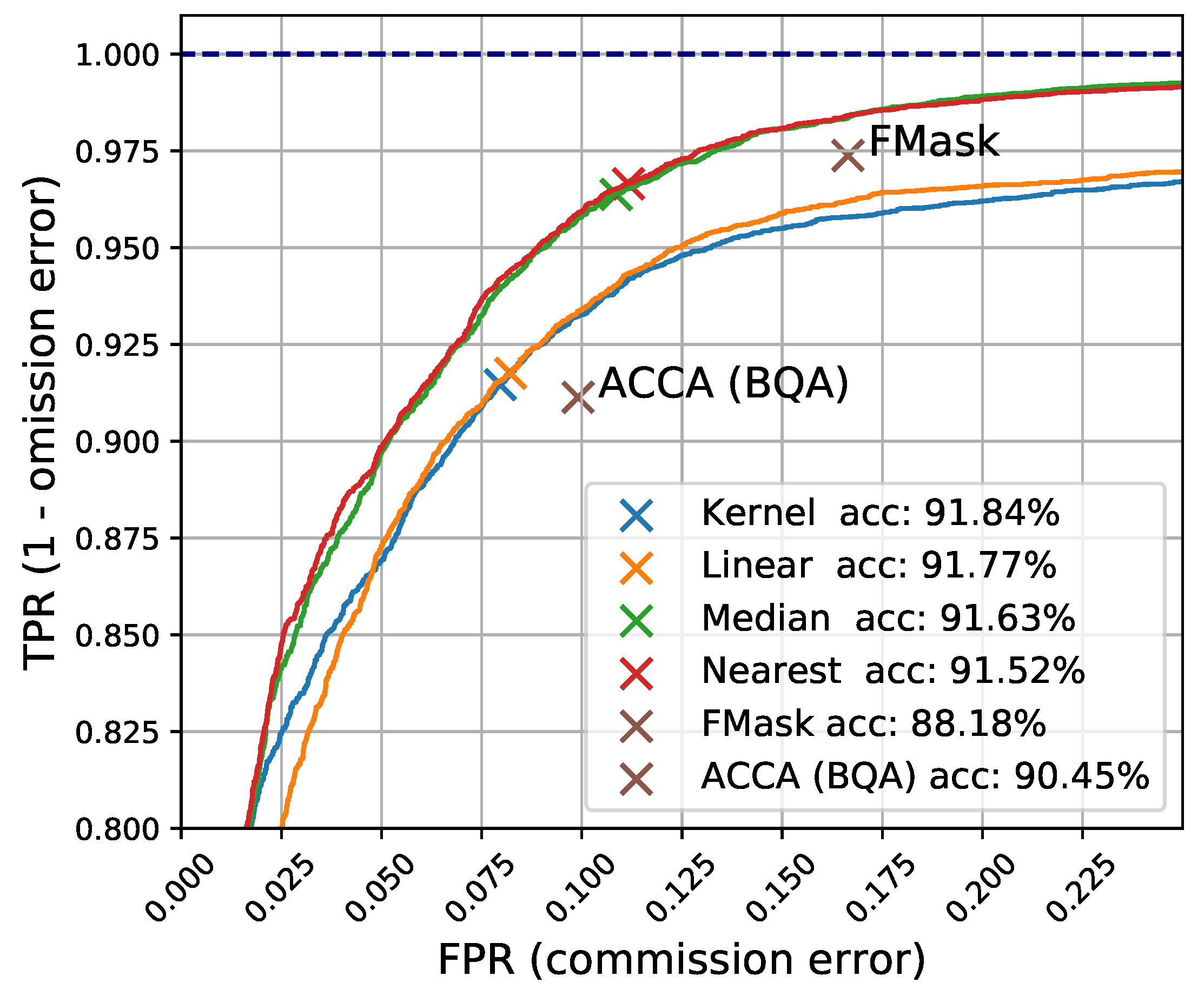
Modifying these thresholds will make the algorithm more or less cloud conservative. We believe that the subsequent user of the cloud mask should have some flexibility to choose to be more or less cloud conservative. For instance, applications like land use or land cover classification are less affected by the presence of semitransparent cirrus whereas for instance estimating the water content of canopy should be much more cloud conservative. Providing the receiver operator curve (ROC) [32] for the entire dataset allows the users to better select these thresholds in order to obtain a trade-off between commission (false positives) and omission (false negatives) errors for their particular application.

3.3. Remarks

One of the main differences of our proposal for cloud detection is the clustering step. We apply a k-means clustering over the difference image over all bands of the satellite. We fixed the number of clusters to 10; this number is related to the size of the image (500 × 500 pixels in the experiments) so if larger images are used this number should be increased. We tried however different numbers of clusters (5, 15 and 20) but we did not observe major differences in performance. The clustering step seeks to capture patterns over all the bands that cannot be captured with a single static threshold. For example, it is well known that the Thermal Infrared Bands (TIR, B10 and B11) have good predictive power for the cloud detection problem. However, setting a global threshold independently of location and season is very difficult since surface temperature greatly varies over places and surfaces. In addition, working with time series exacerbates this problem since the surface temperature might vary quite a lot with the date of the acquired image. Therefore, k-means clustering is intended to group similar patterns, e.g., in temperature, and pixels assigned to the same cluster will be classified afterwards to the same class (cloudy or clear). The clustering step simplifies the problem since instead of classifying pixels we have to classify clusters. However, it might introduce errors in mixed clusters where not all the pixels are purely from one of the two classes (cloudy or clear). In our case, if we classify each cluster according to its majority class using the ground truth, we obtain a classification error lower than 3% for all the proposed background estimation methods in the used dataset. This error can be considered a lower bound of the classification error for the presented results. Finally, it is worth mentioning that if we apply the thresholds directly over the difference image, i.e., without the clustering step, numerical accuracy is not significantly affected, but visual inspection showed less consistency on the masks and higher salt-and-pepper effects.

4. Experimental Results

This section contains the experimental results. First we describe an illustrative example where we show some intermediate results of the method, then the analysis over the full dataset is presented. For these results, we will first explore the parameters and the discriminative power of the multitemporal difference, then we will show the results over the complete dataset for cloud detection and cloud removal.

4.1. Cloud Detection Example

Figure 3 shows the cloud detection results for a cloudy image over Texas (USA). The top right corner shows the RGB composite of the acquired image included in the Biome dataset. We see that it contains several thin clouds scattered across the image. In the bottom left image, the manually labeled ground truth cloud mask (in yellow) from the Biome dataset overlay the RGB composite. We can see here that some very thin clouds are not included in the provided ground truth. The three top left images are the previous cloud-free images retrieved automatically with the GEE API from the GEE Landsat image collection. We see that the top left one is not completely free of clouds: this is because it has less than 10% of clouds according to the ACCA algorithm of the BQA band. The image of the bottom right corner corresponds to the cloud-free estimated background using the median method. We see that this estimation method is robust enough in this case since it has not been affected by the unscreened clouds present in the previous “cloud-free” images, and it correctly preserves other bright surfaces such as urban areas. Finally, we compare both the proposed and the Fmask cloud masks with the available Biome ground truth. The second image of the bottom starting from the left shows the differences between our proposed method and the ground truth. In white it shows the true positives (clouds) of the method with respect the ground truth, in orange the false negatives (omissions) and in blue the false positives (commissions). We see that the overall agreement is very high and most of the discrepancies are on the borders of the clouds. The image to the right corresponds to the differences between FMask and the ground truth, in this case we see that FMask missed some thin clouds in the bottom and in the left part of the image.

4.2. Parameters and Errors Analysis

We evaluate the results in terms of commission errors, omission errors and overall accuracy.

Table 1. Validation metrics: True Positive Rate (TPR), False Positive Rate (FPR), Commission Error, Omission Error, Overall Accuracy.

True Positive Rate	TPR	$\frac{\mathrm{cloudy}\mathrm{pixels}\mathrm{predicted}\mathrm{as}\mathrm{clouds}}{\mathrm{cloudy}\mathrm{pixels}}$
False Positive Rate (Commission Error)	FPR	$\frac{\mathrm{clear}\mathrm{pixels}\mathrm{predicted}\mathrm{as}\mathrm{clouds}}{\mathrm{clear}\mathrm{pixels}}$
Omission Error	1- TPR	$\frac{\mathrm{cloudy}\mathrm{pixels}\mathrm{predicted}\mathrm{as}\mathrm{clear}}{\mathrm{cloudy}\mathrm{pixels}}$
Overall Accuracy		$\frac{\mathrm{cloudy}\mathrm{pixels}\mathrm{pred}.\mathrm{as}\mathrm{clouds}+\mathrm{clear}\mathrm{pixels}\mathrm{pred}.\mathrm{as}\mathrm{clear}}{\mathrm{total}\mathrm{pixels}}$

contains the definition of these metrics. Generally, we can obtain a trade-off between commission and omission errors depending on the requirements. For instance, to reduce the omission error we can reduce the threshold over the reflectance which will make the algorithm more cloud conservative and, as a result, the commission error will increase. On the other hand, if we increase the threshold the commission error will decrease and the algorithm will be more clearly conservative and will probably raise the omission error.

First we want to demonstrate the discriminating capability of the norm of the difference image (${\alpha }_i$) for cloud detection. The receiver operator curve (ROC) shows the true positive rate vs. false positive rate trade-off as we vary the threshold over the predictive variable ${\alpha }_i$. Figure 4 shows four curves corresponding to the four different background estimation methods (nearest date, median filter, Linear regression, and Kernel ridge regression). A cross is displayed for the case of the proposed threshold (0.04). We also show a cross indicating the TPR and FPR values for FMask [5] and for ACCA (BQA) [27] over this dataset. As we see, using the nearest date or the median filter to estimate the background and a single threshold over $\alpha$ we outperform FMask and ACCA (BQA) since those points are below the obtained ROC curves. This means that we can reduce commission error while having the same omission error as FMask, or reduce omission error while maintaining the same commission error as FMask.

It is worth mentioning that the simpler background estimation methods (Median and Nearest) have better performance in terms of cloud detection accuracy. In the case of the median, it is more robust to outliers (e.g., clouds contaminating the images used for the background estimation) than the linear or kernel regression approaches. For the nearest date, it might be because the closer in time the image is, the more similar it is to the target image in terms of surface changes. Nevertheless, we will see in the next sections that the kernel and linear regression methods obtain better results in terms of mean squared error in reflectance and, therefore, will be the more appropriate for the cloud removal task.

Figure 4 shows that using only a threshold over the norm difference has a very good performance on cloud detection. However, as we have mentioned in Section 3.2, by doing this we detect all high differences (changes) in reflectance. Whereas most of these differences are because of the presence of clouds, some of them are due to changes in the surface. Figure 5 shows an example of agricultural crops in Bulgaria. The image on the center shows that some of those fields are detected as clouds if we use only a threshold over the differences.

In order to reduce these false positive cases we added an additional threshold applied directly over the reflectance of the cloudy image instead of over the difference image. In particular, we applied the threshold over the norm of the visible bands, $\gamma$. This is physically grounded since clouds have high reflectance on the visible spectral range. In addition, it has been exploited before in Ref. [17] as a measure of potentially cloudy pixels. Figure 6 confirms this approach. The left plot shows cluster centers colored in orange if the majority of their pixels are cloudy and in blue if most of them are clear. The X-axis shows the norm of the difference in reflectance, $\alpha$, and the Y-axis shows the norm of the reflectance, $\gamma$. We can see that the threshold of 0.04 in $\alpha$ was correctly fixed and that 0.175 is a natural threshold in $\gamma$ for this dataset. The right plot in Figure 6 shows the ROC curves with and without the extra threshold on reflectance $\gamma$. We show the ROC curves corresponding to the thresholds 0.15 and 0.175. We can see that the inclusion of this additional threshold (0.175) increases the overall accuracy from 91 to 94%. The threshold at 0.15 could be used instead of 0.175 for cloud conservative applications. Overall we see that by including this additional restriction (either in 0.175 or 0.15) the resulting algorithm is more accurate and less cloud conservative.

4.3. Cloud Detection Results

Once the parameters and methodology have been fixed we analyze the cloud detection results over the whole dataset.

Table 2. Cloud detection statistics over all pixels of the used Landsat-8 Biome Dataset.

Method	Overall Accuracy	Kappa Statistic	Commission Error	Omission Error
FMask [5]	88.18%	0.7550	16.64%	2.62%
ACCA (BQA) [27]	90.45%	0.7933	9.90%	8.86%
Nearest date	94.18%	0.8733	6.31%	4.87%
Median filter	94.13%	0.8720	6.36%	4.94%
Linear regression	93.66%	0.8593	4.78%	9.32%
Kernel regression	93.56%	0.8572	4.82%	9.53%

shows the cloud detection statistics using both the proposed thresholds for the four background estimation models and for the independent FMask and ACCA (BQA) cloud detection algorithms. We see that multitemporal methods yield higher overall accuracy than single scene methods. In addition, we see that the simpler background estimations, such as the median filter and the nearest date, yield a good trade-off in commission and omission errors. Figure 7 shows the mean accuracy and standard deviation over the patches for each of the 23 Landsat-8 acquisitions. We see here again that the multitemporal approach using the median as background estimator consistently outperforms FMask.

Finally, Figure 8 shows some cherry-picked results of the proposed method using the median to estimate the background. Rows 1, 3 and 5 show some systematic errors of FMask over cities, coastal areas and riversides. Row 2 presents small errors in semitransparent clouds in the middle of the image that are not correctly labeled in the manual ground truth cloud mask but that our method correctly identifies. On the other hand, thin clouds on Rows 1 and 7 are misclassified by the proposed method whereas FMask identifies them correctly. Row 6 again shows errors in the ground truth labels. In this case, a path is falsely identified as a cloud. We found these errors specially over bright surfaces, which remind us that single scene cloud detection is challenging even for human experts. Actually, in some cases, we detected them only because we have previous images from the same location with which to compare. Interested readers can visually inspect cloud detection results and the comparison of both the proposed method and FMask [5] with the Biome ground truth, which are available online at http://isp.uv.es/projects/cdc/viewer_l8_GEE.html for all 2661 patches from the Biome dataset.

4.4. Cloud Removal

In addition to the cloud detection problem, we consider also the task of cloud removal (or cloud filling). Most land applications generally discard cloud contaminated pixels for the estimation of biophysical parameters. In cloudy areas, this causes a big amount of missing values in the processed time series that undermine the statistical significance of the subsequent analysis. In this subsection, we benchmark the different background estimation methodologies proposed in this paper and evaluate their suitability for cloud removal in a large dataset. In Ref. [18], we proposed to use previous images together with the current one to estimate the TOA reflectance of the cloud contaminated areas. This idea is also presented in Ref. [33] using more sophisticated methods, however, our proposal in Ref. [18] can be directly implemented in the GEE platform. We compare these linear and kernel based regression approaches with the two simplest baselines, i.e., using the latest available cloud-free pixel or the pixel-wise median filter. The performance of the cloud removal is quantified and evaluated in terms of the error between the estimated and actual background pixels in the cloud-free areas (since cloud contaminated pixels cannot be compared with the background). The accurate cloud mask and the posterior cloud removal provide cloud-free time series that allow a better monitoring of land cover dynamics and the generation of further remote sensing products. The last column in Figure 8 shows the estimated cloud-free image for some scenes. The plots show the estimated image where clouds have been removed. In fact, we show estimated values for the whole scene and not clouded areas only. We can see how the spatial and radiometric features are well preserved and no cloud residuals can be observed.

Quantitative results for the cloud removal are shown in Figure 9. It shows the distribution of the root mean square error on the 2661 patches separately for each spectral band. In the plots, the mid lines represent the mean RMSE for all the (cloud-free) image pixels, the boxes define the 25 and 75 percentiles of the RMSE distribution, and the vertical lines define the maximum and minimum RMSE values. We see here that the more sophisticated methods for background estimation (Linear and Kernel regression) perform better than the simpler ones (median and nearest). This confirms the results presented in Ref. [18] and shows that estimated reflectance is an accurate option to fill the gaps caused by cloud contamination.

5. Algorithm Implementation in the Google Earth Engine

The data in the GEE platform is organized in collections, usually composed of images or features. Images contain bands (spectra, masks, products, etc.), properties, and metadata. Features can contain any kind of information needed to process data, such as labels for supervised algorithms, polygons to define geographical areas, etc. Users can apply their own defined functions, or use the ones provided by the API, using an operation called mapping, which essentially applies a function over any given collection independently. This allows a straightforward processing of large amounts of images and data in parallel. Using this computational paradigm we implemented the full proposed cloud detection scheme using the Python API. In particular, given an input target image, we map and filter the Landsat-8 LANDSAT/LC8_L1T_TOA_FMASK Image Collection. Then the filtered collection is reduced to produce an Image which is the background estimation. With this reference image we compute the difference image and apply the k-means clustering. Finally, we apply the thresholds as defined in Section 3.

The manual cloud masks from the Biome dataset were ingested in the GEE. Therefore, the proposed methodology together with the comparison with the ground truth is implemented using only the Python API of the GEE platform. The developed code has been published in GitHub at https://github.com/IPL-UV/ee_ipl_uv. In that package we provide a function that computes the cloud mask following the proposed methodology for a given GEE image. In addition, some Python notebooks with examples that go step by step on the proposed methodology have been included in the software package.

Finally, as we have mentioned, in order to show the potential of the GEE platform the proposed algorithms have been tested over 2661 patches extracted from the Biome dataset. The obtained cloud masks can be inspected online for the whole dataset at http://isp.uv.es/projects/cdc/viewer_l8_GEE.html.

6. Discussion

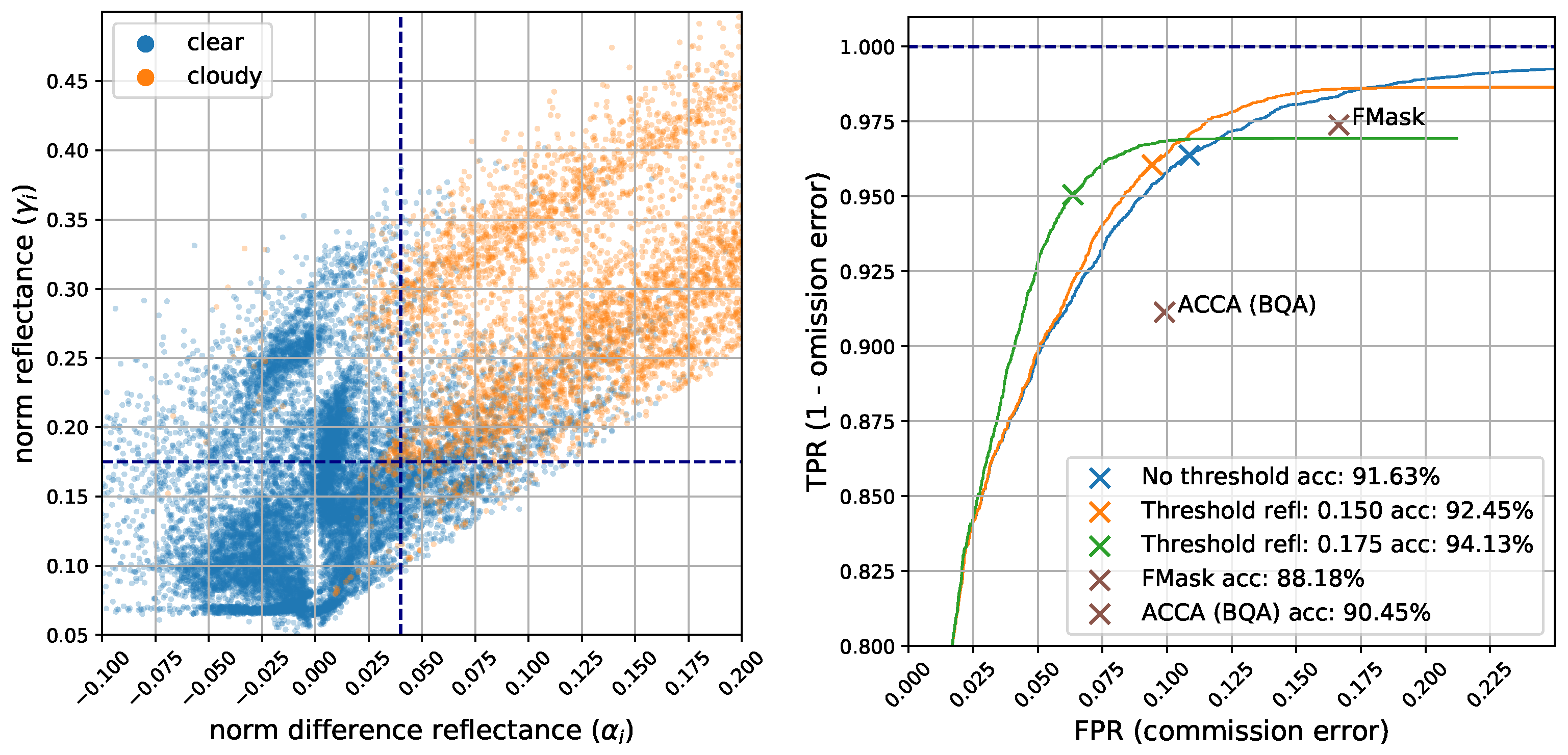
In previous sections we presented a simple yet efficient multitemporal algorithm for cloud detection. The results show an overall increase in detection accuracy and commission error compared to state-of-the-art mono-temporal approaches such as FMask and ACCA. In addition, omission error could be reduced slightly more for the same commission error than FMask using a lower threshold in reflectance ($\gamma =0.15$), as can be seen in Figure 6 (left). For cloud detection, it is normally taken for granted that commission errors are better than omissions, thus operational algorithms tend to overmask in order to avoid false negatives. However, we think that the proliferation of open access satellite image archives implies that in the future more advanced users will be interested in controlling by themselves the trade-off between commission and omission errors depending on their underlying application. To this end, we provide

Table 3. Cloud detection statistics for different thresholds combinations over all selected pixels of the Landsat-8 Biome Dataset, using the median as background estimation method.

Thresholds		Overall Accuracy	Kappa Statistic	Commission Error	Omission Error
Difference ($\mathit{\alpha }$)	Reflectance ($\mathit{\gamma }$)
0.02	0.000	85.54%	0.7076	21.53%	0.95%
0.02	0.150	89.52%	0.7820	15.16%	1.54%
0.02	0.175	92.59%	0.8415	9.61%	3.21%
0.03	0.000	89.56%	0.7823	14.90%	1.93%
0.03	0.150	91.43%	0.8187	11.83%	2.35%
0.03	0.175	93.63%	0.8624	7.76%	3.74%
0.04	0.000	91.63%	0.8217	10.86%	3.63%
0.04	0.150	92.45%	0.8382	9.43%	3.95%
0.04	0.175	94.13%	0.8720	6.36%	4.94%
0.05	0.000	92.50%	0.8378	8.54%	5.53%
0.05	0.150	92.97%	0.8474	7.70%	5.76%
0.05	0.175	94.26%	0.8738	5.32%	6.54%
FMask		88.18%	0.7550	16.64%	2.62%
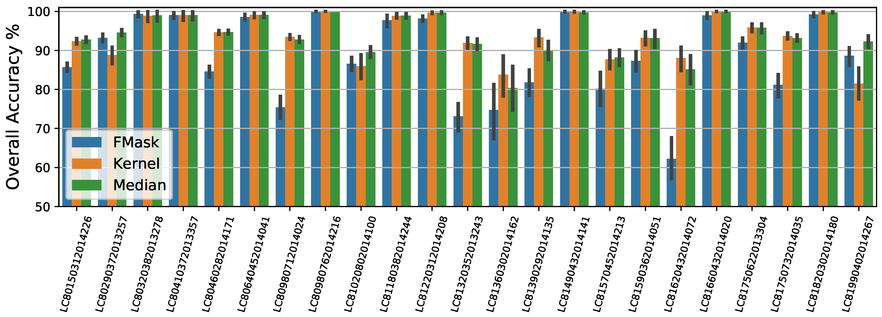
ACCA (BQA)		90.45%	0.7933	9.90%	8.86%

as a guide to help in tuning the thresholds of the current algorithm, where we can see the selected combination providing the best trade-off highlighted in bold. From results shown in Table 2 and Table 3, we can see that the proposed method presents improvements between 4–5% in classification accuracy and 3–10% in commission errors, compared with FMask and ACCA algorithms.

The proposed multitemporal methodology resembles popular multitemporal algorithms such as TMask [16] and MTCD [14] since all of them are based on background estimation and thresholds over the difference image. However, our methodology is simpler and requires less images in the time series to operate. For this reason we consider the current work as a baseline to evaluate trade-offs in processing performance for these more complex multitemporal schemes. It would be of great interest for the community to compare all these approaches in a common benchmark; unfortunately, to this end, we would need labeled images and common open-sourced versions of the algorithms to evaluate the models.

Obviously there are limitations to the proposed multitemporal methodology: for instance, it might fail in situations with sudden changes in the underlying surface, such as permanent snow in upper latitudes. The current dataset lacks these situations, hence we do not recommend its use in such cases.

In addition, another limitation of current and future works on cloud detection is the quality of the ground truth masks: for the Irish dataset [3], the work [34] estimated a mean overall disagreement of 7% over the manual cloud masks labelled by three different experts. The labelling procedure to create the Irish dataset [10] is similar to the Biome dataset that we use in the present work. Therefore, current overall errors are in line with the intrinsic error of human experts following the current labelling procedure. This indicates that in the future, in order to increase the performance, we should develop better labelling methods and provide results by cloud type and underlying surface.

7. Conclusions

In this work, we proposed a multitemporal cloud detection methodology that can be applied at a global scale using the GEE cloud computing platform. We applied the proposed approach to Landsat-8 imagery and we validated it using a large independent dataset of manually labelled images.

The approach is based on a simple multitemporal background modelling algorithm together with a set of tests applied over the segmented difference image, which has shown a high cloud detection power. Our principal findings and contributions can be summarized as follows. This approach outperforms single-scene threshold-based cloud detection approaches for Landsat such as FMask [5] and ACCA (BQA) [27]. We provided an evaluation of different background estimation methods and different variables and thresholds in terms of commission and omission errors. In particular, we showed that simple background detection models such as the median or the nearest cloud-free image are both accurate and robust for the cloud detection task. In addition, for the first time to the authors knowledge, a multitemporal cloud detection scheme is validated over a large collection of independent manually labelled images. The whole process has been implemented within the GEE cloud computing platform and a ready to use implementation has been provided. Compared to previous multitemporal open source implementations, our approach also includes the image retrieval and coregistration steps, which are essential for the operational use of the algorithm. The generated cloud masks can be inspected at http://isp.uv.es/projects/cdc/viewer_l8_GEE.html.

Future lines of research include the application to other optical multispectral satellites requiring accurate and automatic cloud detection. For example, the satellite constellations of Sentinel missions from the European Copernicus programme aim to optimize global coverage and data delivery. In particular, Sentinel-2 mission [12] acquires image time series with a high temporal frequency and unprecedented spatial resolution for satellite missions providing open access data at a global scale. Additionally, another line of research consists of using the multitemporal cloud masks as a proxy of a ground truth that can be used to train single scene supervised machine learning cloud detection algorithms. This approach has been recently successfully applied to image classification tasks [35] and would alleviate data requirements of machine learning methods.

References

1. Gómez-Chova, L.; Camps-Valls, G.; Calpe, J.; Guanter, L.; Moreno, J. Cloud-Screening Algorithm for ENVISAT/MERIS Multispectral Images. IEEE Trans. Geosci. Remote Sens. 2007, 45, 4105–4118. [Google Scholar] [CrossRef] [Green Version]
2. Malenovsky, Z.; Rott, H.; Cihlar, J.; Schaepman, M.E.; García-Santos, G.; Fernandes, R.; Berger, M. Sentinels for science: Potential of Sentinel-1, -2, and -3 missions for scientific observations of ocean, cryosphere and land. Remote Sens. Environ. 2012, 120, 91–101. [Google Scholar] [CrossRef]
3. Irish, R.R.; Barker, J.L.; Goward, S.N.; Arvidson, T. Characterization of the Landsat-7 ETM+ Automated Cloud-Cover Assessment (ACCA) Algorithm. Photogramm. Eng. Remote Sens. 2006, 72, 1179–1188. [Google Scholar] [CrossRef]
4. Zhu, Z.; Woodcock, C.E. Object-based cloud and cloud shadow detection in Landsat imagery. Remote Sens. Environ. 2012, 118, 83–94. [Google Scholar] [CrossRef]
5. Zhu, Z.; Wang, S.; Woodcock, C.E. Improvement and expansion of the Fmask algorithm: Cloud, cloud shadow, and snow detection for Landsats 4–7, 8, and Sentinel 2 images. Remote Sens. Environ. 2015, 159, 269–277. [Google Scholar] [CrossRef]
6. Mei, L.; Vountas, M.; Gómez-Chova, L.; Rozanov, V.; Jäger, M.; Lotz, W.; Burrows, J.P.; Hollmann, R. A Cloud masking algorithm for the XBAER aerosol retrieval using MERIS data. Remote Sens. Environ. 2017, 197, 141–160. [Google Scholar] [CrossRef]
7. Hughes, M.J.; Hayes, D.J. Automated Detection of Cloud and Cloud Shadow in Single-Date Landsat Imagery Using Neural Networks and Spatial Post-Processing. Remote Sens. 2014, 6, 4907–4926. [Google Scholar] [CrossRef] [Green Version]
8. Hollstein, A.; Segl, K.; Guanter, L.; Brell, M.; Enesco, M. Ready-to-Use Methods for the Detection of Clouds, Cirrus, Snow, Shadow, Water and Clear Sky Pixels in Sentinel-2 MSI Images. Remote Sens. 2016, 8, 666. [Google Scholar] [CrossRef]
9. Iannone, R.Q.; Niro, F.; Goryl, P.; Dransfeld, S.; Hoersch, B.; Stelzer, K.; Kirches, G.; Paperin, M.; Brockmann, C.; Gómez-Chova, L.; et al. Proba-V cloud detection Round Robin: Validation results and recommendations. In Proceedings of the 2017 9th International Workshop on the Analysis of Multitemporal Remote Sensing Images (MultiTemp), Brugge, Belgium, 27–29 June 2017; pp. 1–8. [Google Scholar]
10. Foga, S.; Scaramuzza, P.L.; Guo, S.; Zhu, Z.; Dilley, R.D.; Beckmann, T.; Schmidt, G.L.; Dwyer, J.L.; Joseph Hughes, M.; Laue, B. Cloud detection algorithm comparison and validation for operational Landsat data products. Remote Sens. Environ. 2017, 194, 379–390. [Google Scholar] [CrossRef] [Green Version]
11. Loveland, T.R.; Dwyer, J.L. Landsat: Building a strong future. Remote Sens. Environ. 2012, 122, 22–29. [Google Scholar] [CrossRef]
12. Drusch, M.; Bello, U.D.; Carlier, S.; Colin, O.; Fernandez, V.; Gascon, F.; Hoersch, B.; Isola, C.; Laberinti, P.; Martimort, P.; et al. Sentinel-2: ESA’s Optical High-Resolution Mission for GMES Operational Services. Remote Sens. Environ. 2012, 120, 25–36. [Google Scholar] [CrossRef]
13. Wang, B.; Ono, A.; Muramatsu, K.; Fujiwara, N. Automated Detection and Removal of Clouds and Their Shadows from Landsat TM Images. IEICE Trans. Inf. Syst. 1999, 82, 453–460. [Google Scholar]
14. Hagolle, O.; Huc, M.; Pascual, D.V.; Dedieu, G. A multi-temporal method for cloud detection, applied to FORMOSAT-2, VENμS, LANDSAT and SENTINEL-2 images. Remote Sens. Environ. 2010, 114, 1747–1755. [Google Scholar] [CrossRef] [Green Version]
15. Jin, S.; Homer, C.; Yang, L.; Xian, G.; Fry, J.; Danielson, P.; Townsend, P.A. Automated cloud and shadow detection and filling using two-date Landsat imagery in the USA. Int. J. Remote Sens. 2013, 34, 1540–1560. [Google Scholar] [CrossRef]
16. Zhu, Z.; Woodcock, C.E. Automated cloud, cloud shadow, and snow detection in multitemporal Landsat data: An algorithm designed specifically for monitoring land cover change. Remote Sens. Environ. 2014, 152, 217–234. [Google Scholar] [CrossRef]
17. Frantz, D.; Röder, A.; Udelhoven, T.; Schmidt, M. Enhancing the Detectability of Clouds and Their Shadows in Multitemporal Dryland Landsat Imagery: Extending Fmask. IEEE Geosci. Remote Sens. Lett. 2015, 12, 1242–1246. [Google Scholar] [CrossRef]
18. Gómez-Chova, L.; Amorós-López, J.; Mateo-García, G.; Muñoz-Marí, J.; Camps-Valls, G. Cloud masking and removal in remote sensing image time series. J. Appl. Remote Sens. 2017, 11, 015005. [Google Scholar] [CrossRef]
19. Candra, D.S.; Phinn, S.; Scarth, P. Cloud and cloud shadow removal of landsat 8 images using Multitemporal Cloud Removal method. In Proceedings of the 2017 6th International Conference on Agro-Geoinformatics, Fairfax, VA, USA, 7–10 August 2017; pp. 1–5. [Google Scholar]
20. Bovolo, F.; Bruzzone, L. The Time Variable in Data Fusion: A Change Detection Perspective. IEEE Geosci. Remote Sens. Mag. 2015, 3, 8–26. [Google Scholar] [CrossRef]
21. Melgani, F. Contextual reconstruction of cloud-contaminated multitemporal multispectral images. IEEE Trans. Geosci. Remote Sens. 2006, 44, 442–455. [Google Scholar] [CrossRef]
22. Lin, C.H.; Tsai, P.H.; Lai, K.H.; Chen, J.Y. Cloud Removal From Multitemporal Satellite Images Using Information Cloning. IEEE Trans. Geosci. Remote Sens. 2013, 51, 232–241. [Google Scholar] [CrossRef]
23. Hu, G.; Li, X.; Liang, D. Thin cloud removal from remote sensing images using multidirectional dual tree complex wavelet transform and transfer least square support vector regression. J. Appl. Remote Sens. 2015, 9, 095053. [Google Scholar] [CrossRef]
24. Chen, B.; Huang, B.; Chen, L.; Xu, B. Spatially and Temporally Weighted Regression: A Novel Method to Produce Continuous Cloud-Free Landsat Imagery. IEEE Trans. Geosci. Remote Sens. 2017, 55, 27–37. [Google Scholar] [CrossRef]
25. Gorelick, N.; Hancher, M.; Dixon, M.; Ilyushchenko, S.; Thau, D.; Moore, R. Google Earth Engine: Planetary-scale geospatial analysis for everyone. Remote Sens. Environ. 2017, 202, 18–27. [Google Scholar] [CrossRef]
26. Chander, G.; Markham, B.L.; Helder, D.L. Summary of current radiometric calibration coefficients for Landsat MSS, TM, ETM+, and EO-1 ALI sensors. Remote Sens. Environ. 2009, 113, 893–903. [Google Scholar] [CrossRef] [Green Version]
27. Scaramuzza, P.L.; Bouchard, M.A.; Dwyer, J.L. Development of the Landsat Data Continuity Mission Cloud-Cover Assessment Algorithms. IEEE Trans. Geosci. Remote Sens. 2012, 50, 1140–1154. [Google Scholar] [CrossRef]
28. Dean, J.; Ghemawat, S. MapReduce: Simplified Data Processing on Large Clusters. In Proceedings of the Sixth Symposium on Operating System Design and Implementation (OSDI’04), San Francisco, CA, USA, 6–8 December 2004; pp. 137–150. [Google Scholar]
29. U.S. Geological Survey. L7 Irish Cloud Validation Masks; Data Release; U.S. Geological Survey: Reston, VA, USA, 2016.
30. U.S. Geological Survey. L8 SPARCS Cloud Validation Masks; Data Release; U.S. Geological Survey: Reston, VA, USA, 2016.
31. U.S. Geological Survey. L8 Biome Cloud Validation Masks; Data Release; U.S. Geological Survey: Reston, VA, USA, 2016.
32. Fawcett, T. An introduction to ROC analysis. Pattern Recognit. Lett. 2006, 27, 861–874. [Google Scholar] [CrossRef]
33. Meng, F.; Yang, X.; Zhou, C.; Li, Z. A Sparse Dictionary Learning-Based Adaptive Patch Inpainting Method for Thick Clouds Removal from High-Spatial Resolution Remote Sensing Imagery. Sensors 2017, 17, 2130. [Google Scholar] [CrossRef] [PubMed]
34. Oreopoulos, L.; Wilson, M.J.; Várnai, T. Implementation on Landsat Data of a Simple Cloud-Mask Algorithm Developed for MODIS Land Bands. IEEE Geosci. Remote Sens. Lett. 2011, 8, 597–601. [Google Scholar] [CrossRef] [Green Version]
35. Mahajan, D.; Girshick, R.; Ramanathan, V.; He, K.; Paluri, M.; Li, Y.; Bharambe, A.; van der Maaten, L. Exploring the Limits of Weakly Supervised Pretraining. arXiv, 2018; arXiv:1805.00932. [Google Scholar]
Figure 1. Geographic location of the 96 images from the Landsat-8 Biome dataset [31] ingested on the Google Earth Engine.
Remotesensing 10 01079 g001
Figure 2. Multitemporal cloud detection scheme implemented on the Google Earth Engine platform.
Remotesensing 10 01079 g002
Figure 3. Illustration of the Cloud detection scheme. Comparison between the ground truth and the proposed cloud mask algorithm and the FMask. Discrepancies are shown in blue when the proposed method detects ‘cloudy’, and in orange when pixels are classified as ‘cloud-free’.
Remotesensing 10 01079 g003
Figure 4. This figure shows ROC curves for the four proposed background estimation methods. Crosses show the TPR and FPR values for the proposed threshold (0.04) and for FMask [5] and ACCA (BQA) [27] on the same dataset.
Remotesensing 10 01079 g004
Figure 5. Landsat 8 image (LC81820302014180LGN00 006_013) acquired on 10 June 2013. Rural area in Bulgaria presenting crops misclassified as clouds when the threshold in reflectance is not applied.
Remotesensing 10 01079 g005
Figure 6. (Left) Scatter plot of the clusters. Norm of TOA reflectance of the visible bands on the Y-axis ( γ ) and norm of difference in reflectance on the X-axis ( α ). Each point corresponds to one of the 10 clusters from each of the 2661 image patches. Vertical and horizontal lines show the proposed thresholds. (Right) ROC curves with and without the extra threshold on reflectance γ . The median is used for background estimation in both cases.
Remotesensing 10 01079 g006
Figure 7. Average accuracy over the image patches for each of the 23 different Landsat-8 acquisitions selected from the Biome dataset.
Remotesensing 10 01079 g007
Figure 8. Patches of 500 × 500 pixels from Biome dataset. From left to right: RGB scene, RGB scene with ground truth cloud mask in yellow, differences between ground truth and the proposed cloud mask (using the median as background estimation), difference between ground truth and FMask, and estimated cloud-free image.
Remotesensing 10 01079 g008
Figure 9. Root mean square error between the estimated and actual background pixels in the cloud-free areas. Distribution of the errors is shown separately for all Landsat bands for the four background estimation approaches.
Remotesensing 10 01079 g009