Article

Constrained Spectral Clustering of Individual Trees in Dense Forest Using Terrestrial Laser Scanning Data

Swiss Federal Institute for Forest, Snow and Landscape Research WSL, Zürcherstrasse 111, 8903 Birmensdorf, Switzerland
*
Author to whom correspondence should be addressed.
Remote Sens. 2018, 10(7), 1056; https://doi.org/10.3390/rs10071056
Submission received: 26 May 2018 / Revised: 29 June 2018 / Accepted: 2 July 2018 / Published: 4 July 2018
(This article belongs to the Section Forest Remote Sensing)

Abstract

:
The present study introduces an advanced method for 3D segmentation of terrestrial laser scanning data into single tree clusters. It intentionally tackled difficult forest situations with dense and structured tree formations, which inventory practitioners are often faced with. The strongly interlocking tree crowns of different sizes and in different layers characterized the test conditions of close to nature forest plots. Volumetric 3D images of the plots were derived from the original point cloud data. A clustering method with automatically derived priors focused on the segmentation of these images by global optimization. Therefore, each image was segmented as a whole and partitioned into individual tree objects using a combination of state-of-the-art techniques. Multiple steps were combined in a workflow that included a morphological detection of the tree stems, the construction of a similarity graph from the image data, the computation of the eigenspectrum which was weighted with the tree stem priors and the final labelling of the transformed data points in a Markov Random Field framework. The detected trees were verified by number and position which allowed for comparison with other studies. Additionally, for a subset of the data, we provided a detailed verification of the three-dimensional extent of the complete trees. The detection rate by number and position was 97.40% for major trees with a stem diameter at breast height (DBH) ≥ 12 cm and 84.62% for regeneration trees with a DBH < 12 cm. The three-dimensional extent of the detected trees resulted in an average producer’s accuracy of 93.66% and a user’s accuracy of 94.06%. Overall, these numbers confirm the capacity of the method for accurate segmentation of strongly layered and understory trees. Future studies could test the method on wider areas with large scale data and different forest types in order to determine its general transferability.

Graphical Abstract

1. Introduction

Isolating single trees from laser scanning data has been subject of research for forestry related remote sensing since end of the 1980s [1]. A large number of studies exist for both 2D and 3D tree detection, and most of them handle airborne data. For terrestrial laser scanning (TLS) much less studies on automated tree detection have been published. Independent from the sensor’s perspective, the numerous existing studies that dealt with single trees are very different in intention and differ in several ways.
Firstly, an important difference exists between object segmentation and tree modelling. Object segmentation aims at the separation of related parts of a given image which preferably resemble individual objects like trees [2,3,4,5,6]. Typically, the image of several forest trees is segmented as a whole, which is often realized by global optimization techniques. The overall aim is to reach a stable solution for the complete image [3]. As a result, the entire image of the forest is split into clusters of semantically meaningful objects, the individual trees. Modelling of an isolated tree is principally different from object segmentation, as described, for example, by Hackenberg et al. [7] and Raumonen et al. [8]. Modelling aims at the reconstruction of tree geometry. The related trees were previously separated from the point cloud and are often located in relatively loose standing environments [7,9,10,11]. Generally, these approaches are inverse to our clustering approach, since they focus on details of an individual tree instead of the complete image of the forest. These different principles of segmentation and modelling can also be utilized in a complementary way, as it has been demonstrated by Hu et al. [11] and Calders et al. [12]. Both studies sequentially combined segmentation and modelling by prior clustering of the point cloud into point groups of individual trees, before the geometry of each tree was modelled from its cluster.
Secondly, the meaning of single tree detection is used differently in literature and depends on the intended application. In the 2D case, which mostly uses crown height models (CHM) or multispectral imagery from airborne sensors, several approaches determined the tree position at its crown top [6,13,14], while others described the whole circumference of the tree crown [5,15]. In the 3D case, which mostly uses LiDAR point clouds or volumetric imagery, some studies isolated the tree stem but terminologically described it as tree detection [16,17,18], while others aim at isolating the complete tree [19,20,21].
Thirdly, studies refer to different layers of the forest and use data of different forest types and structures. 2D approaches mostly use a perspective from above and are technically only able to separate tree crowns of the upper forest layer [5,6,13]. In addition, 3D approaches which are based on airborne LiDAR, have limitations in detecting understory trees [22,23,24,25]. This is caused by the decreasing signal density of the LiDAR data while penetrating through the canopy [11,21,23,25]. Independent from the sensor’s perspective, tree detection generally yields better results in simple structured and non-dense forest, such as coniferous boreal forest, than in mixed or deciduous temperate forest [22,26,27]. For TLS based approaches, dense and vertically structured forests have only been used for stem detection but not for single tree isolation [28].
This study addresses the shortcomings of individual tree segmentation from high resolution TLS data. It specifically tackles difficult forest environments from plot based terrestrial laser scanning data. For these dense and complex forest conditions, which also include extensive understory, we applied a framework of state-of-the-art 3D image segmentation techniques. To the best of our knowledge, similarly complex forest structures have not yet been used with TLS data for automated 3D tree segmentation. While some initial studies already worked with partly overlapping tree crowns, the overall datasets still appeared to be characterized by well defined mature trees and with little or no understory [10,20,29]. Zhong et al. [30] significantly improved the separation of overlapping tree crowns in the upper canopy layer, but could not distinguish individual trees in vertically layered forest structures. Zou et al. [31] did not extract the complete trees, but only point cloud segments within a defined radius around the stem position that were intended to be used for species classification. Some studies used mobile laser scanning data (MLS) from a moving vehicle to detect and isolate single trees [32,33,34]. However, these studies deal with trees in urban environments, which cannot be compared with complex natural forest structures.
Methodically, many approaches have been used for single tree segmentation. For this study we focused on morphological and machine learning methods for 3D image analysis. After data preprocessing, our overall method consisted of four components. Initially, tree stems were detected using techniques from 3D mathematical morphology. Afterwards, a similarity graph was constructed from the image data which modelled distance relations between the voxels. From this graph, the spectrum of eigenvectors was computed and weighted with the tree stem priors. Final labelling of the data points from the spectrum matrix was conducted in a Markov Random Field framework.
Graph clustering, supported by automatically extracted and labelled tree stem priors, represented the core technique of our method. We adopted a normalized spectral clustering approach, which is an approximation of normalized cut for graph partitioning [35]. While both terms are often used interchangeably, we refer to our relaxed solution as spectral clustering in accordance with the terminology of Von Luxburg [35]. Generally, normalized cut is one of the most widely used types of graph partitioning appoaches and was originally described by Shi and Malik [36] for segmentation of 2D images. Reitberger et al. [21] were the first authors who applied normalized cut for 3D single tree isolation from airborne laser scanning (ALS) data. Since then and despite the demonstrated efficiency, only a few authors used it for tree detection. Hu et al. [11] and Lee et al. [37] likewise applied it on airborne data. For TLS data, this technique was only used by Zhong et al. [30], but their comparatively more simple approach proved to be not capable to separate trees in vertically structured forests. Integrating spectral clustering into a processing framework which manages to deal with complex forest structures captured with high point densities and the different perspective of TLS data is a new challenge of this study.
In comparison to the iterative two-class cut, which was used by Reitberger et al. [21], normalized spectral clustering has advantages in efficiency for multiclass problems [35,36]. It is also known to outperform traditional clustering methods like k-means for many applications [35,38]. However, for challenging segmentation problems, spectral clustering must be supported by high-level information in order to produce semantically meaningful results [38]. This role is typically solved by priors, but implementation into spectral clustering is not straightforward. For the present method, we used the extracted stem objects as priors at two points in the workflow, according to the solutions described by Klein et al. [39], Peluffo-Ordonez et al. [40] and Hu et al. [38].

2. Study Area and Data

2.1. Study Area

The study area was located in mixed and coniferous forest in the canton of Grisons in Switzerland, in the local regions Herrschaft and Schanfigg. It covers varying terrain, ranging form river valleys at low altitudes of 490 m and mountain slopes at an altitude of maximum 1700 m. The forest was generally characterized by close to nature stand structures, and partly serves as protective forest against alpine natural hazards. It is vertically and horizontally structured with diverse layering and considerable amounts of regeneration. The main tree species are Norway spruce (Picea abies L. H. Karst), common beach (Fagus sylvatica L.), silver fir (Abies alba Mill.), European larch (Larix decidua Mill.) and Scots pine (Pinus sylvestris L.). The management regime is close to nature silviculture, which favors natural regeneration by cutting only single trees or small groups.
In this study area, nine square shaped plots were defined with an edge length of 25 m as shown in Figure 1. All plots were centred on permanent sample points of the Swiss national forest inventory (NFI) or the regional inventory of Grisons. The plots were located in diverse forest stands with mostly dense spatial distribution of trees. Concentrated vegetation biomass from foliage and branches often caused visual occlusion effects in the scan data and interlocking crowns increased the overall complexity. Table 1 gives an overview of the local forest characteristics on each plot.

2.2. LiDAR Data

TLS surveys on the individual plots were carried out with a FARO Focus 3D S120 scanner (FARO Technologies Inc., Lake Mary, FL, USA). The scanner used phase shift technology and was configured with a point spacing of 6.14 mm at 10 m distance and an overall resolution of 44 × 10 6 points per scan at a scan size of 10,310 × 4278 points. In order to minimize occlusion effects, five scans were recorded on each plot as shown in Figure 1. All scans were positioned in a so-called corners setup with one scan close to the centre and four scans close to the corners of the plot [41,42]. The exact scan positions were slightly adapted on each plot considering local conditions. For scan registration, six spherical targets were distributed evenly over the plot. The positions of the targets were determined relatively to one long-term global navigation satellite system (GNSS) measurement per plot. Differential correction of these measurements resulted in an average positional accuracy of ±10 cm.
The original point cloud LiDAR data was preprocessed in several steps. Coregistration was done using FARO Scene software (version 5.3, FARO Technologies Inc., Lake Mary, FL, USA) [43] by matching at least three of the spherical targets between each pair of scans. During this process, the geolocation of the targets was used for georeferencing. Further steps included 3D thinning of the point cloud down to 1 point/cm 3 , merging of the single scans, height normalization and clipping to the plot extent. In order to remove other objects from ground vegetation like grass, all datasets were cut at a height threshold of 50 cm above ground [3]. Finally, the point data of each plot was split into quadrants and transferred into a voxel grid. The quadrants were used as data blocks for clustering and contained binary vegetation/background information. They were chosen as the optimal size of a data subset, due to a good trade-off between the requirement to cover the full extent of several trees and to keep the amount of clusters relatively small. Generally, a small number of clusters gives better results, since less options for allocating a node to a cluster exist. The ideal voxel size for tree segmentation was determined to be 10 cm as a trade-off between high resolution and computational effort. The same voxel size was also used by Bienert et al. [20].

2.3. Reference Data

The segmentation results were validated in two ways that required different sets of reference data. As a basic assessment of the detection rates, the number and positions of the detected trees were verified. Validation with this type of reference metrics allowed comparison with other studies, since most of them limit validation to the verification of tree positions only [2,3]. Corresponding references were collected during a field campaign in 2015 and were temporarily close to the TLS measurements. The reference data was acquired for general purposes and not specifically for single tree detection. For mature trees, stem positions at breast height were measured within two concentric circles in accordance with the national forest inventory (see Figure 1). Positions of trees with a stem diameter at breast height (DBH) ≥ 12 cm were recorded within the inner circle of 200 m 2 . In the outer concentric circle of 500 m 2 , only trees with a DBH ≥ 36 cm were measured. For regeneration with a DBH < 12 cm and a minimum crown top height of 130 cm, only a random selection and an arbitrary number of trees per plot were available. Instead of the stem positions at breast height, the crown top positions were collected for these smaller trees. Only for strongly inclined regeneration that had the stem base outside the horizontal projection of the crown area, the positions of the stem base were additionally measured.
In addition to the general validation of tree positions, we developed a procedure to verify the 3D shape and the volume of the isolated trees. The lack of appropriate field reference data prevented previous studies from similarly detailed assessment [11]. We circumvent the problem of missing 3D field references by manually delineating the 3D outline of all trees within a plot quadrant. The original volumetric images served as source data for expert decision based delineation that was technically conducted with the Paraview software suite (version 5.0, Kitware Inc., Clifton Park, NY, USA) [44]. Because 3D delineation was a heavily time-consuming and difficult task, reference data were limited to the first quadrants (Q1) of plots number one, four and five (see Figure 1). Quadrants Q1 of the remaining plots were used to optimize the parametrization of the spectral clustering workflow. The three reference quadrants covered different forest structures and diverse layering of tree sizes for thorough testing of the segmentation. Finally, an isolated volumetric reference object was available for each tree located in these quadrants.

3. Method

3.1. Outline

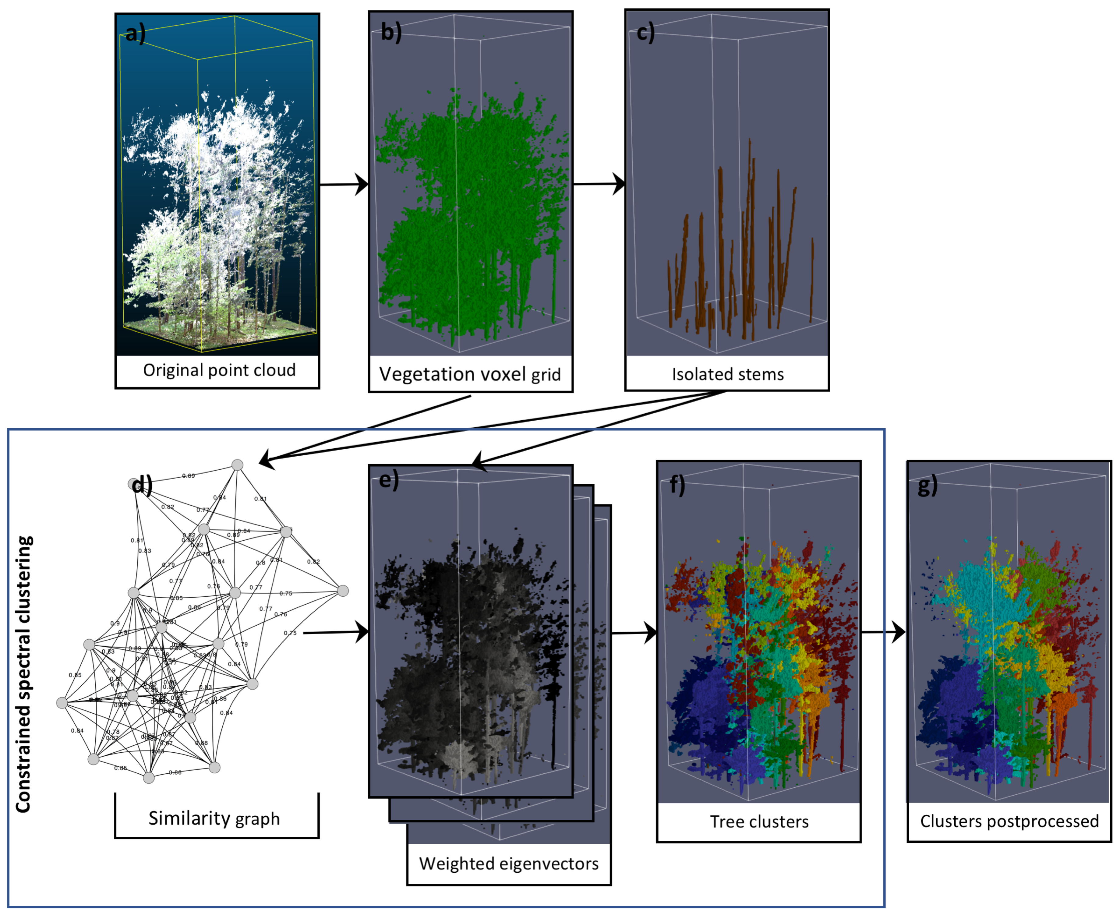
The overall method for individual tree segmentation combined a number of techniques into a comprehensive machine learning framework that was implemented using Python and C/C++ programming languages. The core part of the method was constrained spectral clustering, which was preceded by the extraction of tree stems from the 3D vegetation images. In order to receive semantically meaningful results from spectral clustering, the tree stems were used as priors. Figure 2 shows the general workflow of the method. The major steps are illustrated by visualization of intermediate results using a plot quadrant as an example. The original point cloud in image (a) was preprocessed to the voxel grid in image (b). From this binary image of the vegetation volume, the tree stems were extracted as shown in image (c). Images (d), (e) and (f) of Figure 2 cover the single steps of spectral clustering. Finally, the tree clusters were postprocessed and visualized as labelled image in image (g).

3.2. Tree Stem Detection

Tree stem detection was based on morphological identification of stem candidate segments followed by a logical selection and combination of these segments. The method was recently published by Heinzel and Huber [45], where a detailed description was provided. The fundamentals of the method consisted of a series of 3D opening operations, iteratively using a group of stem templates. The challenge was to remove all image elements that are unlikely to be part of a tree stem and to keep only the stem candidate segments. In terms of mathematical morphology, the stem template served as a structuring element (SE), which was centred on each image voxel and probed the shape and size of its neighbourhood. If the SE fitted into the binary image at this position, the centre voxel was kept. In set theory, morphological opening is expressed like in Equation (1), using the notation of Soille [46]. The opening γ of a set X is a morphological erosion ϵ with the SE B, followed by a dilation δ with the reflected SE B ˇ :
γ B ( X ) = δ B ˇ [ ϵ B ( X ) ] .
The elementary set operations erosion and dilation are defined in Equations (2) and (3), respectively:
ϵ B ( X ) = { x | B x X } ,
δ B ( X ) = { x | B x X } .
The SE played a critical role for stem detection. In order to remove all non-stem image elements, the SE had to constitute a strongly simplified model of a stem. The strict shape of a three-dimensional vertical line clearly reflected the vertically elongated stem profile. In order to consider slight deviations from the vertical orientation, a line of 21-voxel length was stepwise tilted up to a defined degree and rotated around its vertical axis. This resulted in 19 variations of the 3D line, which were successively used as SEs for a series of opening operations. The sum of these individual openings provided the stem candidate segments as connected components. Afterwards, the segments were postprocessed in order to remove noise and atypically shaped objects. Vertically aligned segments were combined to a single stem object in cases when occlusion caused gaps in the stem profile. Due to increased occlusion effects in the upper canopy, it was often not possible to extract the stems to their full extent. Finally, the individual 3D stem objects were received as shown in Figure 2c. Equal parametrisation for morphological opening and postprocessing has been used on all plots and with the values recommended by Heinzel and Huber [45].

3.3. Constrained Spectral Clustering

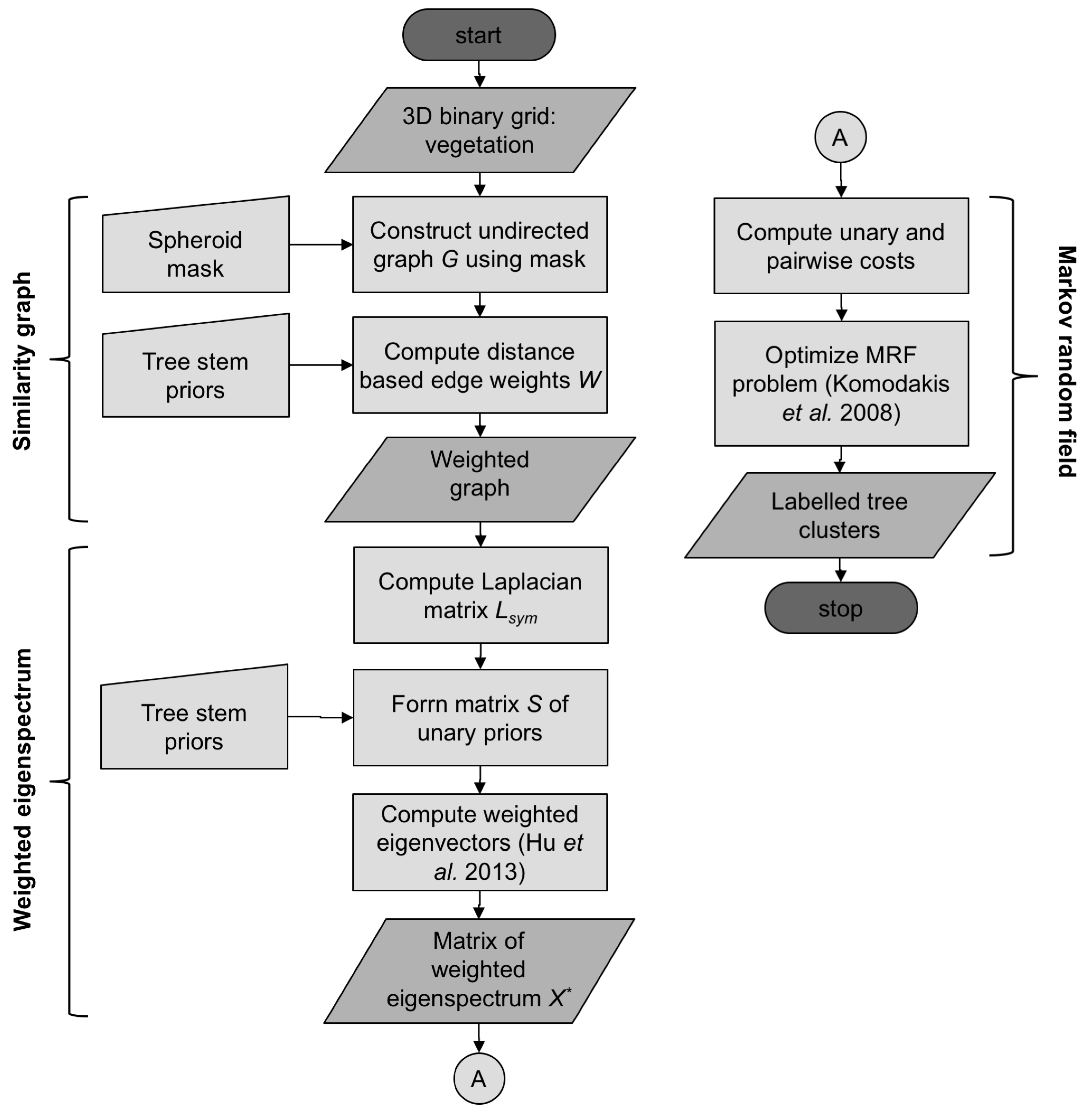
Spectral clustering is the core part of the overall tree segmentation workflow and can be subdivided into three subparts. At first, a similarity graph was built from the image data; then, the weighted eigenspectrum was computed from the graph’s weight matrix and, finally, labelling of the tree clusters was approximated by formulating a Markov Random Field problem. Technically, our spectral clustering approach adapted and combined basic methods described by Von Luxburg [35], Reitberger et al. [21], Hu et al. [38] and Komodakis and Tziritas [47]. The flowchart in Figure 3 provides guidance through the detailed description of the single steps.

3.3.1. Similarity Graph

Spectral clustering is based on modelling the relationship between image elements in the form of an undirected graph G ( V , E , W ) . The vertices V were given by the set of n voxels v 1 , , v n and the edges E indicated connections between the vertices. The similarity between connected pairs was given as a set of weights W, so that each weight w i j refered to the similarity between vertices v i and v j . Because the weights described the likelihood that two voxels belong to the same tree, their design was crucial for clustering performance [21,38].
The weights have been computed solely from distance metrics of the 3D image coordinates. Spectral information, such as intensity of the reflected LiDAR signal or RGB information from photographs, was intentionally dismissed. Due to sensor properties and external illumination, the available spectral information was too inconsistent. For the computation of the distance metrics, we followed the findings of Kamvar et al. [48] and Reitberger et al. [21], but improved them for extended 3D stem information, higher data density from TLS data and for direct inclusion of priors into the edge weights. Three distance related metrics between each pair of voxels i and j (shorthand for v i and v j ) were multiplicatively combined, including the horizontal distance X ( i , j ) , the vertical distance Z ( i , j ) and the 3D-distance T ( i , j ) from the closest stem. Equation (4) defines the computation of the distance weights W d as the product of these components. To limit the computational effort for the high number of voxel pairs in the 3D image, for each voxel i, only those voxels j were considered, that were located within a spheroid of defined size around i. This constitutes the first case condition in Equation (4), which describes a spheroid of horizontal radius r X Y and vertical radius r Z . The horizontal distance between i and j is D i j X Y and the vertical distance is D i j Z . For all other cases, the second condition assigns the distance weight 0 to the graph:
W d ( i , j ) = e X ( i , j ) × e Z ( i , j ) × e T ( i , j ) , if 2 · D i j X Y 2 r X Y 2 + D i j Z 2 r Z 2 1 , 0 , otherwise ,
with
X ( i , j ) = D i j X Y σ x y 2 , Z ( i , j ) = D i j Z σ z 2 , T ( i , j ) = min T i j max σ t 2 .
Equation (5) defines the individual distance factors. The factors X ( i , j ) and Z ( i , j ) provide a weighted metric for the horizontal and vertical distances. The Euclidian distances D i j X Y and D i j Z were weighted by the parameters σ x y and σ z , in order to scale the sensitivity for horizontal and vertical distance separately. This allows better consideration of the vertically elongated shape of trees. The factor T ( i , j ) additionally integrated the pairwise distance from the closest common tree stem. It was computed by determining the maximum distances T i j max of the two voxels i and j from each stem in 3D euclidean space. From these maximum distances, the minimum was selected. In this context, the stem objects were defined as connected components with a 26-adjacency. Intuitively, T ( i , j ) gives a measure of how far the voxel pair is from the closest common tree stem. In addition, this distance factor was weighted by parameters σ t .
For the computation of distance weights, consistent parametrization was used. The radii of the spheroid mask were determined empirically, with the intention to minimize the mask size but avoid drawback for the clustering results. We used the values 0.5 m for r X Y and 3.0 m for r Z . For the distance metrics, the weight parameter values σ x y = 1.35 m, σ z = 11.0 m and σ t = 3.5 m from Reitberger et al. [21] could be adopted and confirmed by testing.
While W d already provided usable weights for the similarity graph, we additionally included knowledge of the stem priors, as defined in Equation (6). Based on the ideas of Peluffo-Ordonez et al. [40] and Klein et al. [39], the final weight w between all voxel pairs i and j was set to 1, if they belonged to the same stem class c in the set of priors P. In case j was part of the priors P, but not of stem class c, w i j was set to 0. This is expressed as the second condition in Equation (6), where P c ¯ = P \ P c . In all other cases, the weight w d i j was kept:
W ( i , j ) = 1 , if v i P c and v j P c , 0 , if v i P c and v j P c ¯ , w d i j , otherwise .

3.3.2. Weighted Eigenspectrum

The next step changed the representation of the data points v i in order to enhance their clustering properties. To achieve this, spectral clustering makes use of the properties of a graph Laplacian matrix as described by Von Luxburg [35]. For the present study, the normalized graph Laplacian was used, which is defined as symmetric matrix L s y m in Equation (7):
L s y m : = D 1 / 2 ( D W ) D 1 / 2 .
The Laplacian was constructed from the weight matrix W R n × n of graph G and the degree matrix D R n × n as the diagonal matrix with the degrees d i = j V w i j on its diagonal. General solutions directly compute the eigenvectors with the m smallest eigenvalues from this graph Laplacian. Then, the rows of the matrix that have the eigenvectors as columns represent the transformed data points.
Differing from this general solution, we additionally incorporated prior information of the tree stems into the eigenvector matrix. Since integration of priors into spectral clustering is not trivial, we applied the method of Hu et al. [38] based on the sample code that is linked in their publication. For details, we refer to this original publication and to the implementation by Lee et al. [37]. Hu et al. [38] showed that the problem of normalized spectral clustering is an optimization of the term
min X tr X T L s y m X , s . t . X T X = I ,
where X R n × m is the label indicator matrix that has to be optimized and I R m × m is the identity matrix. In order to include prior knowledge, this term was modified by introducing a matrix S R n × m that encoded the voxels of the stem priors with one stem per column. This prior information was used in the additional correlation constraint diag ( X T S ) = κ diag ( I ) , with κ being the correlation coefficient. The constraint must be satisfied as a new condition in the modified optimization problem
min X tr X T L s y m X , s . t . diag ( X T X ) = diag ( I ) , X T D 1 / 2 1 = 0 , diag ( X T S ) = κ diag ( I ) .
The columns of the optimized X * are weighted combinations of the eigenvectors. It can be shown that the weight of each eigenvector is proportional to the correlation with the corresponding stem priors. Furthermore, the columns in X * can be regarded as soft indicators for the image voxels belonging to the corresponding tree cluster. Image (e) in Figure 2 visualizes the weighted eigenvectors as image stack, which can be addressed as soft-segmentation according to Hu et al. [38]. Since the row vectors of the optimized X * represented the transformed data points, they were used for final clustering.

3.3.3. Markov Random Fields

Clustering of the data points can be regarded as a problem of optimization of costs and corresponds to minimizing the energy of a Markov Random Field (MRF) [47]. With regards to this, two types of costs were formulated. Firstly, the unary label costs ψ i ( c i ) refer to a label c i that is assigned to a voxel i. Secondly, the separation costs ω i j δ ( c i , c j ) relate to the assignment of labels c i and c j to a pair of voxels i , j , which is connected by a weighted edge in the graph. The latter costs consist of a weight component ω and a function δ for the distances between labels. The two types of costs are combined to the general MRF optimization problem following Komodakis et al. [49]:
arg min c i i V ψ i ( c i ) + ( i , j ) E ω i j δ ( c i , c j ) .
For the present study, the labels corresponded to the stem priors, and the number of labels equaled the number of stems. To solve the clustering problem, we applied the MRF framework for graph segmentation of Komodakis and Tziritas [47] and Komodakis et al. [49]. Hu et al. [38] also used this MRF framework for labelling. In continuance with their method, we used Equations (11)–(13) to compute the unary and the pairwise costs. According to the experiments of Hu et al. [38], η was set to value 2 and X * are the optimized eigenvectors:
ψ i ( c i ) = max ( X i , : * ) X i , c i * ,
ω i j = 1 X i , : * X j , : * 2 2 η ,
δ ( c i , c j ) = γ , if c i c j , 0 , if c i = c j .
Since we worked with nominal labels, a constant value γ for all possible pairs of labels could be used as label distances δ , except for pairs of equal labels that had the distance zero. The costs were precomputed for all voxels and label combinations. For the pairwise potential, only voxel pairs with a 6-adjacency neighbourhood in the original 3D image were considered. Finally, the labels of the data points were received by optimization of the MRF problem and affected the partitioning of the complete 3D image into single tree clusters. The clustering results contained as many tree objects as tree stem priors and are visualized for the sample quadrant in Figure 2f.

3.4. Postprocessing

After computing the labels, automated postprocessing of the tree clusters was performed. The original clusters contained a few typical errors. Due to occlusion effects, small isolated fragments existed that were not connected to the main tree cluster and sometimes labelled incorrectly. This was especially the case in the upper part of the tree crowns, which could only partly be reached by the laser beam from its ground based perspective. Furthermore, tree fragments appeared at the image border, whose related tree stem was completely outside the image.
To remove these errors, postprocessing was limited to simple logical combinations to maintain the transferability to all plots and quadrants. Firstly, all clusters were split into their connected components using 26-adjacency. Those components that included the stem priors were defined as core components. If more than one component per cluster fulfilled this condition, they were combined. The remaining, so-called free components of each label, were allocated to the core component with the smallest three-dimensional Chebyshev distance. This corrected most of the wrongly labelled isolated fragments. Secondly, border effects could be largely eliminated by removing those segments that touched the image border but were not connected to a core component. Furthermore, free clusters without stems that previously touched the ground were removed. The final tree clusters after postprocessing are illustrated as the last step of the workflow in Figure 2g.

3.5. Accuracy Assessment

Two different types of validation were carried out. The first type compared the position and number of detected trees against field reference data. It was conducted on all nine plots including all quadrants. To validate the positions, the automatically derived tree stems were projected onto a horizontal plane. For both, the mature inventory trees and the smaller regeneration trees, geographic coordinates of their positions were compared against the references in a geographic information system (GIS). A match was counted, when the reference position was within the projected stem area or could be clearly assigned without ambiguity. The available types of references for mature inventory trees distinguished between different stem diameters in the inner and outer concentric circles (see Section 2.3 and Figure 1). The positions of the regeneration trees with a DBH smaller than 12 cm were validated in the same way, but, instead of stem reference positions, the crown tops had to be used as an approximation. The positions of the stem feet were only available for a few strongly slanted regeneration trees.
The second approach validated the volume and the three-dimensional extent of the tree clusters. It uses the final clustering results computed with optimized parametrization. The individual parameter values are stated together with the parameter descriptions in Section 3.3.1, Section 3.3.2 and Section 3.3.3. They were determined by processing the quadrants Q1 from the six non-reference plots with different parameter combinations and by visually analysing the results. Afterwards, the quadrants Q1 of the reference plots one, four and five were used for validation. Therefore, the detected tree clusters were compared automatically against the volume and the 3D extent of the manually digitized references. Besides the 3D extent, two special types of error were inspected. In the case that a single reference tree was split into two or more detected clusters containing priors from different stems, it was counted as split error. On the other hand, if a detected cluster clearly merged two or more trees, of which at least one was not represented in the set of stem priors, it was counted as merge error. On some quadrants, small trees of low height above ground formed dense natural clusters in the forest. For these natural clusters, visual separation of single trees was often not possible, and tree stem priors did not exist for several small trees with crown heights about 130 cm or less. In such cases, the natural clusters had to be validated as an entity instead of real tree individuals. Overall accuracies of the 3D extent were computed both as producer’s accuracy and user’s accuracy according to the definition of Congalton [50]. The producer’s accuracy is a measure of omission error and the user’s accuracy a measure of commission error. Both accuracies were calculated in two ways—one time by considering all tree clusters of a quadrant and, another time, only for those tree clusters with an error > 0.

4. Results

Single tree clustering was successfully computed with constant parametrization for all plot quadrants. The results for the detection rates of single trees are given in Table 2. They refer to the positions and the number of trees, but not to the proper extent and volume. The table lists the number of correctly detected trees (auto) versus the number of references (ref) for each plot including all quadrants. Due to the different sets of reference data, results are presented for two groups of mature trees with different minimum DBH and for the available references of the regeneration trees. The overall detection rate for the mature inventory trees with DBH > 12 cm was 97.40% and 97.30% for DBH > 36 cm. Regeneration trees with a DBH < 12 cm have an overall detection rate of 84.62%.
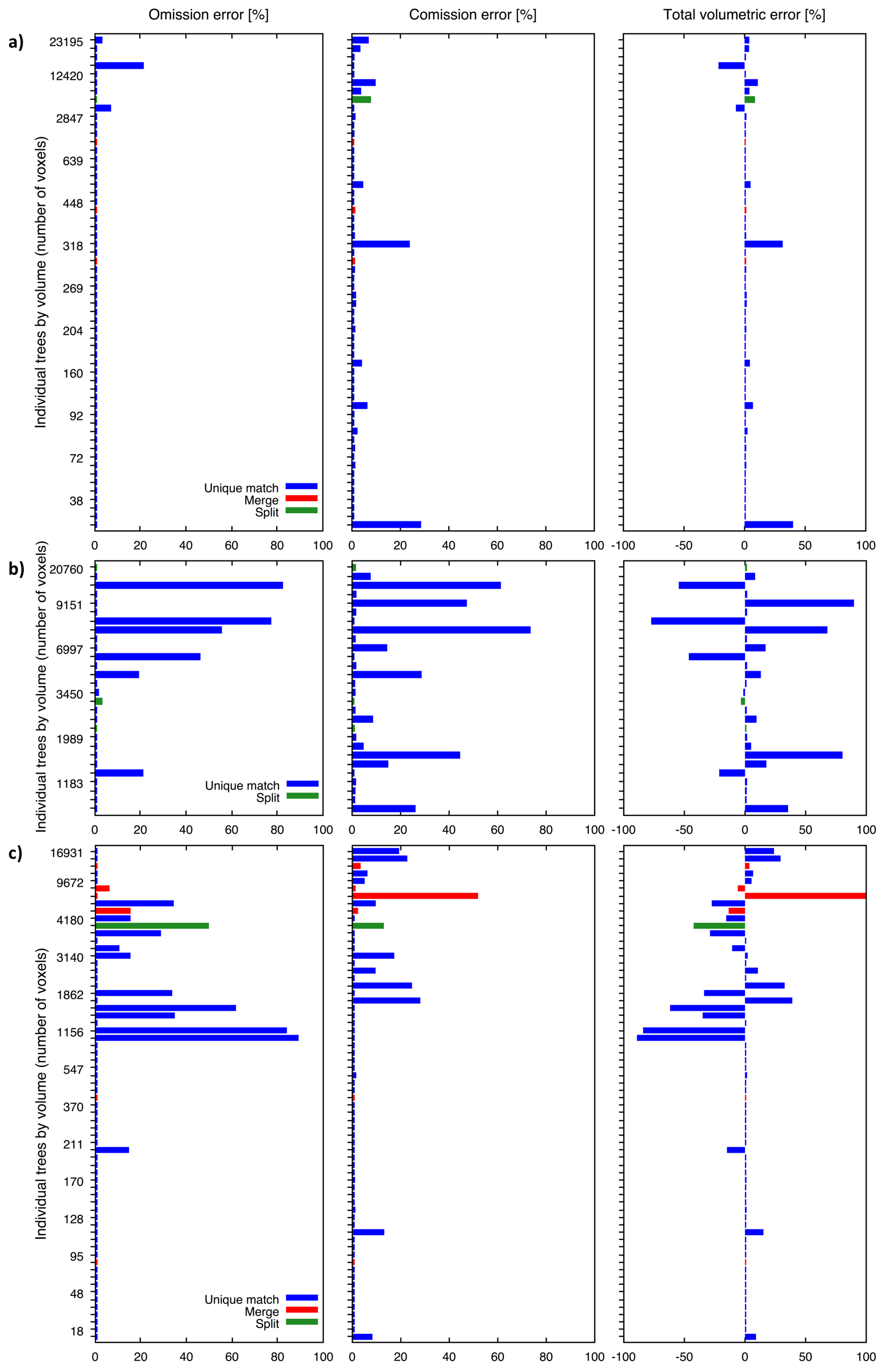
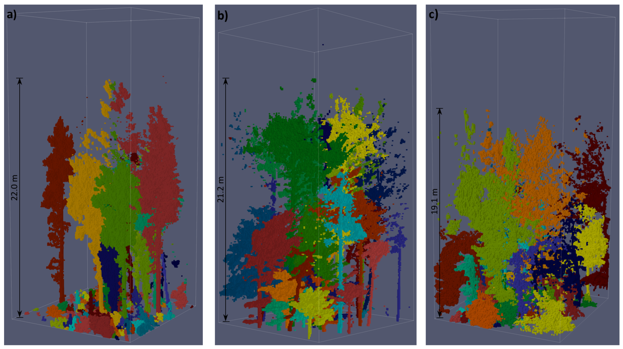
The validation results for the 3D shape and the volumetric match of the tree clusters are presented in Figure 4 and Table 3. Additionally, a visualization of the final tree clusters is given for the three reference quadrants in Figure 5. Parts (a) to (c) of Figure 4 also refer to these reference quadrants and provide detailed error information. The columns in each part of the figure separately list the omission error, the commission error and the total volumetric error. The omission error refers to the volume of intersection between the detected tree and its reference, divided by the total volume of the reference. The commission error is computed from the volume of intersection, compared to the total volume of the detected tree. The total volumetric error directly refers to the detected volume versus the reference volume, without considering any intersection. The error is given as percentage on the x-axis and the volume of the individual trees is given as number of voxels in sorted order on the y-axis. A blue coloured error bar indicates a unique allocation of a single cluster to a single reference, a red colour indicates a merge error and a green colour a split error.
Table 3 summarizes the accuracies for each reference quadrant. The average producer’s accuracy over all three plots amounted 93.66%, but reduced to 73.28% when only counting incorrect trees. The user’s accuracy was 94.06% for all trees and reduced to 89.53% for incorrect clusters.
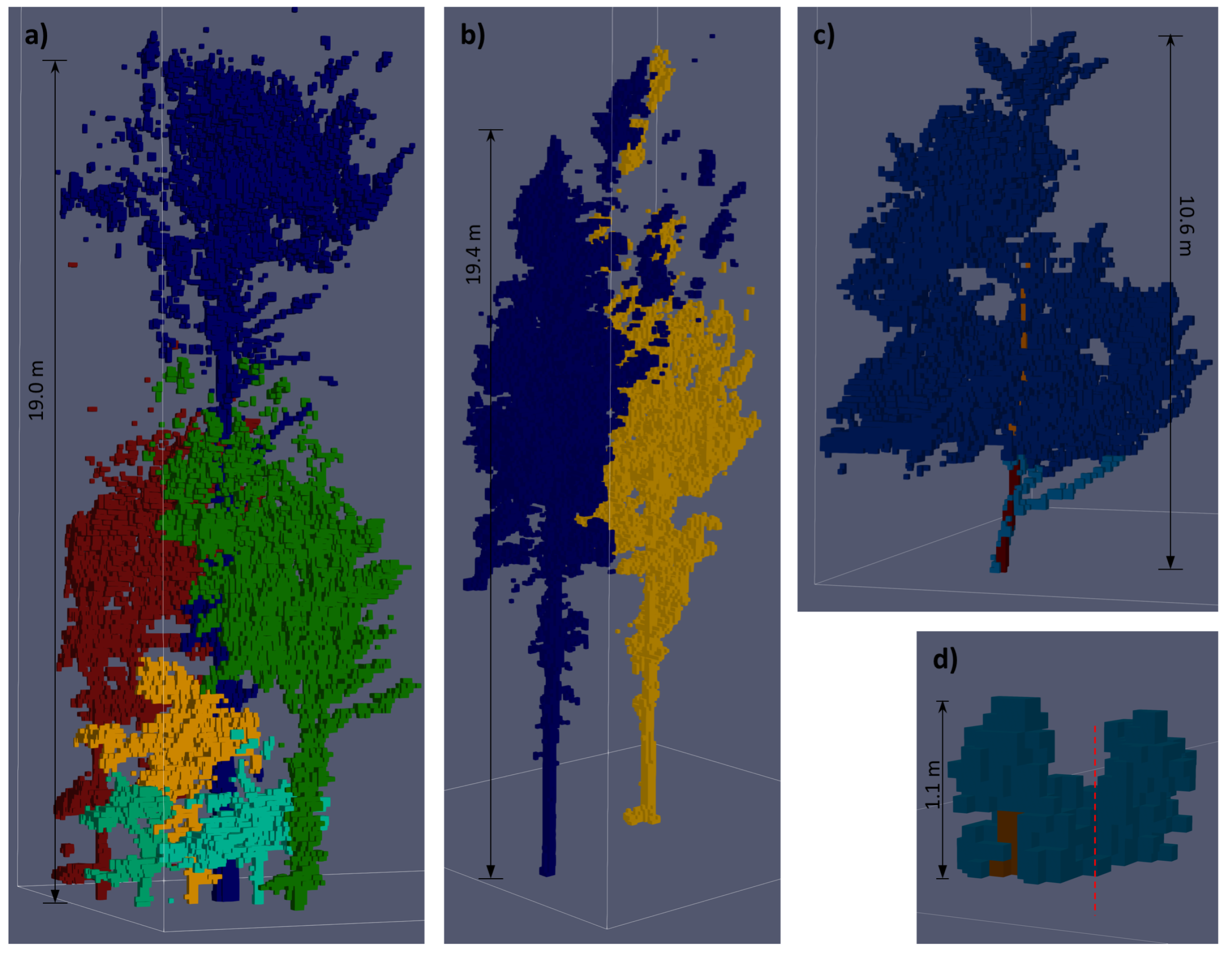
As addition to the numerical assessment, Figure 6 illustrates specific examples of the segmentation results. Part (a) provides an example for a vertically layered group of trees, with well isolated neighbouring trees of different sizes. Image (b) shows two mature trees that are well separated in the lower and middle parts but contain erroneous fragmentation in the upper part. Finally, images (c) and (d) give examples for splitting and merging errors. The split error in image (c) separates the lower tree stem and the tree crown in two clusters (different tones of blue). This is caused by erroneous separation of the related tree stem prior into two parts, which are indicted with different tones of brown. The merge error in image (d) shows a small tree cluster of low height, where only one stem was detected, but clear visual separation into two trees can be performed.

5. Discussion

The present study successfully combined state-of-the-art techniques for image analysis into an integrated workflow for single tree isolation. The method is able to handle difficult and dense forest data from TLS, which was a research gap until now. In technical comparison to many ALS based studies, the TLS data set is characterized by higher data density and by its perspective focus on understory and mid-layer trees. Together with the close to nature and dense forest stands, this was a challenging setting.

5.1. Methodical Approach

The individual techniques used in the overall framework had to be adapted and improved for the specific requirements of this application. For the detection of 3D tree stems, we rely on the previously published method of Heinzel and Huber [45]. This method could be directly applied without changes. Concerning the design of the distance parameters and the construction of the similarity graph, Reitberger et al. [21] provided specific ideas for the tree detection problem. We adapted and improved their ALS based approaches in order to model the similarities between image elements and to build the weight matrix. The TLS data concept required modification for much higher data density and the incorporation of advanced 3D stem information. In addition, other authors discussed similar types of distance parameter selection before. We can confirm the observations of Kamvar et al. [48], that the sensitivity parameters σ , for scaling the distance metrics in Equation (5), were critical factors for good segmentation results. The integration of prior information into spectral clustering was required to handle the dense forest and difficult forest structures. In this context we relied on the techniques described by Hu et al. [38], who presented an advanced and effective solution. Since their original method was designed for 2D colour images, it required adaption to 3D binary imagery. The final labelling problem could be solved by a MRF framework, as it was described by Komodakis and Tziritas [47] and Komodakis et al. [49]. We used the software implementation of the same authors, which produced adapted clusters for varying tree sizes. This avoided too balanced cluster sizes that are typical for spectral clustering, as explained by Von Luxburg [35]. The fact that the same MRF based labelling solution was also used by Hu et al. [38] allowed seamless integration in our overall method.

5.2. Interpretation of the Results

The combination of these single components was required, since attempts with reduced and simplified workflows were not successful. While Reitberger et al. [21] and Hu et al. [11] reported good results with less complex graph based clustering methods, we conclude that this is due to the use of ALS data and less dense forest stands, specifically in the understory. The validation results underline the success and capability of our approach to isolate single tree clusters for difficult and demanding settings. However, the details of the accuracy and error metrics must be interpreted correctly and the transferability to other forest types and wide area data was not tested in the framework of this methodical study.
Regarding the detection rate of correctly identified trees, almost all mature inventory trees with a DBH > 12 cm were detected correctly on all plots. As it can be seen from Table 2, only three errors occurred, which are due to combined stems of very close standing inventory trees. The increased stem diameter between the inner and the outer circle of the inventory system did not have any influence on the detection rate. However, the detection rate decreased for the regeneration trees with a DBH < 12 cm and amounted 84.62%. Even if this is still a good percentage, it indicates the increased difficulty of detecting small and often dense standing understory trees. This is mostly caused by the fact that the stems of small trees are often less visible in the data due to size and occlusion.
In addition to the pure detection rate, we verified the 3D extent and the volumetric match of the isolated trees without any restriction to stem diameter. This validation required extensive manual delineation of 3D references, which were compared to the detected tree clusters by an automated algorithm. The results for the first reference quadrant (Q1 in plot one) are presented in parts (a) of Figure 4 and Figure 5. Compared to the other reference quadrants, it is notable that the trees in this plot had the smallest errors. Furthermore, the forest structure was characterized by a large number of very small trees with heights below 130 cm, almost no intermediate layer and a few mature trees. Combining this information, it can be seen that the very small regeneration trees especially had noticeably small errors. In several cases, this is caused by visually inseparable natural clusters of these small trees that had to be used as references themselves. Interestingly, Reitberger et al. [21] reported similar problems even with larger understory trees. For future studies, a separate treatment of such very small trees might solve these problems. Despite the difficulties, Table 3 also shows that, when only considering erroneous tree clusters, the volumetric accuracies were still higher than 89%.
The results of the second reference quadrant (Q1 in plot four) are presented in part (b) of Figure 4 and Figure 5. The forest structure was distinguished from the first plot, since no layer of very small trees existed. It was characterized by mid and upper layers of dense and interlocked crown structure, but at least the lower parts of the stems were well visible. The major errors of this quadrant occurred in the upper canopy layer. They were caused by local problems of the interlocking crowns, but also due to a general problem of the terrestrial scanner perspective. The upper layer could be reached less well by the laser beam, so that the scan points strongly thinned out. This is the opposite effect as for airborne LiDAR systems. The low data density produced crown fragments in the upper layers, which were prone to misclassification. Image (b) in Figure 6 illustrates an example for such situation. Similarly, fragments from trees with stems outside the image, if not removed by postprocessing, were incorrectly allocated to clusters. These types of volumetric errors occurred despite the good detection rates of the trees themselves. However, visually, volumetric errors are often less noticeable because of their concentration in upper crown parts and border effects.
The third reference quadrant (Q1 in plot five) structurally distinguished from the other quadrants, since it had trees in all layers, including very small trees. Several beech trees and other deciduous trees were of irregular shapes and had interlocking tree crowns. From Table 3, it can be seen that the producer’s and user’s accuracy for erroneous tree clusters were similar to the accuracies of the second reference quadrant. In contrast, the accuracy calculated from all clusters is significantly higher on this quadrant. From the distribution of error in relation to tree volume, as apparent in Figure 4c, it can be inferred that this was caused by the existence of many very small trees. They had a similar positive effect on the overall accuracies like in the first reference quadrant.
Merging and splitting errors only played a minor role in the error statistics. The examples in Figure 6c,d demonstrate that such errors were caused by incorrect or missing stem priors. A strength of the present method was the good separation of vertically layered trees of different sizes. Figure 6a gives an example for such constellation, which typically is challenging for tree segmentation [21,22].

5.3. Comparison to Other Studies

The reported validation results are difficult to compare to other studies since only very few studies exist for tree segmentation from TLS forest data. Raumonen et al. [10] and Zhong et al. [30] are among the only authors. However, Raumonen et al. [10] did not provide accuracy metrics for the segmentation and used single trees segmentation in simple forest stands as pre-clustering stage for subsequent tree modelling. The good detection rates of Zhong et al. [30] of more than 90% are difficult to compare and interpret, since the authors sparsely described forest characteristics of their test sites and omitted a description of the reference data. Since they explained that their algorithm does not work in vertically structured forests and because they partly used MLS data close to urban locations, it can be assumed that their accuracies related to single layered and relatively simple forest structure or even urban trees. Validation results concerning the 3D shape of trees, are not available for TLS or ALS based studies. As a compromise, to give at least an impression on how our approach relates to other studies, we compared our positional tree detection rates with results from ALS based graph clustering approaches and from TLS based stem detection or positional tree detection methods.
For ALS based graph clustering, Reitberger et al. [21] achieved an overall tree detection rate of 59%, averaged over two main test sites with full-waveform data and using the best version of their algorithm. For trees in the upper layer, they reported a much higher rate of 86.5%, but, in the lower layer, it was only 19.0%. Strimbu and Strimbu [3] also used a graph based approach, but the clustering method was different. When omitting their results for plantation forest, the average detection rate was 92.71% for the upper layer, 75% for the intermediate layer and lower layer trees almost did not exist. Hu et al. [11] and Lee et al. [37] used graph clustering approaches as an intermediate step for tree modelling and tree species classification, and, therefore, they do not provide any assessment of the tree segmentation itself. Compared to our results, we achieved higher detection rates for both mature and regeneration trees. Especially for regeneration trees, the improvement was strongest, considering that Reitberger et al. [21] limited their reference trees to a relatively large minimum DBH of 10 cm. However, low detection rates for understory trees are typical for airborne data, since the number of reflections decreases while penetrating the canopy. Therefore, it is not necessarily a drawback of the ALS based algorithms, but reflects the difficulties our method has to deal with.
Despite the fact that several studies on stem detection from TLS data exist, only a few provided validation data that allowed for comparison to our study. Xia et al. [28] used TLS data from heterogeneous forests, but the average detection rate of 86% only considered non-occluded trees that were visible from a single-scan perspective. Brolly et al. [51] used data from a regeneration forest that did not cover mixed stands with different layers. They reported detection rates of 79% and 90%, but it remains unclear if they used data from a non-foliated state. Liang and Hyyppä [52] achieved an overall detection rate of 95.3%. Their test data was located in managed boreal forest, which is, even if dense by number of trees, typically less complexly structured and species-rich than our close to nature temperate forest. Furthermore, Rutzinger et al. [32] provided detection rates for mobile laser scanning data, but their study covered urban trees outside a forest environment and the verification method was missing. They reported percentages of 85% and 78% for two different test sites, of which the latter was described to contain a larger variety of tree sizes. In comparison to all these studies, our positional accuracies were at least similar for the regeneration trees and better for mature trees. It has to be considered that the other methods do not allow isolation of the complete trees including the tree crowns. Together with the complexity of our test data, this reveals a clear benefit of the new method.

6. Conclusions

We introduced a new approach for individual tree segmentation from high resolution TLS data. The method was developed and tested on nine sites with dense and complexly structured close to nature forest. Until now, TLS based single tree isolation and similarly difficult forest structures in general were only covered a little in literature. To handle this challenging task, semi-supervised learning with automatically extracted priors was applied for 3D image segmentation. Since most other tree detection approaches are based on ALS data, the presented method fills the gap of high resolution tree detection in the lower and intermediate forest layers. The new method was validated with a detailed assessment of the 3D tree shapes in addition to the tree positions. The overall good performance makes it interesting for applications in forest inventory and ecological studies, but wide area applications and other forest types need to be tested before. Future improvements could concentrate on eliminating border effects that result from trees whose stems are completely outside the image. An interesting option would also be to combine the TLS data with airborne data, which could possibly improve the information density in the upper canopy.

Author Contributions

J.H. conceived and developed the method, designed the fieldwork, and collected and processed the data. M.O.H. conceived and defined the main research objectives, designed the fieldwork, and managed the project. The manuscript was written by J.H. with input from M.O.H.

Funding

This study was conducted within the framework of the Swiss National Forest Inventory, a joint research program of the Swiss Federal Office for the Environment (FOEN) and the Swiss Federal Institute for Forest, Snow and Landscape Research (WSL). No further external funding was received.

Acknowledgments

The authors would like to thank Björn Dreier and Natalia Rehush for their support during the fieldwork, Christian Ginzler for his expertise in GNSS technology and Susette Haegi for registration of the scans. Special thanks go to the forest administration of the canton Grisons, Switzerland, who gave important assistance to this project.

Conflicts of Interest

The authors declare no conflict of interest.

References

  1. Pinz, A.J. Final results of the vision expert system VES: Finding trees in aerial photographs. In Wissensbasierte Mustererkennung; OCG Schriftenreihe; Institut für Elektrische Messtechnik Und Messsignalverarbeitung: Graz, Austria, 1989; Volume 49, pp. 90–111. [Google Scholar]
  2. Reitberger, J.; Schnörr, C.; Krzystek, P.; Stilla, U. 3D segmentation of full waveform LIDAR data for single tree detection using normalized cut. Int. Arch. Photogramm. Remote Sens. Spat. Inf. Sci. 2008, 37, 77–83. [Google Scholar]
  3. Strîmbu, V.F.; Strîmbu, B.M. A graph-based segmentation algorithm for tree crown extraction using airborne LiDAR data. ISPRS J. Photogramm. Remote Sens. 2015, 104, 30–43. [Google Scholar] [CrossRef]
  4. Mongus, D.; Žalik, B. An efficient approach to 3D single tree-crown delineation in LiDAR data. ISPRS J. Photogramm. Remote Sens. 2015, 108, 219–233. [Google Scholar] [CrossRef]
  5. Heinzel, J.N.; Weinacker, H.; Koch, B. Prior-knowledge-based single-tree extraction. Int. J. Remote Sens. 2011, 32, 4999–5020. [Google Scholar] [CrossRef]
  6. Leckie, D.; Gougeon, F.; Hill, D.; Quinn, R.; Armstrong, L.; Shreenan, R. Combined high-density lidar and multispectral imagery for individual tree crown analysis. Can. J. Remote Sens. 2003, 29, 633–649. [Google Scholar] [CrossRef] [Green Version]
  7. Hackenberg, J.; Morhart, C.; Sheppard, J.; Spiecker, H.; Disney, M. Highly Accurate Tree Models Derived from Terrestrial Laser Scan Data: A Method Description. Forests 2014, 5, 1069–1105. [Google Scholar] [CrossRef] [Green Version]
  8. Raumonen, P.; Kaasalainen, M.; Åkerblom, M.; Kaasalainen, S.; Kaartinen, H.; Vastaranta, M.; Holopainen, M.; Disney, M.; Lewis, P. Fast Automatic Precision Tree Models from Terrestrial Laser Scanner Data. Remote Sens. 2013, 5, 491–520. [Google Scholar] [CrossRef] [Green Version]
  9. Hosoi, F.; Nakai, Y.; Omasa, K. 3-D voxel-based solid modeling of a broad-leaved tree for accurate volume estimation using portable scanning lidar. ISPRS J. Photogramm. Remote Sens. 2013, 82, 41–48. [Google Scholar] [CrossRef]
  10. Raumonen, P.; Casella, E.; Calders, K.; Murphy, S.; Åkerbloma, M.; Kaasalainen, M. Massive-scale tree modelling from TLS data. ISPRS Ann. Photogramm. Remote Sens. Spat. Inf. Sci. 2015, II-3/W4, 189–196. [Google Scholar] [CrossRef]
  11. Hu, S.; Li, Z.; Zhang, Z.; He, D.; Wimmer, M. Efficient tree modeling from airborne LiDAR point clouds. Comput. Graph. 2017, 67, 1–13. [Google Scholar] [CrossRef]
  12. Calders, K.; Newnham, G.; Burt, A.; Murphy, S.; Raumonen, P.; Herold, M.; Culvenor, D.; Avitabile, V.; Disney, M.; Armston, J.; et al. Nondestructive estimates of above-ground biomass using terrestrial laser scanning. Methods Ecol. Evol. 2014, 6, 198–208. [Google Scholar] [CrossRef] [Green Version]
  13. Kaartinen, H.; Hyyppä, J.; Yu, X.; Vastaranta, M.; Hyyppä, H.; Kukko, A.; Holopainen, M.; Heipke, C.; Hirschmugl, M.; Morsdorf, F.; et al. An International Comparison of Individual Tree Detection and Extraction Using Airborne Laser Scanning. Remote Sens. 2012, 4, 950–974. [Google Scholar] [CrossRef] [Green Version]
  14. Menk, J.; Dorren, L.; Heinzel, J.; Marty, M.; Huber, M. Evaluation automatischer Einzelbaumerkennung aus luftgestützten Laserscanning-Daten. Schweizerische Zeitschrift fur Forstwesen 2017, 168, 151–159. [Google Scholar] [CrossRef]
  15. Kwak, D.A.; Lee, W.K.; Lee, J.H.; Biging, G.S.; Gong, P. Detection of individual trees and estimation of tree height using LiDAR data. J. For. Res. 2007, 12, 425–434. [Google Scholar] [CrossRef]
  16. Baumann, A.B.G.; Baltsavias, E. Einzelbaumdetektion in bewaldetem Gebiet auf Basis von luftgestützten LiDAR-Daten. In Proceedings of the Dreiländertagung der DGPF, der OVG und der SGPF, Bern, Schweiz, 6–9 June 2016; Kersten, T.P., Ed.; Volume 25, pp. 506–515. [Google Scholar]
  17. Chmielewski, L.J.; Bator, M.; Zasada, M.; Stereńczak, K.; Strzeliński, P. Fuzzy Hough Transform-Based Methods for Extraction and Measurements of Single Trees in Large-Volume 3D Terrestrial LIDAR Data. In Computer Vision and Graphics; Springer: Berlin/Heidelberg, Germany, 2010; pp. 265–274. [Google Scholar]
  18. Bienert, A.; Scheller, S.; Keane, E.; Mohan, F.; Nugent, C. Tree detection and diameter estimations by analysis of forest terrestrial laserscanner point clouds. Int. Arch. Photogramm. Remote Sens. Spat. Inf. Sci. 2007, XXXVI-3/W52, 50–55. [Google Scholar]
  19. Lee, H.; Slatton, K.C.; Roth, B.E.; Cropper, W.P. Adaptive clustering of airborne LiDAR data to segment individual tree crowns in managed pine forests. Int. J. Remote Sens. 2010, 31, 117–139. [Google Scholar] [CrossRef]
  20. Bienert, A.; Queck, R.; Schmidt, A.; Bernhofer, C.; Maas, H. Voxel space analysis of terrestrial laser scans in forests for wind field modelling. Int. Arch. Photogramm. Remote Sens. Spat. Inf. Sci. 2010, 38, 92–97. [Google Scholar]
  21. Reitberger, J.; Schnörr, C.; Krzystek, P.; Stilla, U. 3D segmentation of single trees exploiting full waveform LIDAR data. ISPRS J. Photogramm. Remote Sens. 2009, 64, 561–574. [Google Scholar] [CrossRef]
  22. Duncanson, L.; Cook, B.; Hurtt, G.; Dubayah, R. An efficient, multi-layered crown delineation algorithm for mapping individual tree structure across multiple ecosystems. Remote Sens. Environ. 2014, 154, 378–386. [Google Scholar] [CrossRef]
  23. Wang, Y.; Hyyppa, J.; Liang, X.; Kaartinen, H.; Yu, X.; Lindberg, E.; Holmgren, J.; Qin, Y.; Mallet, C.; Ferraz, A.; et al. International Benchmarking of the Individual Tree Detection Methods for Modeling 3-D Canopy Structure for Silviculture and Forest Ecology Using Airborne Laser Scanning. IEEE Trans. Geosci. Remote Sens. 2016, 54, 5011–5027. [Google Scholar] [CrossRef]
  24. Li, W.; Guo, Q.; Jakubowski, M.K.; Kelly, M. A new method for segmenting individual trees from the lidar point cloud. Photogramm. Eng. Remote Sens. 2012, 78, 75–84. [Google Scholar] [CrossRef]
  25. Lu, X.; Guo, Q.; Li, W.; Flanagan, J. A bottom-up approach to segment individual deciduous trees using leaf-off lidar point cloud data. ISPRS J. Photogramm. Remote Sens. 2014, 94, 1–12. [Google Scholar] [CrossRef]
  26. Heurich, M.; Persson, Å.; Holmgren, J.; Kennel, E. Detecting and measuring individual trees with laser scanning in mixed mountain forest of central Europe using an algorithm developed for Swedish boreal forest conditions. Int. Arch. Photogramm. Remote Sens. Spat. Inf. Sci. 2004, 36, 307–312. [Google Scholar]
  27. Weinacker, H.; Koch, B.; Heyder, U.; Weinacker, R. Development of filtering, segmentation and modelling modules for lidar and multispectral data as a fundament of an automatic forest inventory system. Int. Arch. Photogramm. Remote Sens. Spat. Inf. Sci. 2004, 36, W2. [Google Scholar]
  28. Xia, S.; Wang, C.; Pan, F.; Xi, X.; Zeng, H.; Liu, H. Detecting stems in dense and homogeneous forest using single-scan TLS. Forests 2015, 6, 3923–3945. [Google Scholar] [CrossRef]
  29. Bienert, A.; Schneider, D. Range image segmentation for tree detection in forest scans. Int. Arch. Photogramm. Remote Sens. Spat. Inf. Sci. 2013, II-5/W2, 49–54. [Google Scholar] [CrossRef]
  30. Zhong, L.; Cheng, L.; Xu, H.; Wu, Y.; Chen, Y.; Li, M. Segmentation of Individual Trees From TLS and MLS Data. IEEE J. Sel. Top. Appl. Earth Obs. Remote Sens. 2017, 10, 774–787. [Google Scholar] [CrossRef]
  31. Zou, X.; Cheng, M.; Wang, C.; Xia, Y.; Li, J. Tree Classification in Complex Forest Point Clouds Based on Deep Learning. IEEE Geosci. Remote Sens. Lett. 2017, 14, 2360–2364. [Google Scholar] [CrossRef]
  32. Rutzinger, M.; Pratihast, A.; Oude Elberink, S.; Vosselman, G. Detection and modelling of 3D trees from mobile laser scanning data. Int. Arch. Photogramm. Remote Sens. Spat. Inf. Sci. 2010, 38, 520–525. [Google Scholar]
  33. Lin, Y.; Hyyppä, J.; Jaakkola, A.; Yu, X. Three-level frame and RD-schematic algorithm for automatic detection of individual trees from MLS point clouds. Int. J. Remote Sens. 2012, 33, 1701–1716. [Google Scholar] [CrossRef]
  34. Wu, B.; Yu, B.; Yue, W.; Shu, S.; Tan, W.; Hu, C.; Huang, Y.; Wu, J.; Liu, H. A Voxel-Based Method for Automated Identification and Morphological Parameters Estimation of Individual Street Trees from Mobile Laser Scanning Data. Remote Sens. 2013, 5, 584–611. [Google Scholar] [CrossRef] [Green Version]
  35. Von Luxburg, U. A tutorial on spectral clustering. Stat. Comput. 2007, 17, 395–416. [Google Scholar] [CrossRef] [Green Version]
  36. Shi, J.; Malik, J. Normalized cuts and image segmentation. IEEE Trans. Pattern Anal. Mach. Intell. 2000, 22, 888–905. [Google Scholar] [Green Version]
  37. Lee, J.; Cai, X.; Lellmann, J.; Dalponte, M.; Malhi, Y.; Butt, N.; Morecroft, M.; Schonlieb, C.B.; Coomes, D.A. Individual Tree Species Classification From Airborne Multisensor Imagery Using Robust PCA. IEEE J. Sel. Top. Appl. Earth Obs. Remote Sens. 2016, 9, 2554–2567. [Google Scholar] [CrossRef]
  38. Hu, H.; Feng, J.; Yu, C.; Zhou, J. Multi-class constrained normalized cut with hard, soft, unary and pairwise priors and its applications to object segmentation. IEEE Trans. Image Process. 2013, 22, 4328–4340. [Google Scholar] [CrossRef] [PubMed]
  39. Klein, D.; Kamvar, S.D.; Manning, C.D. From instance-level constraints to space-level constraints: Making the most of prior knowledge in data clustering. In Proceedings of the Nineteenth International Conference on Machine Learning, Sydney, Australia, 8–12 July 2002; pp. 307–314. [Google Scholar]
  40. Peluffo-Ordóñez, D.H.; Castro-Ospina, A.E.; Chavez-Chamorro, D.; Acosta-Medina, C.D.; Castellanos-Domínguez, G. Normalized cuts clustering with prior knowledge and a pre-clustering stage. In Proceedings of the European Symposium on Artificial Neural Networks, Bruges, Belgium, 24–26 April 2013; pp. 309–314. [Google Scholar]
  41. Yao, T.; Yang, X.; Zhao, F.; Wang, Z.; Zhang, Q.; Jupp, D.; Lovell, J.; Culvenor, D.; Newnham, G.; Ni-Meister, W.; et al. Measuring forest structure and biomass in New England forest stands using Echidna ground-based lidar. Remote Sens. Environ. 2011, 115, 2965–2974. [Google Scholar] [CrossRef]
  42. Zande, D.V.d.; Jonckheere, I.; Stuckens, J.; Verstraeten, W.W.; Coppin, P. Sampling design of ground-based lidar measurements of forest canopy structure and its effect on shadowing. Can. J. Remote Sens. 2008, 34, 526–538. [Google Scholar] [CrossRef]
  43. FARO Technologies Inc. FARO SCENE 5.1 Users Manual; FARO: Lake Mary, FL, USA, 2014. [Google Scholar]
  44. Ayachit, U. The ParaView Guide; Kitware Inc.: New York, NY, USA, 2016; p. 237. [Google Scholar]
  45. Heinzel, J.; Huber, M. Detecting Tree Stems from Volumetric TLS Data in Forest Environments with Rich Understory. Remote Sens. 2017, 9, 9. [Google Scholar] [CrossRef]
  46. Soille, P. Morphological Image Analysis: Principles and Applications; Springer: Berlin/Heidelberg, Germany; New York, NY, USA, 2004; p. 302. [Google Scholar]
  47. Komodakis, N.; Tziritas, G. Approximate Labeling via Graph Cuts Based on Linear Programming. IEEE Trans. Pattern Anal. Mach. Intell. 2007, 29, 1436–1453. [Google Scholar] [CrossRef] [PubMed]
  48. Kamvar, K.; Sepandar, S.; Klein, K.; Dan, D.; Manning, M.; Christopher, C. Spectral learning. In Proceedings of the International Joint Conference of Artificial Intelligence, Acapulco, Mexico, 9–15 August 2003. [Google Scholar]
  49. Komodakis, N.; Tziritas, G.; Paragios, N. Performance vs computational efficiency for optimizing single and dynamic MRFs: Setting the state of the art with primal-dual strategies. Comput. Vis. Image Underst. 2008, 112, 14–29. [Google Scholar] [CrossRef] [Green Version]
  50. Congalton, R.G. A review of assessing the accuracy of classifications of remotely sensed data. Remote Sens. Environ. 1991, 37, 35–46. [Google Scholar] [CrossRef]
  51. Brolly, G.; Király, G.; Czimber, K. Mapping Forest Regeneration from Terrestrial Laser Scans. Acta Silv. Lign. Hung. 2013, 9, 135–146. [Google Scholar] [CrossRef] [Green Version]
  52. Liang, X.; Hyyppä, J. Automatic Stem Mapping by Merging Several Terrestrial Laser Scans at the Feature and Decision Levels. Sensors 2013, 13, 1614–1634. [Google Scholar] [CrossRef] [PubMed] [Green Version]
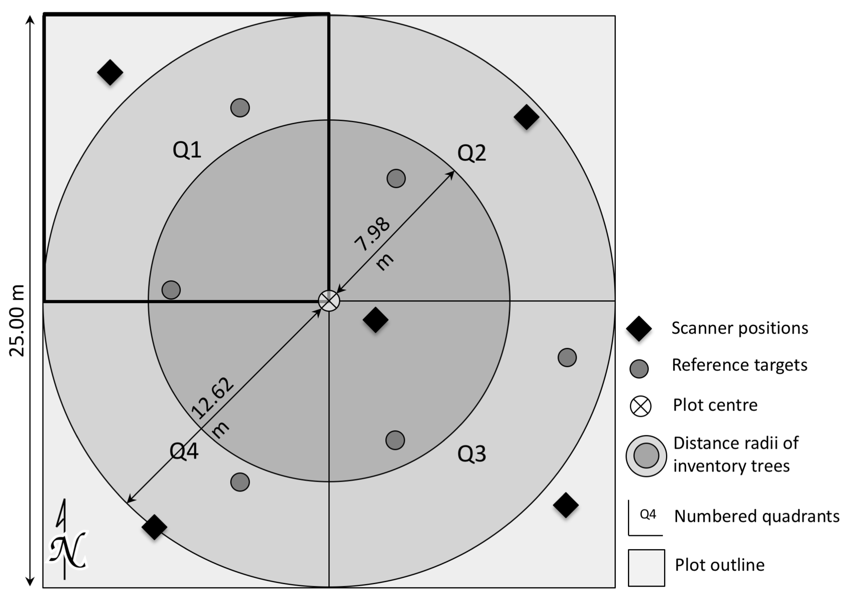
Figure 1. Schematic composition of a sample plot for terrestrial laser scanning and reference data collection. The square shaped plots had an edge length of 25 m and were centred on the original inventory points. The two concentric circles indicate the distances for mature tree data collection by the forest inventory. The plots were split into four quadrants for processing, whereof the first quadrants (Q1) were used for 3D validation (marked with bold outline). Scanner positions and reference targets were distributed over the plot to minimize occlusion effects.
Remotesensing 10 01056 g001
Figure 2. Illustration of the overall workflow for single tree segmentation. For the main steps, intermediate results are visualized by using a plot quadrant as example. (a) shows the initial point cloud overlaid with red-green-blue (RGB) photographs for visual appearance; (b) depicts the vegetation voxel grid after preprocessing; (c) illustrates the isolated tree stems. The vegetation image and the tree stems were used to build the similarity graph in (d). Afterwards, the eigenspectrum of the graph was computed and weighted using stem information; (e) visualizes single vectors of the spectrum as image stack; (f) shows the tree clusters after labelling in a Markov Random Field (MRF) framework. Final results after postprocessing are illustrated in (g).
Remotesensing 10 01056 g002
Figure 3. Flowchart providing an overview on the single steps of constrained spectral clustering. The three main steps that are described in Section 3.3.1, Section 3.3.2 and Section 3.3.3 are grouped with braces.
Remotesensing 10 01056 g003
Figure 4. Error metrics referring to the intersection and volumetric match between the detected tree clusters and the manually digitized 3D references. (ac) show the results for the first quadrants of plots one, four and five, respectively. For each plot, the omission, commission and the total volumetric error are given as percentage on the x-axes. The volume is indicated as number of voxels for the individual trees on the y-axes and sorted in decreasing order. Additionally, merge and split errors are indicated by the colour of the error bar.
Remotesensing 10 01056 g004
Figure 5. Final clustering results of the quadrants Q1 on plots one, four and five. Plot one in (a) is characterized by many small trees close to the ground and grouped trees in the upper layer. Plot four in (b) has an interlocking crown structure in the mid and upper layers with clearly visible stems below. Plot five in (c) has trees in all layers, is densely structured and has crowns of irregular shape.
Remotesensing 10 01056 g005
Figure 6. Examples of isolated trees. (a) shows a group of well isolated trees in a vertically structured composition; (b) gives an example of major trees with isolated fragments at the crown top and at the image border; (c) shows a splitting error, where the lower stem part and the crown were separated into two clusters (tones of blue) due to erroneously split stem priors (tones of brown); (d) is an example for a merge error of a very small tree cluster. The cluster is clearly separable into two trees (red line), but only one stem prior is existing (brown colour).
Remotesensing 10 01056 g006
Table 1. Overview of the sample plot characteristics. The table lists forest type and structural forest information, which are critical factors for single tree segmentation.
Plot №Forest Type and SpeciesNumber of Mature TreesRegeneration Canopy CoverageGeneral Description of Layers and Structure
Tree Height 1.3 mTree Height  > 1.3 m and DBH ≤ 12 cm
1Mixed (fir, pine, spruce, beech)7 DBH 12–36 cm
4 DBH > 36 cm
Fir 6–15%Fir 16–25%
Spruce 6–15%
Beech 6–15%
Lower and upper layer predominant. Lower layer contains small trees in dense and patchy clusters (height < 130 cm).
2Mixed (pine, spruce, beech, ash, elm)8 DBH 12–36 cm
9 DBH > 36 cm
Beech 16–25%
Others 6–15%
Beech 26–50%
Elm 6–15%
Lower layer dominated by very small trees (< 130 cm), mature trees of relatively low height (∼17 m).
3Mixed (pine, spruce, rowan, sorb, alder)9 DBH 12–36 cm
2 DBH > 36 cm
All spec. ≤ 5%Spruce 6–15%
Sorb 6–15%
Alder 6–15%
Mid layer interlocking with upper layer trees. Upper layer of relatively low height (∼16 m).
4Mixed (fir, pine, spruce, beech)10 DBH 12–36 cm
7 DBH > 36 cm
All spec. ≤ 5%Fir 16–25%
Spruce 26–50%
Beech 16–25%
Continuous height transition between mid and upper layers. Strongly interlocking crowns but good stem visibility.
5Mixed (pine, spruce, larch, beech, ash, maple)15 DBH 12–36 cm
3 DBH > 36 cm
Ash 51–75%
Maple 6–15%
Ash 6–15%
Beech 16–25%
All layers equally represented. Appears visually unstructured with strongly interlocking crowns.
6Mixed (pine, spruce, larch, beech, oak, poplar)6 DBH 12–36 cm
7 DBH > 36 cm
Beech 6–15%Beech 51–75%
Poplar 26–59%
Lower an mid layers predominant. Upper layer with irregular distribution of trees.
7Coniferous (spruce, larch), deciduous lower layer (rowan)9 DBH 12–36 cmAll spec. ≤ 5%Larch 6–15%Predominant upper layer with spruce mature trees. Sparse lower an mid layers.
8Coniferous (spruce), deciduous lower layer (rowan)3 DBH 12–36 cm
3 DBH > 36 cm
All spec. ≤ 5%Spruce 16–25%Equal ratio of lower, mid and upper layer trees. Clustered distribution.
9Coniferous (spruce), deciduous lower and mid layers (rowan)12 DBH > 36 cmRowan 16–25%Spruce 6–15%
Rowan 16–25%
Predominant upper and mid layers with spruce trees. Sparse lower layer.
Table 2. Rates for automatically detected trees (auto) compared to the references measured in the field (ref).
Plot №Mature TreesRegeneration Trees
DBH ≥ 12 cmDBH ≥ 36 cmDBH < 12 cm
Auto/RefAuto/RefAuto/Ref
17/74/48/9
210/116/61/2
310/101/10/1
413/134/46/7
515/153/33/5
610/103/39/12
74/53/44/4
84/42/29/10
92/210/1015/15
Rate [%]97.4097.3084.62
Table 3. Producer’s and user’s accuracies for 3D validation of tree segmentation. Both types of accuracies were calculated for all tree clusters of the plot quadrant and only for tree clusters with a volumetric error >0.
Q1 of Plot №Producer’s Accuracy [%]User’s Accuracy [%]
All ClustersIncorrect ClustersAll ClustersIncorrect Clusters
199.4589.3498.0695.51
489.0265.8487.7485.70
592.5064.6696.3787.39
Average93.6673.2894.0689.53