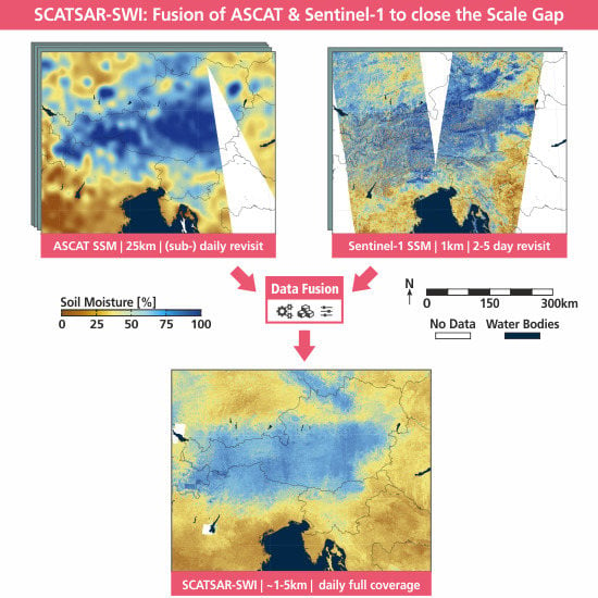
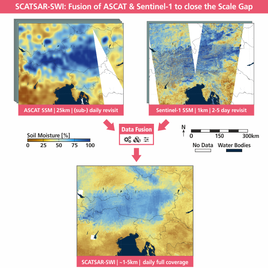
Soil Moisture from Fusion of Scatterometer and SAR: Closing the Scale Gap with Temporal Filtering

Abstract

Soil moisture is a key environmental variable, important to e.g., farmers, meteorologists, and disaster management units. We fuse surface soil moisture (SSM) estimates from spatio-temporally complementary radar sensors through temporal filtering of their joint signal and obtain a kilometre-scale, daily soil water content product named SCATSAR-SWI. With 25 km Metop ASCAT SSM and 1 km Sentinel-1 SSM serving as input, the SCATSAR-SWI is globally applicable and achieves daily full coverage over operated areas. We employ a near-real-time-capable SCATSAR-SWI algorithm on a fused 3 year ASCAT-Sentinel-1-SSM data cube over Italy, obtaining a consistent set of model parameters, unperturbed by coverage discontinuities. An evaluation of a therefrom generated SCATSAR-SWI dataset, involving a 1 km Soil Water Balance Model (SWBM) over Umbria, yields comprehensively high agreement with the reference data (median R = 0.61 vs. in situ; 0.71 vs. model; 0.83 vs. ASCAT SSM). While the Sentinel-1 signal is attenuated to some extent, the ASCAT’s signal dynamics are fully transferred to the SCATSAR-SWI and benefit from the Sentinel-1 parametrisation. Using the SM2RAIN approach, the SCATSAR-SWI shows excellent capability to reproduce 5 day-accumulated rainfall over Italy, with R = 0.89 against observed rainfall. The SCATSAR-SWI is currently in preparation towards operational product dissemination in the Copernicus Global Land Service (CGLS).

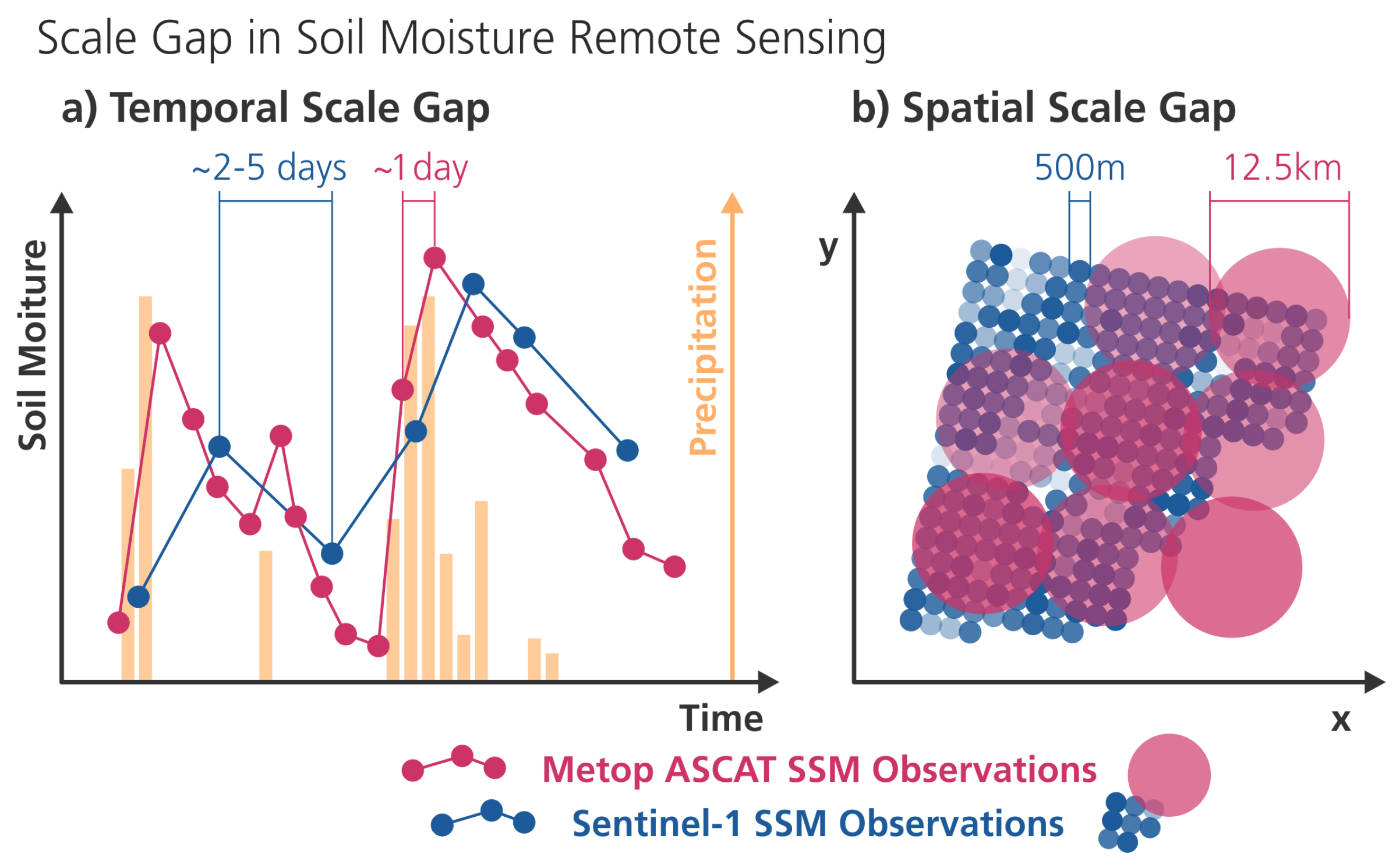
1. Introduction

Dynamics in soil moisture (SM) are important in the understanding of processes in many environmental and socio-economic fields, e.g., its impact on vegetation vitality, crop yield, droughts or exposure to flood threats. SM is a key driver of water and heat fluxes between the ground and the atmosphere, regulating air temperature and humidity [1]. Vice versa, Surface Soil Moisture (SSM), which is the water content in the soil’s top centimetres, is very sensitive to external forcing in the form of precipitation, temperature, solar irradiation, humidity, and wind. SM is thus both an integrator of climatic conditions [2] and a driver of local weather and climate [3], and plays a major role in global water-, energy- and carbon- cycles [4].

Consequently, knowledge of the spatial and temporal variation of SM is crucial to users in meteorology, climatology, hydrology, and agronomy. More specifically, estimation of SM can be a critical skill in numerical weather prediction [5,6,7], precipitation estimation [8,9], flood risk modelling [10,11], runoff prediction [12], groundwater recharge modelling [13], and irrigation assessment [14]. Furthermore, estimation of SM is crucial for creating understanding of heatwaves [15], droughts [16], ocean–land feedback [17], and long-term trends in hydrology [18]. On these grounds, soil moisture is listed as essential climate variable (ECV) within the framework of the Global Climate Observing System [19].

With increasing expectations towards these applications, the demand for observational data with high spatio-temporal resolution, as well as complete coverage, is steadily growing. While in situ techniques [20] allow for accurate and temporally dense measurements at point scale, they lack spatial representativeness and require equipment, maintenance and ground access, leaving many parts of the world unobserved. For extensive or global undertakings, Earth observation, and more specifically, spaceborne microwave remote sensing has proven its capability to retrieve soil moisture comprehensively. Satellites carrying microwave sensors record surface properties, globally and independently from daylight and cloud cover, and SM products therefrom reached maturity in the last decade [21]. Coarse-scale SM products (12–50 km) from active (radars) or passive sensors (radiometers) like SM from Metop ASCAT [22], Windsat [23], SMOS [24], and SMAP [25] have been thoroughly evaluated and have found widespread use [26,27]. These products have a large swath/footprint and can well capture temporal SM dynamics with their daily or sub-daily revisit times. However, they lack spatial details. They do not support analysis of local hydrological patterns below the 10 km scale, such as effects from convectional rains or topography and thus do not meet the requirements of many users.

On the other hand, Synthetic Aperture Radar (SAR) remote sensing systems like the (elapsed) Envisat ASAR and the current Sentinel-1 (S-1) CSAR radar provide sub-antenna footprint resolution through advanced radar signal processing, involving range and Doppler discrimination [28]. With this imaging technique, the sensors deliver high-resolution radar imagery of the ground’s geometric and dielectric properties, potentially resolving objects at the field level. Envisat ASAR was already successfully employed for SSM retrieval [29] during the period 2004–2012, showing capability to monitor soil moisture dynamics at the continental level and potential for model assimilation [30]. Recently, the approach was adapted to its successor SAR mission Sentinel-1 [31], aiming for global monitoring of SSM at the kilometre scale. However, SAR, and in general all high resolution systems, observe individual locations less frequently and thus often fail to capture short-term variations, like during rainfall events.

However, for a single remote sensing system, there always exists a trade-off between spatial and temporal resolution of the observations, leading to missed dynamics either in the spatial or temporal domain. We exemplify the scale gap in remote sensing with the illustration in Figure 1, sketching the characteristics of the SSM products from Metop ASCAT [22] and Sentinel-1 [31]. While the SAR product does not measure often enough to fully capture the SM variations induced by rainfall, the ASCAT product has a much coarser resolution.

With the aim to improve the spatial resolution of the short-repeating coarse-scale SM products, several approaches to estimate sub-pixel information can be found. These methods range from geostatistical analysis [32], downscaling algorithms applying subpixel-patterns [33,34,35], to multi-band products [36,37]. They have in common the need for apt auxiliary data, either temporally concurring observations from different bands, or a-priori local data as e.g., knowledge on the local land cover or soil properties, which are commonly neither available everywhere nor of consistent quality. A comprehensive survey on soil moisture downscaling methods is given, e.g., by [38].

In the present study, we suggest a data fusion approach in order to generate a high-resolution, high-frequency SSM product, taking up the concept of temporal stability of soil moisture [39]. The concept suggests that a local SM signal is highly correlated with the regional SM signal from its larger surrounding area. Hence, where this assumption holds true, a region’s individual zones are subject to persistent regional SM patterns and thus show similar soil moisture dynamics. In this case, a fusion of datasets that are recorded at different scales but describe SM in the same way is valid. In that sense, we identified SSM from scatterometers (coarse-scale) and SAR (fine-scale) as a suitable set of datasets for fusion.

In our method, the actual fusion of the SM signals is realised through temporal filtering at each gridded pixel, following the Soil Water Index (SWI) approach [40] that estimates the water content of soil profile layer $W_{PL}\left(t\right)$ from the local history of the surface layer’s water content $W_{SL}\left(\tau \right)$:

$$W_{PL}\left(t\right)={\displaystyle \frac{1}{T}}{\int }_t^{-\infty }{W}_{SL}\left(\tau \right)e^{\frac{-(t-\tau )}{T}}d\tau .$$

(1)

This approach represents a simple two-layer water balance model, consisting of a top layer ($SL$), which is accessible to C-band sensors, and the profile layer ($PL$), which extends downwards. The $PL$ is assumed to serve as a reservoir, connected to the atmosphere only via $SL$. The $SL$ is in direct contact with the atmosphere and its water content is thus temporally highly dynamic. For the underneath $PL$, the amount of stored water depends on the infiltration of water added to $SL$ during precipitation events. Hence, the SM in $PL$ can be solely explained by the past dynamics of $SL$, with more recent events having a stronger impact, which is accounted for by the exponential weighting function in Equation (1). Here, T is the so-called characteristic time length (the T-value) and acts as a local and soil-dependent measure for the infiltration time, hence increasing with depth of $PL$. Naturally, the temporal SM dynamics are decreasing with depth, as with increasing depth more antecedent SSM observations are effectively integrated. With remotely sensed $\mathrm{SSM}\left(t_i\right)$ as measurements of $W_{SL}$, the SWI is formulated by [40] accordingly as

$${\mathrm{SWI}}_T\left(t_n\right)=\frac{{{\displaystyle \sum }}_i^n\mathrm{SSM}\left(t_i\right)e^{-\frac{t_n-t_i}{T}}}{{{\displaystyle \sum }}_i^n{e}^{-\frac{t_n-t_i}{T}}}\mathrm{for}{t}_i\le t_n,$$

(2)

where $t_n$ is the observation time of the current SSM measurement and $t_i$ are the observations times of the previous SSM measurements. All SSM observations before $t_n$ are summed up and exponentially weighted and the T-value determines how fast the weights become smaller, thus modelling how strongly past SSM observations influence the SWI value. An examination of how the T-values correspond to soil depth can be found in [41].

The SWI formulation allows to propagate SSM values forward in time, modelling the infiltration into the soil’s deeper layers. When we now combine coexisting streams of SSM signals to a fused SSM-history $W_{SL}\left(\tau \right)$, we obtain, through the temporal filtering, a SWI value that carries the SM information from all the input streams. When we fuse SSM from SCAT and SAR systems, and when we do the SWI-filtering for each individual location of the SAR’s fine-scale grid, we may transfer the high spatial resolution of the SAR SSM, as well as the high temporal resolution of the SCAT SSM, to the SWI product.

Based on these considerations, we develop a near-real-time (NRT) capable data fusion algorithm to overcome the remote sensing scale gap, by ingesting two streams of radar observations from complementary spatio-temporal scale. Assuming that they describe soil moisture processes similarly, we merge coarse-scale SSM signals from Metop ASCAT (scatterometer, 25 km resolution) and fine-scale SSM signals from Sentinel-1 (SAR, 1 km), and yield a high-resolution, high-frequency soil water index product named Scatterometer Synthetic Aperture Radar Soil Water Index (SCATSAR-SWI). Benefiting from the input’s either high temporal or spatial resolution, respectively, this kilometre-scale daily product provides observational data for operational use, at full spatial extent each day.

In the following Section 2, we describe the input datasets of the SCATSAR-SWI in detail while Section 3 presents the algorithmic implementation of its retrieval. In Section 4, we explain the evaluation experiments and reference datasets, which is followed by the results and discussions in Section 5. The articles closes with general conclusions and an outlook in Section 6.

2. Input Datasets

The here presented SCATSAR-SWI fuses 25 km Metop ASCAT SSM and 1 km Sentinel-1 SSM data to one SWI dataset. Both input datasets are generated with an SSM retrieval method employing the TU Wien Change Detection Model [40], which derives SSM directly from observed radar backscatter, measured as backscatter coefficient ${\sigma }^0$. In this model, changes in backscatter are interpreted as changes in soil moisture while other surface properties, such as geometry, roughness, and vegetation type, are interpreted as static parameters. The parameters describe maximum dry- and wet- conditions as well as average vegetation and surface geometry signal contributions. The model is self-calibrated at the pixel scale as the model parameters are estimated through statistical analysis of long-term backscatter time series. The obtained SSM values represent the degree of saturation of the topmost soil layer (first ∼5 cm) and are given in relative units ranging from 0% (dry) to 100% (wet). The TU Wien model has proven well its capability to produce reliable soil moisture estimates on a global basis, ingesting backscatter measurements from several C-band sensors, including scatterometers as ERS-1/2 [42,43] and Metop ASCAT [44,45,46], and SARs as Envisat ASAR [30,47] and Sentinel-1 CSAR [31].

2.1. Scatterometer SSM Input: Metop ASCAT

The ASCAT SSM product [48] is an evolution of the first algorithm realisation for ERS-1/2 satellite datasets [40], which was later successfully migrated to the ASCAT sensors onboard the Metop satellites [49]. The European ASCAT mission has been delivering scatterometer data since 2007 (launch of Metop-A), and since 2013 (launch of Metop-B), effectively doubling its coverage frequency (and Metop-C is foreseen to be launched in 2018, replacing Metop-A). The ASCAT sensors have proven to be a valuable instrument monitoring soil moisture changes over land [41,50,51].

For the ASCAT SSM, the TU Wien model is extended with a dynamic vegetation correction to account for ${\sigma }^0$-signal variations induced by vegetation phenology, making use of the multi-angular observation geometry of the ASCAT sensor (recently analysed in [52]). The current retrieval algorithm is implemented within a software package called Soil Water Retrieval Package (WARP). A detailed description and latest improvements of the retrieval algorithm are described in [53].

For this study, input Metop ASCAT SSM data is accessed from the “Satellite Application Facility on Support to Operational Hydrology and Water Management” (H-SAF) service led by Eumetsat [54]. More specifically, we used the Metop-A/B ASCAT NRT SSM image products H101 and H16, delivered as binary BUFR (Binary Universal Form for the Representation of meteorological data)-files in swath orbit geometry. The soil moisture values (in degree of soil saturation) are complemented by the ASCAT normalised radar backscatter ${\sigma }^{\circ }\left(30\right)$, the estimated noise values of SSM and ${\sigma }^{\circ }\left(30\right)$ (covering instrument noise, speckle and azimuthal effects), as well as probability values for frozen and snow soil conditions. These by-products allow the generation of the surface state flag (SSF, [55]) expressing the state of the surface with respect to frozen soil conditions. The Metop ASCAT SSM data has been available since January 2007.

2.2. SAR SSM Input: Sentinel-1

The Sentinel-1 mission [56] of the European Earth observation programme Copernicus operates on two identical spacecrafts, Sentinel-1A (S-1A, launched in April 2014) and Sentinel-1B (S-1B, launched in April 2016), each carrying a SAR sensor with unprecedented spatio-temporal coverage as well as radiometric accuracy and stability.

The Sentinel-1 SSM dataset (S-1 SSM) is provided by the Remote Sensing Group of the TU Wien Department of Geodesy and Geoinformation (TU Wien GEO [57]). The employed SAR SSM retrieval algorithm [31,58] ingests S-1 data from Interferometric Wide Swath (IW) mode in VV-polarisation. It is an adaptation of the TU Wien Change Detection method, most closely akin with the method’s earlier adaptation to Envisat ASAR Global Monitoring (GM) mode [29].

Analogous to the ASCAT SSM, the method scales the backscatter acquisitions between the dry- and wet-references that correspond respectively to the soil wilting point and saturation level, yielding soil saturation in percent. However, due to the SAR’s lack of simultaneous multi-angle ${\sigma }^0$ observations, this product does not model vegetation seasonality in the current version. The SSM retrieval algorithm is implemented within a fully-fledged, parallel-operating, S-1 processing chain called the SAR Geophysical Retrieval Toolbox (SGRT) [59]. The S-1 SSM data has been available since October 2014.

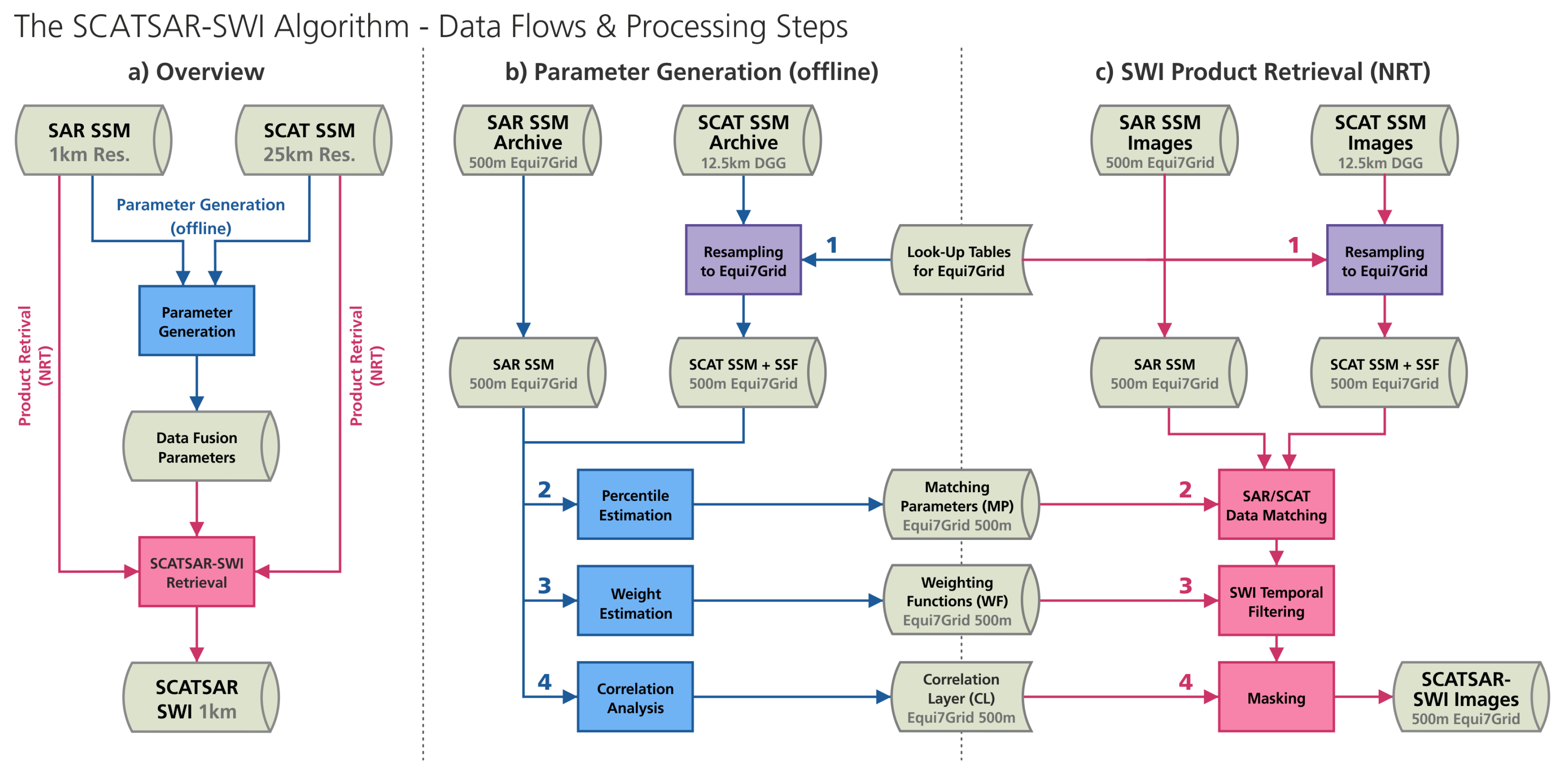
3. The SCATSAR-SWI Fusion Algorithm

The SCATSAR-SWI product is built on a fused data cube comprising SSM data from ASCAT and S-1. In general, the SCATSAR-SWI retrieval algorithm consists of two components: (1) an offline operated data fusion parameter generation, and (2) a NRT-capable SWI product retrieval, taking up the incoming SSM and the beforehand generated data fusion parameters. To give an overview, Figure 2 outlines the general structure of the algorithm.

3.1. SCATSAR Data Cube

Modern remote sensing places high demands on processing- and storage- facilities. It was found, for example, for S-1 that global-scale services in near-real-time (NRT) or reprocessing activities are only technically feasible when employed in High Performance Computing (HPC) environments due to the large daily data volume [60]. As a consequence, a modern remote sensing product retrieval algorithm is then required to support parallelised processing.

In recognition of these findings, the TU Wien GEO team developed an optimised data cube architecture for raster data from satellite sensors [61]. Its basic framework is the Equi7Grid [62], a spatial reference system designed to efficiently handle the archiving, processing, and displaying of high resolution raster data over land while preserving geometric accuracy. It is defined for the entire Earth and consists of seven planar subgrids for each continent, referenced to the ellipsoidal WGS84 datum. The coordinates are defined by individual realisations of the Equidistant Azimuthal projection, given as eastings and northings in metres. The Equi7Grid not only allows to conveniently handle large remote sensing spatio-temporal data, but also to relate and transform data of diverse spatial scales [63]. The Equi7Grid definitions and tools are available at [64].

Naturally, such a data cube approach is also well suited for the SCATSAR-SWI data fusion, since not only parallel image operations as well as time series analyses are facilitated, but also the combination of datasets from different scales is supported. Consequently, the spatial reference system for SCATSAR-SWI data cube is a Equi7Grid, realised with a sampling distance of 500 m (to allow a nominal spatial resolution of 1 km) and a regular square tiling with a 600 km extent. This choice was found to be optimal for the data handling in terms of file number and size, using LZW-compressed (Lempel–Ziv–Welch lossless data compression) geotiff-files organised per Equi7Grid-tile in image stacks.

The data fusion parameter generation requires a priori SSM datasets from SCAT and SAR, which together cover a multi-year period in order to allow robust estimates of the parameters. The SCATSAR-SWI data cube formed for this study (Section 5.1) holds SSM archives from ASCAT and S-1 for the period October 2014 to October 2017. For the same period, we generated the SWI product that is evaluated in Section 5.

SCAT Resampling

The S-1 SSM product is natively in 500 m-sampled Equi7Grid, hence this data can be directly ingested in the SCATSAR-SWI database, with no resampling action required. Contrary, the ASCAT SSM data is provided per satellite orbit segments as highly-compressed Eumetsat-BUFR files that are referenced to the WGS84 ellipsoid. Hence, a decoding and resampling of the ASCAT data is necessary. For the ingestion of ASCAT SSM data into the data cube, an oversampling of the 12.5 km-sampled data to the 500 m Equi7Grid-tiles is performed, employing the radial basis interpolation module of scipy using the “thin_plate”-function [65]. Despite the large oversampling factor of 25 (from 12.5 km to 500 m), the data volume is not inflated thanks to the efficient file compression. The mapping functions of ellipsoidal- to Equi7Grid- coordinates are constant and are read from precomputed Look-Up-Tables (LUTs) in order to speed up the ASCAT data resampling.

3.2. Data Fusion Parameter Generation

To ensure a valid fusion of the SCAT and SAR inputs, data fusion parameters are required to account for their different observation scale, accuracy, and local dynamics. We realise this with a set of static parameters retrieved from the S-1 and ASCAT archives covering 2014–2017, which are presented in the following subsections.

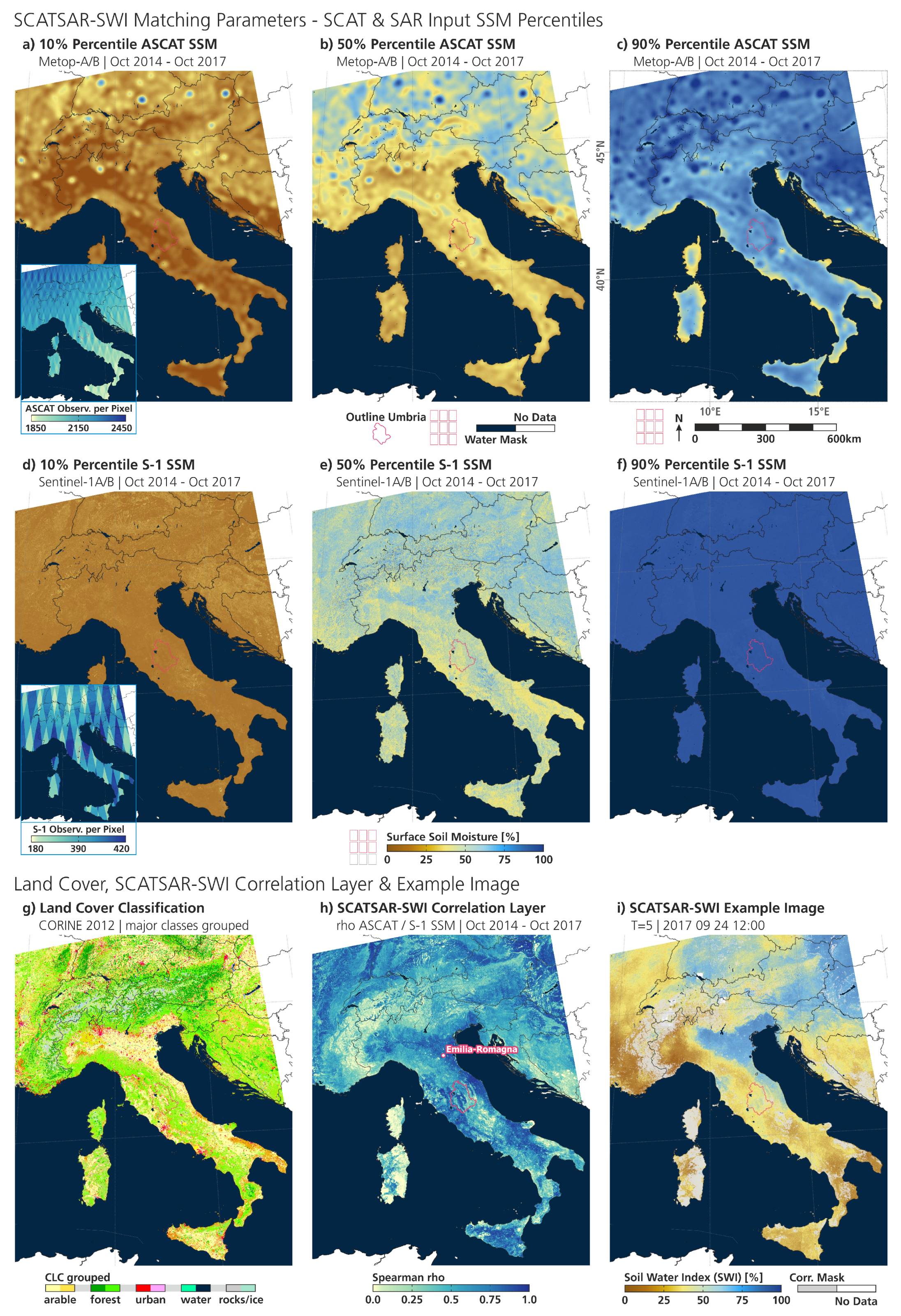
3.2.1. Matching Parameters

Both SSM products from SCAT and SAR are supposed to describe the same physical parameter, and they are retrieved from radar backscatter data that is recorded by comparable technologies. However, systematic biases are likely to occur due to sensor- and retrieval- specifics and the different complexity at the original scale, evoking land-cover-like patterns. The fusion of SCAT with SAR SSM should account for these systematic differences in order to obtain a consistent SM dataset.

Here, we use data matching per each grid point to obtain SSM signals with compatible levels and dynamics. Data matching techniques are methods to resolve signal biases and different signal variances in a dataset containing disparate sources [66] and thus meet our needs. There is a large set of data matching methods, among which the Cumulative Distribution Function (CDF) matching is widely used for soil moisture applications [43,67]. More specifically, CDF-matching can transform the mean, variance, skewness and kurtosis of a time series to approximately match the ones of the reference time series at relative low computational costs.

We realise the CDF-matching through a piecewise-linear matching of the SSM percentiles at each grid point. This requires a per-pixel signal analysis of the SAR and SCAT SSM archives, estimating the SSM percentiles in intervals of ten percent from 10% to 90%. These values form the Matching Parameters (MP) and are used then later during the SWI retrieval (Section 3.3.1).

3.2.2. Weighting Functions

The quality of input SSM data from SCAT and SAR is not necessarily equal and can vary over time. To regulate the impact of the input quality on the SCATSAR-SWI, we introduce weights for SCAT ($w_{SCAT}\left(t_p\right)$) and SAR ($w_{SAR}\left(t_p\right)$) that define the weight of the individual SSM values in the SSM history for the SWI estimation.

The quality can be characterised either by empirical estimates of the operator for the data quality, or by quantitative measures, e.g., through their signal error noise values $ϵ\left(t\right)$. The weights can be then realised through the inverse values of $ϵ\left(t\right)$, which form the Weighting Functions (WF) for SCAT and SAR SSM.

Alternatively, as a most simple implementation, only two static weights are defined for all SCAT and SAR values, respectively, identical for every grid point and for every point in time. In this study, we decided to use such static weights, owing to the large imbalance in temporal coverage between SCAT and SAR during the ramp-up-phase of S-1 in the years 2014 and 2015, giving much uncertainty to the error noise estimation. We set globally for all locations

$$\begin{array}{c}{w}_{\mathrm{SCAT}}\left(t\right)\to w_{\mathrm{SCAT}}{w}_{\mathrm{SAR}}\left(t\right)\to w_{\mathrm{SAR}},\end{array}$$

(3)

$$\begin{array}{c}{w}_{\mathrm{SCAT}}=w_{\mathrm{SAR}}=1,\end{array}$$

(4)

which virtually gives ASCAT much weight in the obtained SCATSAR-SWI product because ASCAT (A + B) has a 2–10 times higher revisit frequency than S-1 (A (+B)) over European locations and thus ASCAT SSM constitutes the majority of the SSM observations of the fused SSM data cube. With this setup, the SCATSAR-SWI processing takes in a simple way into account the higher average accuracy of the ASCAT SSM data, which is more mature [31].

3.2.3. Correlation Layer

The SCAT and SAR sensors observe in completely different spatial scales. Consequently, the observed radar signals are likely to describe different geophysical processes when spatial heterogeneity on the SAR-scale is given. Fragmented land cover may affect the finer SAR observations very differently than the coarse SCAT observations. However, if both input SSM signals therefrom feature similar temporal dynamics, it can be assumed that they describe the same SM process (invoking the temporal stability concept). To identify grid locations that fulfil this assumption, a Correlation Layer (CL) is built, holding for each grid point the correlation between the SCAT and the SAR SSM time series. The CL can then act as mask during the SWI production, flagging pixels where the correlation is low and thus not eligible for the SWI data fusion.

We calculate the Spearman Rank Correlation Coefficient $\rho$ at each grid point between the ASCAT and S-1 time series—after temporally matching them (yielding two samples of the same size). Additionally, the correlation significance is calculated to account for the sample size of the investigated time series. The CL holds for each grid point then two values, the $\rho$-value and the corresponding significance (p-) level.

3.3. SCATSAR-SWI Estimation

With a data fusion parameters ready, the SCATSAR-SWI can be calculated. In the following, we describe the methodology for an ongoing and near-real-time production of daily SWI images, which involves SCAT/SAR data matching, the SWI retrieval, and output masking.

3.3.1. SSM Distribution Matching

Following the argumentation discussed already in Section 3.2.1, prior to temporal filtering, the SSM data from SCAT and SAR should be matched. While the SCAT data is superior in capturing the temporal SM dynamics, the SAR product features much finer spatial dynamics, enabling the resolving of SM patterns on the kilometric scale.

Per 500 m Equi7Grid-grid-pixel, we match the previously oversampled ASCAT SSM (see Section 3.1.1) to the local S-1 SSM distribution. This is done through CDF-matching employed on the SSM percentiles generated as described in Section 3.2.1. At each grid point, the CDFs of ASCAT and S-1 SSM are approximated piece-wise through linearisation between the 10%-percentiles. Each ASCAT SSM value is then mapped from the local ASCAT CDF to corresponding S-1 CDF segment, resulting in an ASCAT SSM image settled on the spatial definition of the SAR record. In this way, we disaggregate the coarse-scaled SM observation and adapt it to the fine-scaled SM patterns.

3.3.2. Recursive Weighted Temporal Filtering

The calculation of the SWI values using the approach introduced in [40] requires the availability of historic SSM time series data (Equation (2)). A computational adaption of the algorithm towards ongoing, day-to-day SWI production has been proposed already in [68]. They found a recursive reformulation of the SWI calculation that is mathematically equivalent to Equation (2). Using their formulation, recasting the terms and shifting the time indexing by 1, we found an alternative expression of their recursive calculation. The SWI for a given characteristic time length T can then be derived using the formula:

$${\mathrm{SWI}}_T\left(t_{i+1}\right)={\mathrm{SWI}}_T\left(t_i\right)+\frac{\mathrm{SSM}\left(t_{i+1}\right)-{\mathrm{SWI}}_T\left(t_i\right)}{de{n}_T\left(t_{i+1}\right)},$$

(5)

where $t_i$ refers to the time of the previous, and $t_{i+1}$ of the current SSM measurement, so that ${\mathrm{SWI}}_T\left(t_i\right)$ is the SWI at the time of the previous SSM measurement and $\mathrm{SSM}\left(t_{i+1}\right)$ is the new SSM measurement. The so-called denominator factor $de{n}_T\left(t_{i+1}\right)$ expresses the time-dependent filtering and is calculated from the previous denominator factor as

$$de{n}_T\left(t_{i+1}\right)=1+e^{-\frac{t_{i+1}-t_i}{T}}de{n}_T\left(t_i\right).$$

(6)

Hence, the difference of the current SSM to the previous SWI (the nominator in Equation (5)) and the filtered time delta (the denominator in Equation (5)) determine the next SWI value.

Evidently, for the recursive calculation, the last SWI value and the last denominator factor need to be stored. Then, the calculation can be continued at any time, practically when new input SSM data are available from SCAT or SAR, or as we implement it, everyday at 12:00 UTC. In our case, all SSM values from the past 24 h are consecutively converted to SWI values with Equation (5), whereas the last SWI value of the 24 h is stored in the output SWI image of that day. The calculation of SWI is initiated at time $t=0$ with the following values:

$$t_i=t_{i+1}=0,{\mathrm{SWI}}_T\left(0\right)=\mathrm{SSM}\left(0\right),de{n}_T\left(0\right)=1.$$

(7)

Our alternative recursive SWI calculation introduced in Equation (5) is convenient when it comes to (quality-) weighted SSM values, which we implement for the SCATSAR-SWI to weight individually the SCAT SSM and SAR SSM input values. To begin with, we add $w\left(t_i\right)$ as weight for $\mathrm{SSM}\left(t_i\right)$ and n for the cumulative total number observations, and expand the Equation (2) to the Weighted SWI formulation:

$${\mathrm{SWI}}_T^w\left(t_n\right)=\frac{n{{\displaystyle \sum }}_{i=1}^{n}w\left(t_i\right)\mathrm{SSM}\left(t_i\right)e^{-\frac{t_n-t_i}{T}}}{{{\displaystyle \sum }}_{i=1}^{n}w\left(t_i\right){{\displaystyle \sum }}_{i=1}^n{e}^{-\frac{t_n-t_i}{T}}}\mathrm{for}{t}_i\le t_n.$$

(8)

The above equation uses the complete SSM history. For SWI retrieval in ongoing, day-to-day processing, we need, however, the recursive calculation of the Weighted SWI. The ${\mathrm{SWI}}_T^w$ can be recursively calculated as:

$${\mathrm{SWI}}_T^w\left(t_{i+1}\right)=\frac{{\mathrm{SWI}}_T^w\left(t_i\right)\frac{n+1}{n}{\displaystyle \sum }{w}_i(de{n}_T\left(t_{i+1}\right)-1)+\mathrm{SSM}\left(t_{i+1}\right)(n+1)w\left(t_{i+1}\right)}{{\displaystyle \sum }{w}_{i+1}de{n}_T\left(t_{i+1}\right)},$$

(9)

where ${\displaystyle \sum }{w}_i$ and ${\displaystyle \sum }{w}_{i+1}$ represent the previous and current cumulative sum of weights, respectively (with ${\displaystyle \sum }{w}_{i+1}={\displaystyle \sum }{w}_i+w\left(t_{i+1}\right)$). Consequently, ${\displaystyle \sum }{w}_{i+1}$ needs to be stored together with the denominator factor $de{n}_T\left(t_{n+1}\right)$ and the number of total observations ($n+1$) for the next calculation at time $t_{i+2}$. It is worth noting that the weights are not required to be normalised.

3.4. Output Masking

There are two maskings in the SCATSAR-SWI. First, the surface state flag, coming from the ASCAT SSM product (SSF, [55]), identifies frozen conditions. The SCATSAR-SWI algorithm discards SSM estimates when the SSF is not “unfrozen” and reduces an internal, T-value-dependent quality flag. An ongoing period of no valid SSM values leads to gaps in the dataset also after frozen conditions, as the quality flag needs to recover, assuring that no values measured under frozen conditions are part of the used SSM history $W_{SL}\left(\tau \right)$. All this is done on the ASCAT grid, hence the data gaps are block-shaped and ca. 12.5 km large. SSF-masked gaps mostly occur in alpine or cold climates during the cold season.

Second, we apply the Correlation Mask (CM) that is retrieved from the Correlation Layer (CL), as the SCATSAR-SWI should only be used where the SCAT and SAR reasonably agree. Following Section 3.2.3, the CM is defined through a threshold of minimum correlation and significance, yielding a logical mask on the 500 m-pixel-grid.

4. Evaluation Datasets and Methods

4.1. SCATSAR-SWI Production

For evaluating the SCATSAR-SWI retrieval method, we generated a 3-year dataset over Italy, using all available Metop-A/B-ASCAT and S-1A/B observations from October 2014 to October 2017. From the fused SSM data cube, we generated the parameters as described in Section 3.2, yielding a set of matching parameters, correlation- layer, and -mask per Equi7Grid-tile. With that, we retrieved the SCATSAR-SWI images for each day in the period October 2014–October 2017. We masked the output data for water bodies using the mask included in the S-1 SSM product, and for low SCAT-SAR correlation using the Correlation Layer with $\rho =0.3$ as lower limit.

4.2. Layout of Experiments

A comprehensive evaluation of remotely sensed SM data requires reference datasets of comparable spatio-temporally density and coverage [50,69]. Having said this, comparisons of remotely sensed observations with in situ data is often troubled by dataset inconsistencies and a scale-mismatch [70]. In order to complement the evaluation against in situ data, we used in this study the Soil Water Balance Model (SWBM, [71]) and carried out an in-depth analysis of the signal quality over the Umbria region in central Italy, validating the SCATSAR-SWI data against the model data, as well as against reference from ASCAT and available in situ observations. Furthermore, we used the SM2RAIN approach [8] to evaluate the skill of the SCATSAR-SWI to record the impact of rainfall on SM. For this, we compared daily mean rainfall observations over Italy, and in detail over Umbria, against estimates from the SM2RAIN algorithm ingesting our SCATSAR-SWI data.

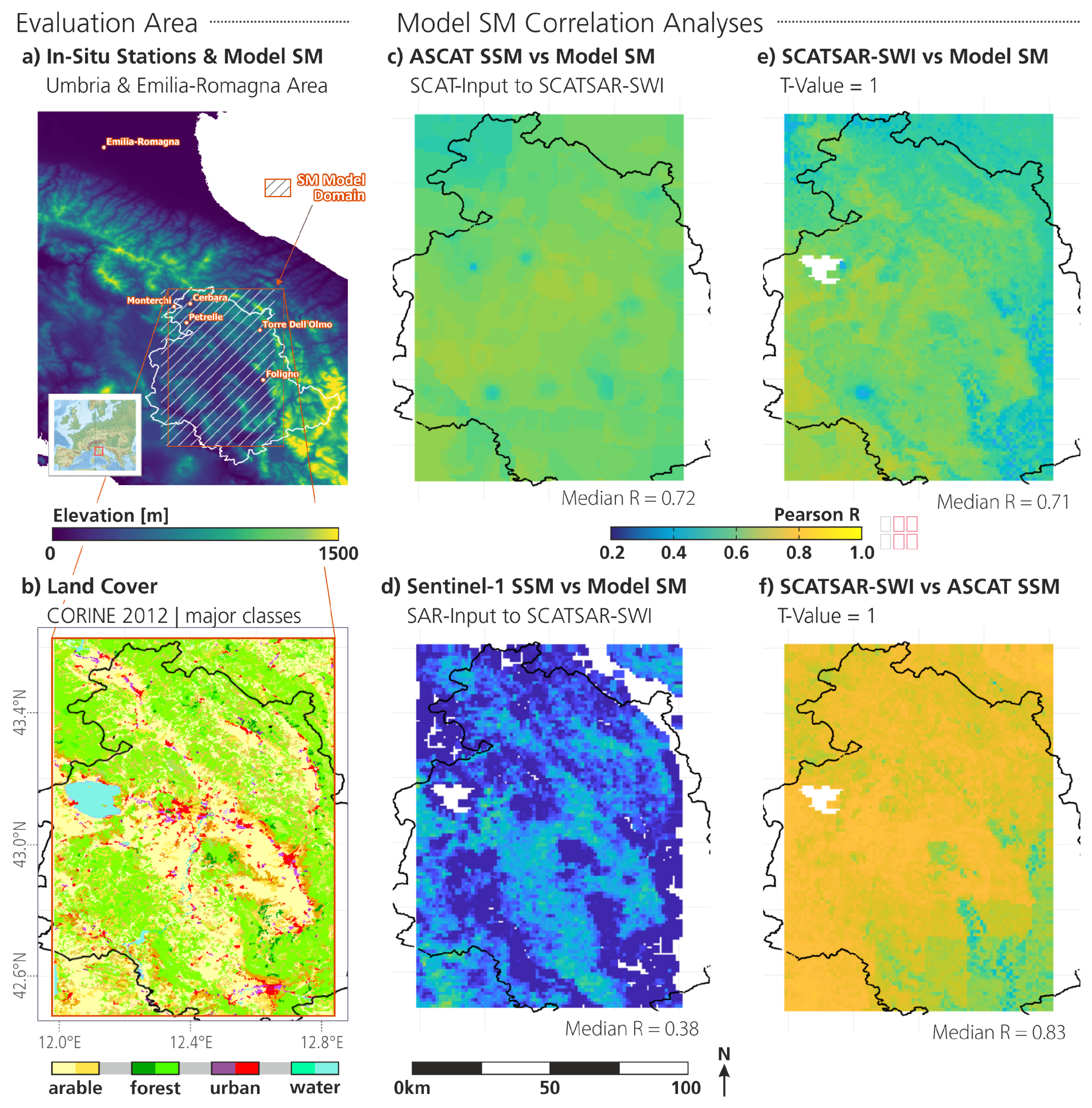
4.3. Study Area: Umbria Region

The Umbria region is located in central Italy and it is characterised by a complex landscape topography. Land uses are mainly forests (42.6%), and crops (49.2%), with urban areas covering only 3.5% of the territory. See in Figure 3a the region’s topography, and in Figure 3b its land cover as from CORINE 2012 [72]. The climate is Mediterranean, with mean annual rainfall of 950 mm and mean annual air temperature ranging between 3.5 ${}^{\circ }$C and 14.0 ${}^{\circ }$C.

A dense real-time hydro-meteorological network (90 rain gauges, 77 thermometers, one station every 150 km${}^2$) has been operating for more than 20 years and 12 soil moisture stations distributed throughout the territory [73]. The monitoring network provides semi-hourly data for which a quality-check step is performed in order to remove anomalous values and to fill any temporal gaps.

4.4. Model SM Data: SWBM-SA Umbria

We used modelled 1 km soil moisture (Model SM) estimated with semi-analytical SWBM (SWBM-SA [74]) to test the ability of the SCATSAR-SWI data to reproduce the temporal and the spatial variation of SM at the 1 km-scale. The SWBM was specifically developed to reproduce in situ SM observations in the Umbria region [71], and has been successively applied also in different test-sites across Europe yielding satisfactory results, with correlations higher than 0.8–0.9 and Root Mean Square Differences (RMSDs) lower than 0.025 m${}^3/$m${}^3$ [45,74,75,76].

For this study, interpolated 1 km rainfall and temperature data drove the SWBM-SA model, yielding hourly-based SM estimates on a 1 km-based regular grid for an area of 8991 km${}^2$ (Figure 3a). The mountainous eastern part of the region was intentionally excluded as the density of rain gauges here is much lower and the satellite observations are expected to be largely impacted by the topography. Input precipitation and temperature data cover the period 2014–2017. Model parameters are obtained from soil texture information available over the study region (outlined in [73]). SM estimates were modelled for the topmost 10 cm of the soil to match the depth of the SCATSAR-SWI at T-value of 1 and 5, following the study of [41].

4.5. In Situ SM Data: ISMN

In situ data from the International Soil Moisture Network (ISMN, [77]) were used for evaluation (In Situ SM). The ISMN provides a harmonised repository of in situ SM observations all over the world and is well-evaluated and established in the community [41,78,79]. Here, we use five UMBRIA-stations from the Umbria region and one COSMIC-station, close-by in the Emilia-Romagna region (see Figure 3a).

During the analysis period, only five out of twelve UMBRIA-stations measured soil moisture, some of them discontinuously, or not during the full period. The five instruments consist of four Frequency Domain Reflectometry (FDR) stations and one Time Domain Reflectometry (TDR) station with sensors located at different depths (5–40 cm). Three stations (Cerbara and Torre dell’Olmo and Petrelle) are operating in real-time and provide measurements every 30 min. For the validation of SCATSAR-SWI data, we used only the at all stations available topmost measurements at a depth of 10 cm. The two stations in the east of Umbria are located in a section of good coverage by S-1 (Foligno, Torre Dell’Olmo with 401 measurements), the other three in the northwest were measured only half as often (Cerbara, Monterchi, Petrelle with 198 measurements).

The COsmic-ray Soil Moisture Observing System (COSMOS) is a network of stations that measure soil moisture through a newly-developed cosmic-ray method [80]. The stationary cosmic-ray soil moisture probe measures the neutrons that are generated by cosmic rays within air and soil and other materials, moderated by mainly hydrogen atoms located primarily in soil water, and emitted to the atmosphere where they mix instantaneously at a scale of hundreds of metres and whose density is inversely correlated with soil moisture. This measurement scale makes it a valuable reference for the remotely sensed and 500 m-sampled SCATSAR-SWI.

We used the station Water4Crops Budrio IT (098), located in Emilia-Romagna in the Po Valley in an extremely flat area with intensive, irrigated agriculture. It is a test site for different irrigation techniques and different water sources (reuse of treated wastewater) and has a mean annual precipitation of about 750 mm with a mean annual temperature of 16.0 ${}^{\circ }$C. The station provides measurements of soil moisture in the range of 0–21 cm and data are available from about 2014 to 2016. This station is located in section of medium S-1 coverage (286 measurements).

4.6. Rainfall Observations

The assessment of the SCATSAR-SWI through SM2RAIN has been carried out at national scale (Italian territory) and local scale (Umbria region). The observational rainfall dataset for the Umbria region is already described in Section 4.3 and Section 4.4, and the Italy-dataset is obtained from an interpolation of 3000 rain gauges provided by the monitoring network of the National Civil Protection Department [81]. The hourly observations are spatially interpolated over the analysis grid at 3 km resolution by using the Random Generator of Space Interpolations from Uncertain Observations algorithm [82] and aggregated at a daily time step. The dataset is available from April 2015 to April 2016.

4.7. SM2RAIN from SCATSAR-SWI

The SM2RAIN algorithm was developed in [8] to obtain rainfall estimates from in situ and satellite SM observations. The algorithm has been applied extensively to several satellite SM products obtaining good performance in the reproduction of ground-based rainfall observations (see for most recent applications [83,84]). In this study, we applied SM2RAIN to SCATSAR-SWI with T-value = 1 by following the same approach as in [84] (the reader is referred to this paper for details). The SM2RAIN parameter values are calibrated against rain gauge observations described in Section 4.6 to obtain two rainfall products at daily time scale: (1) Italian scale product at 3 km spatial resolution for the period from April 2015 to April 2016, and (2) Umbria scale product at 1 km spatial resolution for the period from October 2015 to September 2016. For comparisons, a second SM2RAIN dataset was created with ASCAT SSM as input, using the same methods but a rainfall product calibrated at 10 km spatial resolution.

4.8. Data Preparations for Evaluation

The different SM products that are examined in the evaluation experiments are characterised by different measurement units and have different grids. Thus, we reprocessed them for a meaningful comparison. More specifically, the comparisons of SCATSAR-SWI and ASCAT SSM data with the reference data (in situ and model) required the following steps: (1) Spatial matching: The grid pixel of the SCATSAR-SWI and ASCAT SSM whose centroid is nearest to the reference location has been selected, and the corresponding relative SM time series has been extracted; (2) Temporal matching: The site-specific soil moisture data closest to the corresponding acquisition time of SCATSAR-SWI and ASCAT SSM were extracted from their time series. Flagged data due to water, frozen conditions (through ASCAT’s SSF), or out-of-bound values were masked out; (3) For the ISMN-comparison, a conversion to volumetric SM units is necessary: per pixel, the mean and the variance of SCATSAR-SWI and ASCAT SSM (both in relative units) were matched with those of co-locating reference data to obtain absolute values in m${}^3$ m${}^{-3}$, following [85].

Accounting for the temporal frequency of S-1 observations of 1.5 to 4 days over the study area, the correlation analysis of the SM2RAIN-derived rainfall products is carried out for five-day accumulated rainfall.

5. Evaluation Results and Discussion

We evaluated SCATSAR-SWI data over Italy against reference soil moisture data from the model-, satellite-, and in situ-datasets, as well as rainfall data, following Section 4.2.

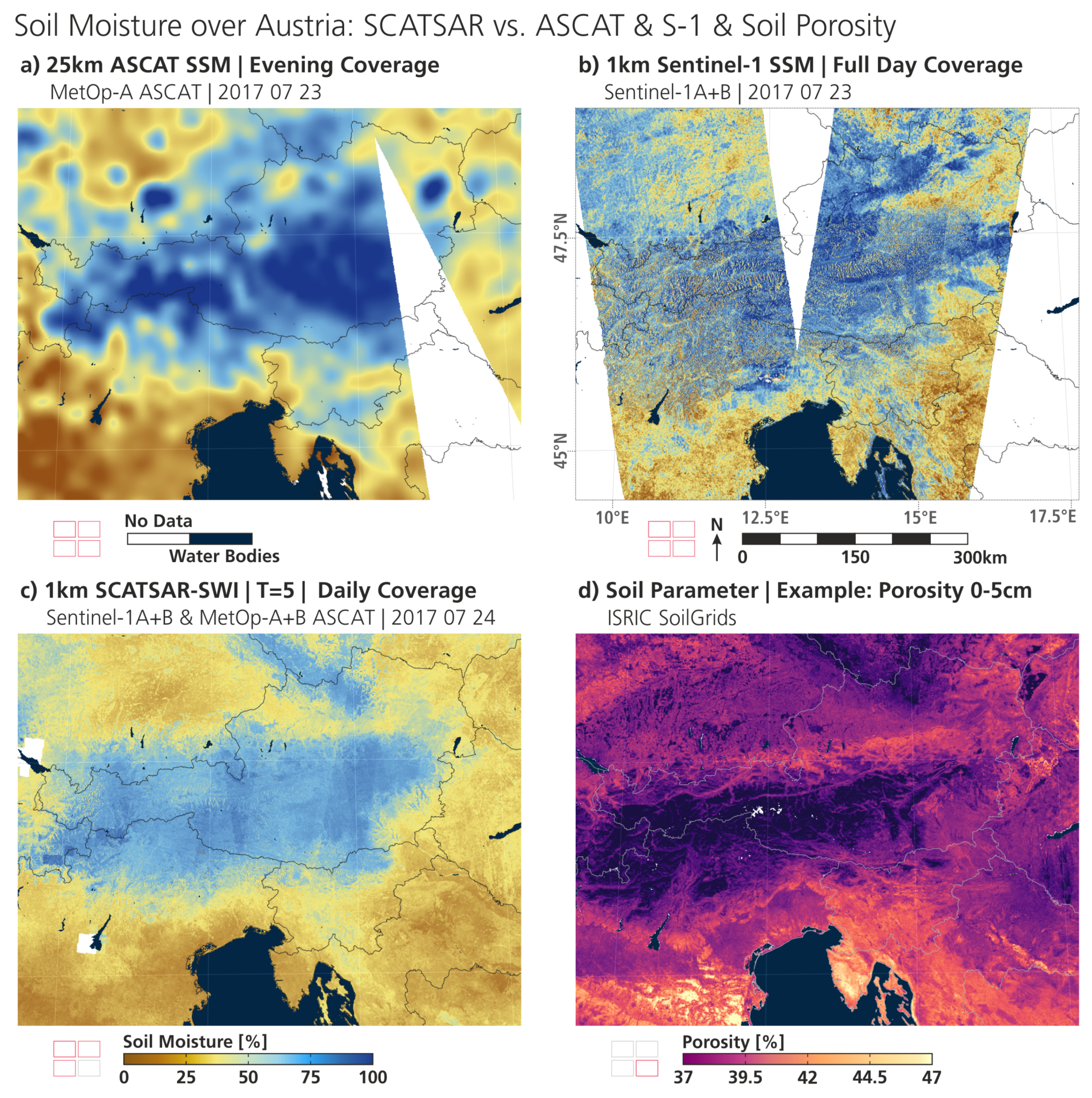
5.1. The SCATSAR-SWI Dataset

For the evaluation presented here, all available ASCAT and S-1 SSM observations over Italy and its neighbours were processed with the algorithm in Section 3 and the setup outlined in Section 4.1. The obtained data cube consists of SWI daily imagery over five Equi7Grid-tiles (each 600 km wide). The SCATSAR-SWI data is built up of 180 to 420 single observations per 500 m pixel from S-1 SSM (average 292), and of 1850 to 2450 from ASCAT SSM (average 2060), depending on the S-1 and ASCAT orbit coverages (see minimaps in Figure 4a/d). As one can see, the S-1 coverage is very inhomogeneous, which is directly resulting from the Sentinel observation scenario [31]. For the first two years during the period (October 2014 to October 2016), ASCAT features, on average, a seven times higher frequency than S-1, as the ASCAT satellites overpassed an average location 2.2 times a day and S-1 only 0.3 times a day. From October 2016 onwards, the S-1 mission is in full deployment using two satellites. With the inclusion of S-1B, twice as much S-1 SSM measurements are available over Europe, with ASCAT featuring then a 3.5 times higher frequency than S-1. Overall, the fused SSM dataset consist of ca. 80% ASCAT observations.

To give a first impression of the data, Figure 5 compares the SM patterns of the input SSM from ASCAT and S-1, and the SCATSAR-SWI with T-value = 5 for 23 July 2017. Figure 5d adds the porosity of the soil layer at 0–5 cm depth from ISRIC SoilGrids [63] to the comparison. On that day, ASCAT achieves almost full coverage over the area with evening overpasses alone, while S-1 morning and evening overpasses cover less area (and has no coverage on the next day (not shown)).

As obvious from Figure 5, the S-1 SSM and SCATSAR-SWI feature a much higher degree of spatial detail than the ASCAT SSM. Accordingly, the comparison with ISRIC data illustrates that the two kilometric products are much closer to the scale of soil characteristics. However, both SSM signals seem to be contained in the SWI, as the smooth patterns from ASCAT and also the detailed patterns from S-1 are reflected in the SWI (e.g., in southeastern Austria or in the border area of Slovenia and Croatia). Ideally, the SCATSAR-SWI provides a resolution of 1 km as a result from the SCAT data matching and the SAR signal contribution. However, the actual resolution of the present SCATSAR-SWI appears to be lying between the resolution of S-1 and the ASCAT input, owing also to the large share of ASCAT observations in the fused data cube.

Interestingly, typical wet biases over large cities are apparent as blue spots in the ASCAT data, e.g., over Vienna (northeast in Figure 5a) or Munich (northwest), which are completely rectified in the SCATSAR-SWI. It is also noticeable that the SCATSAR-SWI contains linear artefacts following the edges of ASCAT and S-1 orbit footprints. These artefacts are due to different timings of the inherent SSM observations in adjacent image sections. Such linear artefacts are already known from the 12.5 km ASCAT SWI (not shown, e.g., as available from Copernicus Global Land Service (CGLS) [86]) at lower T-values, but appear to be more pronounced in the SCATSAR-SWI. In a sense, their perceptibility result from migrating the SWI method from the coarse scale, which is usually displayed in a time-series domain, to a finer scale, which is usually displayed in the image domain.

The data fusion parameters are an important part of the SCATSAR-SWI retrieval. Figure 4 displays the SCATSAR-SWI Matching Parameters and the Correlation Layer, together with CORINE Land Cover and an example SCATSAR-SWI image over Italy and its neighbours, with the Umbria region in central Italy marked out. In addition, the ASCAT and S-1 satellite coverages are plotted as mini-maps that show total SSM observations during the evaluation period.

Figure 4a–c show the 10%-, 50%-, and 90%-percentiles of the ASCAT SSM input dataset, representing statistically low, average and high SSM during the period October 2014 to October 2017. The coarse resolution of this product is eminent, as no detailed features, e.g., in the scale of the land cover in Figure 4g, can be resolved with the ASCAT data. Moreover, along the coasts, drier SSM values occur that are potentially wrong, commonly owed to mixed sea/land backscattering effects in the large ASCAT footprints (exceedingly over Sardinia and Corsica). In addition, the wet biases over cities are obvious in all ASCAT SSM percentiles, especially in the northern section of the maps. One explanation for this could be the growth of urban areas during the ASCAT period from 2007 onwards, troubling the parametrisation of the ASCAT model in areas with soil turning into artificial surfaces, or with increasing built-up density. The 50%-percentile (median) map indicates that the period 2014–2017 was drier than normal in Italy, southern France and the Adria region as here the median SSM is largely around 30–40%. With the years 2014–2017 being reported drier than the previous years, this deviation from 50% SSM stems from the different observation periods and resulting parametrisation baselines of ASCAT (2007–2017) and SCATSAR (2014–2017). As the latter is identical with the S-1 observation period, S-1 features largely uniform SSM values in the 10%-, 50%-, and 90%-percentile maps in Figure 4d–f.

The Correlation Layer (CL) in Figure 4h holds the Spearman correlation coefficients between input SSM from ASCAT and S-1 for each pixel. The parameter is essential to the SCATSAR-SWI, as the SWI should be used only at locations with a reasonable good agreement between SCAT and SAR. The CL acts as a descriptor of how well the unlike-scaled signals of ASCAT and S-1 data match and thus indicates where the temporal stability concept for soil moisture is applicable. Indeed, the spatial patterns of the CL reflect many features in the CORINE land cover (as in Figure 4g), featuring, for example, rivers and cities. The CL shows generally high values over arable land, where large forests are absent, e.g., in the Po Valley in central-northern Italy, most of Sicily, the Rhine Valley at the French-German border area, or north and east of Vienna. Contrary, areas with a rough topography (e.g., the western Alps, the Apennines in central Italy, or Corsica and Sardinia) show very low values, due to a generally large geographical heterogeneity there. Similarly, areas with diverse land cover, with forests and agriculture mixed at the kilometre scale as, for example, Calabria in southern Italy, Tuscany west of Umbria, or southern Croatia and Bosnia show low values too. Large contiguous forests, however, like over the Apennines in northern Italy or over the eastern Alps in southern Austria, show medium correlation, further suggesting that spatial complexity governs the temporal stability.

Finally, Figure 4i shows an example SCATSAR-SWI image for 24 September 2017 at 12 h, with the Correlation Mask (CM) applied. The SWI (at T-value = 5) shows wet top soil layer conditions in the Po Valley and Venetia, over eastern Austria, western Hungary and Slovakia, and dry conditions over southeastern France, Piedmont, and southern Italy. Neither dry biases along the coasts nor wet biases around cities seem to be present, suggesting a successful data matching of the ASCAT signal. In addition, the spatial detail of the SAR input is preserved to some extent, while its noise is largely removed. The SWI images features well-defined SM gradients, for instance at the southern fringe of the Alps in north-eastern Italy. The CM (with $\rho =0.3$ set as threshold) takes out pixels over the western and central Alps, large sections in Sardinia and Corsica, and more scattered, over central and southern Italy, and southern Croatia and Bosnia. Two square-like gaps in the Alps result from the ASCAT’s SSF-flagging (done at the 12.5 km grid) that masks these locations (which in this case have a large share in water-bodies and rocks) as not enough valid input SSM data were available.

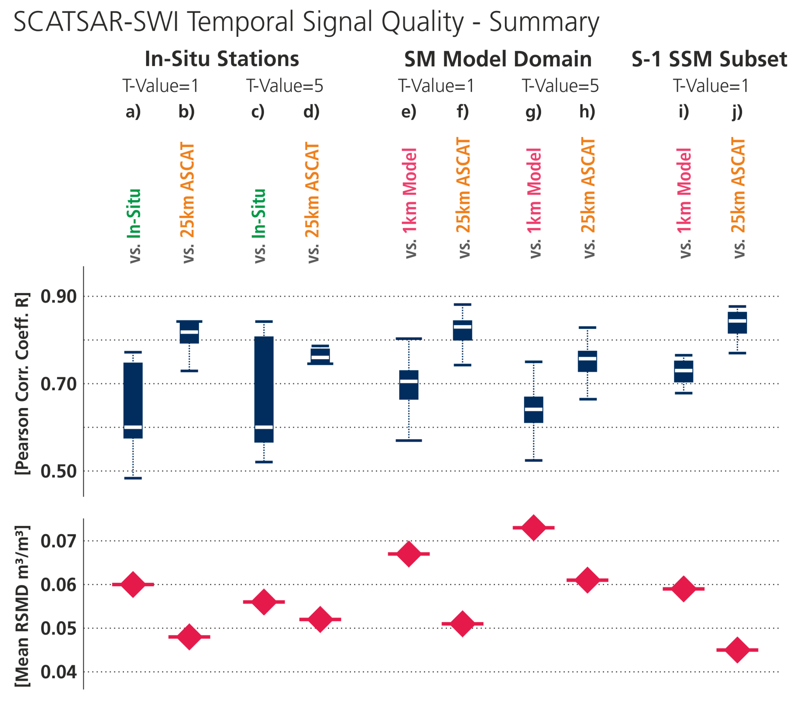
5.2. SCATSAR-SWI Signal Quality: Umbria Model Domain

Main results from the evaluation of the SCATSAR-SWI and its inputs against the Umbria model SM are displayed in Figure 3: Figure 3c is a map of the Pearson correlation coefficients (R) between the input ASCAT SSM and the model data, plotting 8991 1 km grid pixels. Obviously, ASCAT is uniformly agreeing well with the model, with a median R = 0.72. In contrast, the S-1 SSM input has a much lower average agreement with the model (Figure 3d, median R = 0.38) and shows a much more differentiated result, with low values over forests and high values over arable land as a comparison with the land cover in Figure 3b suggests. This behaviours of the S-1 SSM was already found in the recent study [31] and was related to the insufficient modelling of seasonal dynamics in vegetation density and its water content. However, the SCATSAR-SWI appears to be not much affected by this deficit of the SAR data, since it shows similar performance (Figure 3e, median R = 0.71) to the ASCAT product. The SCATSAR-SWI shows a less uniform pattern, with improved values over arable land (especially in the southwest) and decreased values over mountainous, forested areas in the southeast of Umbria. Not surprisingly, the correlation with the ASCAT SSM is (except for the mountainous southeastern area) very high and spatially consistent (Figure 3f, median R = 0.83), confirming that the ASCAT signal is successfully downscaled to the SCATSAR-SWI, devoid of quality degradation through, for instance, the data matching.

The results in Figure 3 discuss the SWI with T-value = 1, which is closest to the soil surface. The same analysis was done for T-value = 5, which represents SM just below the surface. Those results show as expected the same patterns (not shown) but slightly lower R-values (vs. model: median R = 0.64; vs. ASCAT: median R = 0.76) with the surface model data.

A separate statistical assessment was done for the area subset where the S-1 SSM input has a correlation higher than 0.5, mostly coinciding with zones in Umbria classified as arable (comparing Figure 3b,d). For this subset, the correlation is marginally better (vs. model: median R = 0.73; vs. ASCAT: median R = 0.84). ASCAT SSM shows a marginally lower agreement with the model over this subset (not shown, median R = 0.72), suggesting that the SAR component may not only add spatial detail but may also improve the temporal signal the SCATSAR-SWI over arable and flat areas.

The evaluation summary in Figure 6 plots the distributions of Pearson R and average root mean square difference (RMSD) for comparisons with in situ SM, ASCAT SSM, and model SM for both levels, at T-value = 1 and T-value = 5.

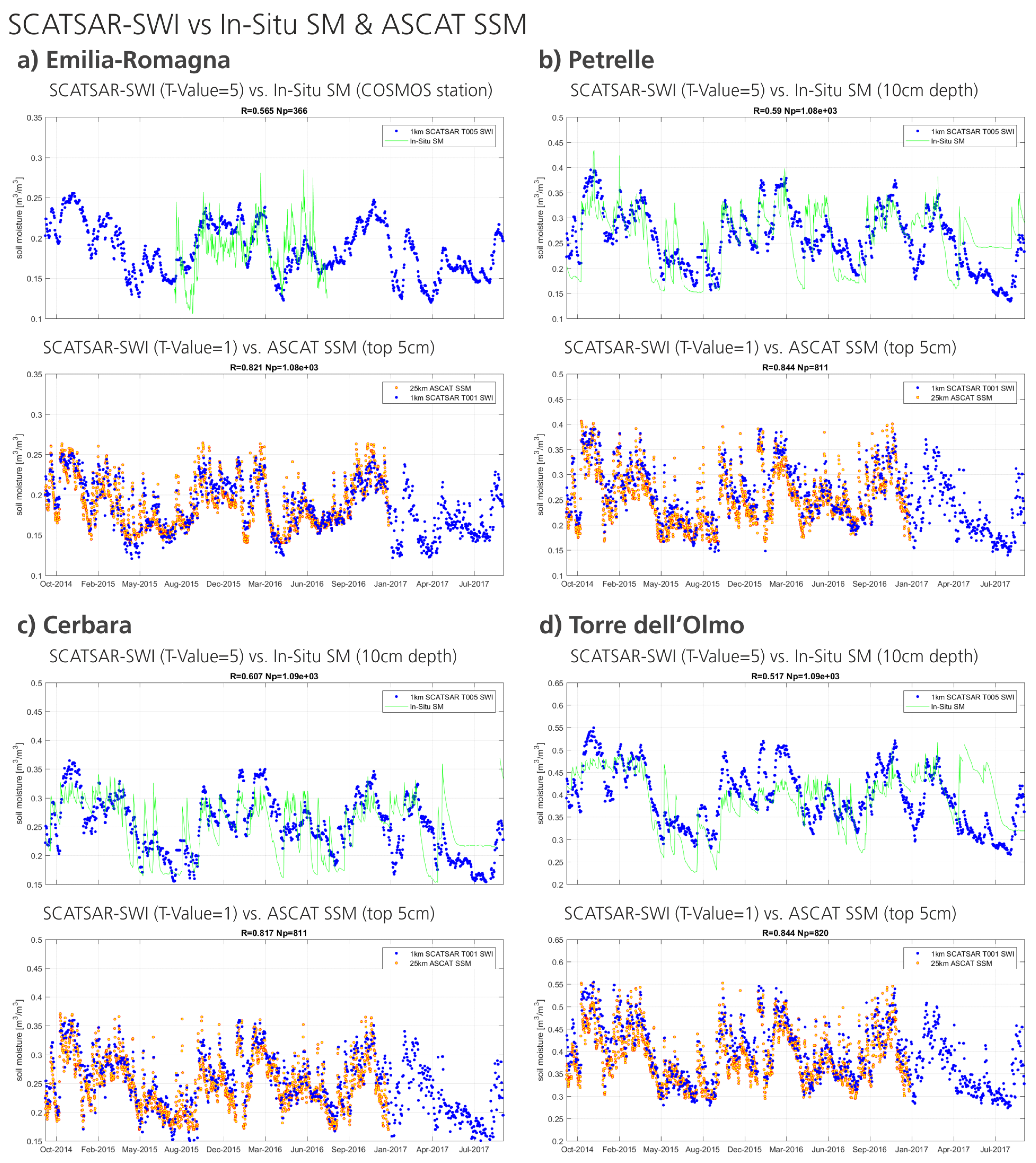
5.3. SCATSAR-SWI Signal Quality: In Situ Stations

Figure 6a–d collects results from the evaluation of the SCATSAR-SWI against the reference data at the in situ stations. Overall, the agreement in SM dynamics is good (T-value = 1: median R = 0.60; T-value = 5: median R = 0.61), and has an acceptable average accuracy (T-value = 1: mean RMSD = 0.060 m${}^3/$m${}^3$; T-value = 5: mean RMSD = 0.056 m${}^3/$m${}^3$). Comparisons against ASCAT SSM at the in situ locations show very high correlations (T-value = 1: median R = 0.82; T-value = 5: median R = 0.77) as expected, verifying the measured performance over the Umbria model domain. ASCAT SSM itself shows comparable, slightly better agreement with in situ observations and identical average accuracy (not displayed, median R = 0.63, mean RMSD = 0.056 m${}^3/$m${}^3$), indicating that the temporal dynamics of the ASCAT signal is forwarded intact to the SCATSAR-SWI data.

The SCATSAR-SWI time series at the locations of the ground stations are plotted in Figure 7 against in situ and ASCAT reference, illustrating the high agreement of the data. We chose SWI at T-value = 5 for the comparison with the in situ measurements, which represent subsurface SM, and SWI at T-value = 1 for the reference from ASCAT (Surface SM).

The signal from the COSMOS-station in Emilia-Romagna from July 2015–August 2016 is well reproduced by the SCATSAR-SWI (Figure 7a). The COSMOS data is not a point measurement but represents an area of some hundreds of metres radius and is hence of particular interest. While the SCATSAR-SWI shows some wet bias during December 2015, and a dry bias during the subsequent spring, which both may be the consequence from an uncertain conversion to absolute SM due to the short temporal intersect of the two datasets, it accurately reproduces the timing of rises and drops in SM. The amplitude of the SM signal is much larger in the COSMOS data, underlining that the satellite product is not capable of fully capturing SM dynamics at the sub-kilometre scale. However, the SM signal of the ASCAT SSM (Figure 7a bottom), which describes the much larger 25 km SM signal, is well reflected in the SCATSAR-SWI.

Similar observations can be made from the time series plots at the other in situ stations (Figure 7b–d). The amplitudes of the Petrelle and Cerbara ground data show a good match with the SCATSAR-SWI, while some peaks are less pronounced, and many drops are much sharper in the in situ time series. Here the questions remains to what extent this is due to insufficient modelling of the satellite data or because of the scale mismatch between pointwise in situ and extensive remote sensing data.

Interestingly, at Petrelle, Cerbara, and most pronounced at Torre dell’Olmo, the SCATSAR-SWI contradicts the ground measurements when indicating very dry conditions during summer 2017, which was reported to be a very hot and dry season in Italy. The constant values at Petrelle and Cerbara from May to August 2017, clearly above the dry level, are peculiar and leaving doubt if irrigation measures or sensor issues may play a role here.

The above findings are widely supported by the time series analyses at the remaining two stations, which are included in the statistics in Figure 6 but not shown in the time series plots in Figure 7.

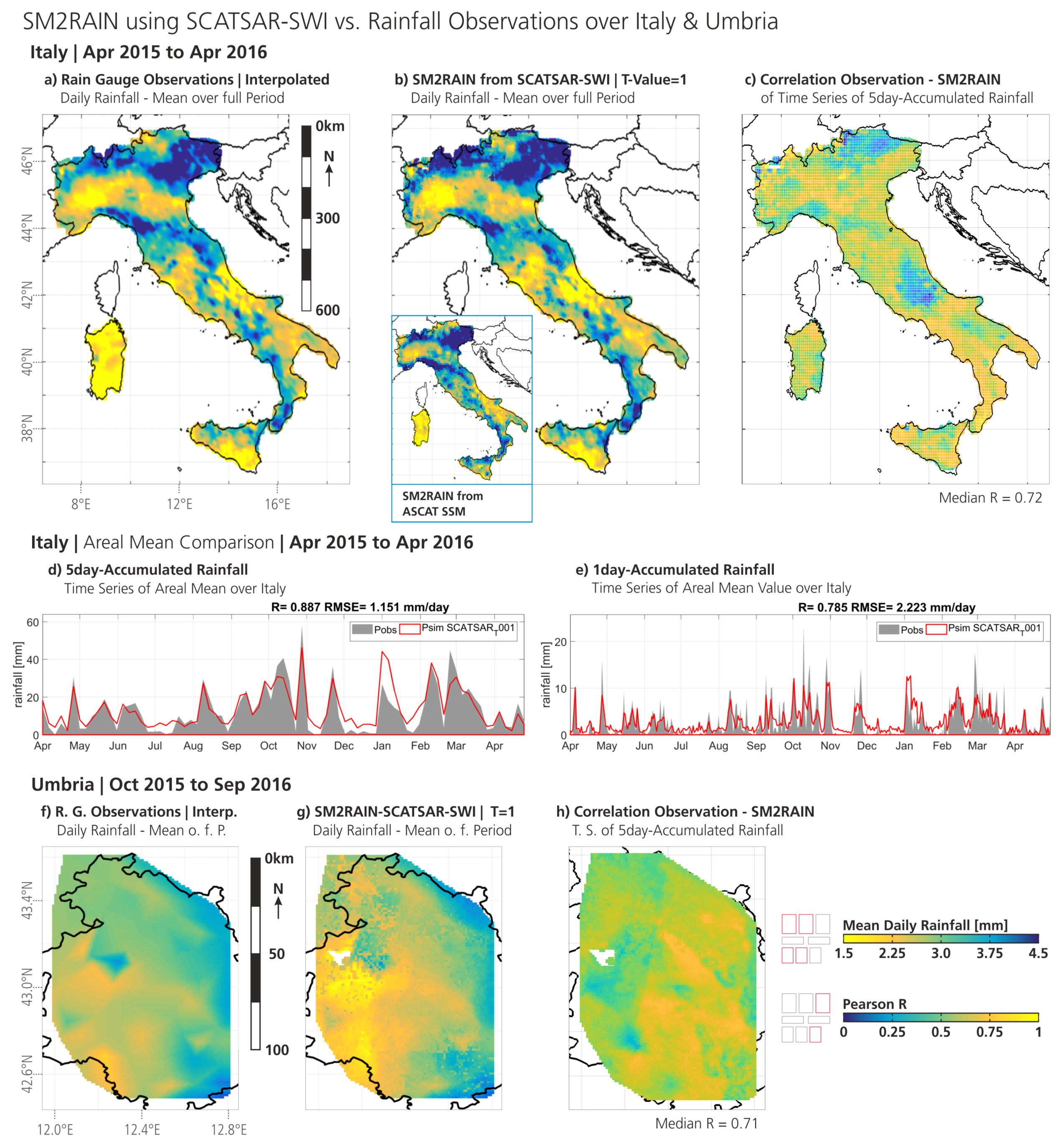
5.4. SCATSAR-SWI Rainfall Estimates over Italy

The experiments where we used the SCATSAR-SWI as input for the rainfall retrieval using the SM2RAIN method yielded very promising results (Figure 8). The first experiment, generating daily rainfall estimates at a 3 km sampling over entire Italy during the period April 2015–April 2016, reproduced the rainfall observations very well, as the average maps for this period almost coincide (Figure 8a,b). The correlation map between the five-day-accumulated rainfall from observations and SM2RAIN report values higher than 0.75 for a large part of Italy (median R = 0.72). Most notable regions with lower agreement are Alto Adige in the north and the Abruzzi in the centre, which are both of mountainous character.

The temporal evolution of the 5 day-accumulated areal mean for Italy (Figure 8d) also shows a very high agreement between observations and SM2RAIN estimates (R = 0.89, RMSE = 1.15 mm/day). Only during the winter period in December 2015 and January 2016, and to a lower degree during July 2015, one can see the five-day rainfall sums differ. The deviations during the cold period may result from incorrect detection of frozen/snow conditions in the SWI, supporting above findings as such conditions are commonly much more prevalent in high mountain areas.

Additionally, we tested the one-day-accumulated SM2RAIN data which potentially detects smaller rainfall events (Figure 8e). The analysis shows lower but again high agreement between the remote sensing and reference data (R = 0.79, RMSE = 2.22 mm/day). It reveals that almost all rainfall events reported in the observations are recorded by the SCATSAR-SWI-SM2RAIN, and, vice versa, only few small events are estimated by satellite product that are not in the observations. These events appear during the July 2015 and the winter season, suggesting that the overestimation in the five-day-time-series rather stems from a different number of light rainfall events than from different magnitude. Most interestingly, during strong rainfall events the SM2RAIN generally produces a smaller magnitude (except during winter), but a longer rainfall duration. We conclude that the SCATSAR-SWI based product, due to its daily resolution, cannot quantify the intensity of short-time rainfalls but can reliably estimate the accumulated precipitation.

Results from SM2RAIN from ASCAT SSM show similar performance, with slightly lower values in the five-day-accumulated correlation map (not displayed, median R = 0.71). When regarding the daily rainfall mean mini-map in Figure 8b, the SCATSAR-SWI data appears to reproduce rainfall with much more detail and shows less overall difference to the observation data than the ASCAT-based product, as over Calabria and Sicily for instance. However, concerning the one-day-accumulated areal means, the ASCAT performs significantly better (not displayed, R = 0.87, RMSE = 1.88 mm/day), which may also be attributed to the sub-daily observation frequency of the ASCAT product.

The second experiment over Umbria (with rainfall data at a 1 km sampling) during the period October 2015 to September 2016 shows very similar results as over Italy, but allows a closer look on the performance of the SCATSAR-SWI-SM2RAIN data (Figure 8f–h). Here as well, the two average rainfall maps are very similar, but with more noise-like artefacts and also more structure in the SM2RAIN map. Interestingly, with regard to the land cover (as in Figure 3b), the highest correlations are detected over agricultural areas of Umbria (Figure 8h; with median R = 0.71 over the full domain), reproducing the already known patterns from the comparisons of S-1 SSM with land cover data. This suggests that the inclusion of S-1 SSM adds valuable information to the SCATSAR-SWI signal, enhancing the skill to detect rainfall-induced soil moisture changes where dense vegetation is absent. Comparisons with SM2RAIN from ASCAT SSM were done as above (not shown), and, as the results are very similar, confirm the findings above.

6. Conclusions

In this paper, we demonstrate how temporal filtering can bridge the scale gap in remote sensing of soil moisture. Absorbing the spadework on the SWI, our approach on the data fusion of SSM retrievals from scatterometer- and SAR- sensors allows the generation of a daily SM product at a kilometric scale, effectively combining the high temporal frequency of the coarse SCAT input with the fine spatial detail of the SAR input. By virtue of the temporal stability concept and the physical affinity of the (well-established) Metop ASCAT and the (novel) S-1 SAR sensors, the fusion of the SSM signals was proven not only possible but also successful in terms of preserving and mutually enhancing the input signals. Both input products contribute their individual assets to the SCATSAR-SWI as the evaluation yielded that (1) it can reproduce the temporal dynamics of in situ- and model- reference SM data at the same level as well-proven ASCAT SSM, and that (2) it supports the resolution of SM signals at the scale of land cover and soil characteristics and is hence much closer to the comprehension of typical users. Moreover, common caveats of the coarse-scaled SCAT SSM data like biases along coasts or around cities are pleasantly rectified through the data matching onto the SAR SSM patterns.

The SCATSAR-SWI method is at the forefront of current research on remote sensing of soil moisture. As built on an apt, multi-scale data cube that supports parallelisation, the implemented algorithm is capable of daily NRT-processing. It is, however, designed in a robust but plain fashion, also to account for the limited maturity of the SAR component, which is built on a data archive of a rather short baseline of currently only three years. The algorithm is yet designed in a way to be extensible for foreseen improvements. Currently, simple static weights for SCAT and SAR SSM inputs are used since the error model for the S-1 SSM is not fully developed. Once reliable error estimates—or as a more elaborate quality measure—Signal-to-Noise-Ratios (SNR)—are available, dynamic local weighting functions can be applied with the methodology presented here. This would facilitate a stronger and beneficial impact of the SAR signal over areas where it performs well, e.g., over agriculture, pasture, or in the vicinity of urban areas, which would be of particular interest for many users.

For now, in the present setup, the SCATSAR-SWI temporal dynamics are heavily relying on the SCAT component, simply due to the much larger observation number, but also accounting for the higher maturity of ASCAT. Consequently, impacts on SM from small-scaled events like local rainfall or irrigation activities that are potentially captured by the SAR component (e.g., as showed by [31]) are contained in the product only in an attenuated fashion. Nevertheless, the experiment on estimating rainfall from the SCATSAR-SWI data using the SM2RAIN approach yielded very satisfying results, raising high prospects on future realisations of the SCATSAR-SWI towards estimating precipitation.

A further boost in the SCATSAR-SWI’s quality can be expected from future improvements in the downstream S-1 SSM algorithm, aiming for the mitigation of its deficits in modelling SM over areas with dense vegetation. Plans include the integration of a dynamic vegetation correction to model the contribution of plant growth and vigour, and a masking for frozen- and snow-conditions. Both are currently realised in the SCATSAR-SWI via the H-SAF’s ASCAT SSM product, but only at its 12.5 grid, mingling small-scaled processes and leading to block-shaped SSF-flaggings in the fused product.

The Copernicus Global Land Service (CGLS, [86]) of the European Commission disseminates soil moisture products operationally and freely together with other bio-geophysical variables to enable the monitoring of the global vegetation, water, and energy budget. In recognition of the findings presented here, our method for generating the 1 km SCATSAR-SWI is currently in preparation towards operational product dissemination in the CGLS, featuring data in an initial phase over Europe, and subsequently on a global scale.

References

- Taylor, C.M.; de Jeu, R.A.M.; Guichard, F.; Harris, P.P.; Dorigo, W.A. Afternoon rain more likely over drier soils. Nature 2012, 489, 423–426. [Google Scholar] [CrossRef] [PubMed]
- Legates, D.R.; Mahmood, R.; Levia, D.F.; DeLiberty, T.L.; Quiring, S.M.; Houser, C.; Nelson, F.E. Soil moisture: A central and unifying theme in physical geography. Prog. Phys. Geogr. 2011, 35, 65–86. [Google Scholar] [CrossRef]
- Seneviratne, S.I.; Wilhelm, M.; Stanelle, T.; Hurk, B.; Hagemann, S.; Berg, A.; Cheruy, F.; Higgins, M.E.; Meier, A.; Brovkin, V.; et al. Impact of soil moisture-climate feedback on CMIP5 projections: First results from the GLACE-CMIP5 experiment. Geophys. Res. Lett. 2013, 40, 5212–5217. [Google Scholar] [CrossRef]
- Seneviratne, S.I.; Corti, T.; Davin, E.L.; Hirschi, M.; Jaeger, E.B.; Lehner, I.; Orlowsky, B.; Teuling, A.J. Investigating soil moisture—Climate interactions in a changing climate: A review. Earth-Sci. Rev. 2010, 99, 125–161. [Google Scholar] [CrossRef]
- Koster, R.D.; Dirmeyer, P.A.; Guo, Z.; Bonan, G.; Chan, E.; Cox, P.; Gordon, C.T.; Kanae, S.; Kowalczyk, E.; Lawrence, D.; et al. Regions of strong coupling between soil moisture and precipitation. Science 2004, 305, 1138–1140. [Google Scholar] [CrossRef] [PubMed]
- Bisselink, B.; Van Meijgaard, E.; Dolman, A.; De Jeu, R. Initializing a regional climate model with satellite-derived soil moisture. J. Geophys. Res. Atmos. 2011, 116. [Google Scholar] [CrossRef]
- Albergel, C.; Balsamo, G.; de Rosnay, P.; Muñoz Sabater, J.; Boussetta, S. A bare ground evaporation revision in the ECMWF land-surface scheme: Evaluation of its impact using ground soil moisture and satellite microwave data. Hydrol. Earth Syst. Sci. Discuss. 2012, 9, 6715–6752. [Google Scholar] [CrossRef]
- Brocca, L.; Ciabatta, L.; Massari, C.; Moramarco, T.; Hahn, S.; Hasenauer, S.; Kidd, R.; Dorigo, W.; Wagner, W.; Levizzani, V. Soil as a natural rain gauge: Estimating global rainfall from satellite soil moisture data. J. Geophys. Res. Atmos. 2014, 119, 5128–5141. [Google Scholar] [CrossRef]
- Ciabatta, L.; Brocca, L.; Massari, C.; Moramarco, T.; Gabellani, S.; Puca, S.; Wagner, W. Rainfall-runoff modelling by using SM2RAIN-derived and state-of-the-art satellite rainfall products over Italy. Int. J. Appl. Earth Obs. Geoinf. 2016, 48, 163–173. [Google Scholar] [CrossRef]
- Tramblay, Y.; Bouaicha, R.; Brocca, L.; Dorigo, W.; Bouvier, C.; Camici, S.; Servat, E. Estimation of antecedent wetness conditions for flood modelling in northern Morocco. Hydrol. Earth Syst. Sci. 2012, 16, 4375. [Google Scholar] [CrossRef]
- Wanders, N.; Karssenberg, D.; Roo, A.D.; De Jong, S.; Bierkens, M. The suitability of remotely sensed soil moisture for improving operational flood forecasting. Hydrol. Earth Syst. Sci. 2014, 18, 2343–2357. [Google Scholar] [CrossRef]
- Laiolo, P.; Gabellani, S.; Campo, L.; Silvestro, F.; Delogu, F.; Rudari, R.; Pulvirenti, L.; Boni, G.; Fascetti, F.; Pierdicca, N.; et al. Impact of different satellite soil moisture products on the predictions of a continuous distributed hydrological model. Int. J. Appl. Earth Obs. Geoinf. 2016, 48, 131–145. [Google Scholar] [CrossRef]
- Sutanudjaja, E.; Van Beek, L.; De Jong, S.; Van Geer, F.; Bierkens, M. Calibrating a large-extent high-resolution coupled groundwater-land surface model using soil moisture and discharge data. Water Resour. Res. 2014, 50, 687–705. [Google Scholar] [CrossRef]
- Qiu, J.; Gao, Q.; Wang, S.; Su, Z. Comparison of temporal trends from multiple soil moisture data sets and precipitation: The implication of irrigation on regional soil moisture trend. Int. J. Appl. Earth Obs. Geoinf. 2016, 48, 17–27. [Google Scholar] [CrossRef]
- Miralles, D.G.; Teuling, A.J.; Van Heerwaarden, C.C.; Vilà-guerau De Arellano, J. Mega-heatwave temperatures due to combined soil desiccation and atmospheric heat accumulation. Nat. Geosci. 2014, 7, 345–349. [Google Scholar] [CrossRef]
- Carrão, H.; Russo, S.; Sepulcre-Canto, G.; Barbosa, P. An empirical standardized soil moisture index for agricultural drought assessment from remotely sensed data. Int. J. Appl. Earth Obs. Geoinf. 2016, 48, 74–84. [Google Scholar] [CrossRef]
- Bauer-Marschallinger, B.; Dorigo, W.A.; Wagner, W.; van Dijk, A.I. How oceanic oscillation drives soil moisture variations over mainland Australia: An analysis of 32 years of satellite observations. J. Clim. 2013, 26, 10159–10173. [Google Scholar] [CrossRef]
- Dorigo, W.; de Jeu, R.; Chung, D.; Parinussa, R.; Liu, Y.; Wagner, W.; Fernández-Prieto, D. Evaluating global trends (1988–2010) in harmonized multi-satellite surface soil moisture. Geophys. Res. Lett. 2012, 39, L18405. [Google Scholar] [CrossRef]
- Blunden, J.; Arndt, D.S. State of the climate in 2011. Bull. Am. Meteorol. Soc. 2012, 93, S1–S282. [Google Scholar] [CrossRef]
- Walker, J.P.; Willgoose, G.R.; Kalma, J.D. In situ measurement of soil moisture: A comparison of techniques. J. Hydrol. 2004, 293, 85–99. [Google Scholar] [CrossRef]
- De Jeu, R.; Dorigo, W. On the importance of satellite observed soil moisture. Int. J. Appl. Earth Obs. Geoinf. 2016, 45, 107–109. [Google Scholar] [CrossRef]
- Wagner, W.; Hahn, S.; Kidd, R.; Melzer, T.; Bartalis, Z.; Hasenauer, S.; Figa-Saldaña, J.; de Rosnay, P.; Jann, A.; Schneider, S.; et al. The ASCAT soil moisture product: A review of its specifications, validation results, and emerging applications. Meteorol. Z. 2013, 22, 5–33. [Google Scholar] [CrossRef]
- Li, L.; Gaiser, P.W.; Gao, B.C.; Bevilacqua, R.M.; Jackson, T.J.; Njoku, E.G.; Rudiger, C.; Calvet, J.C.; Bindlish, R. WindSat global soil moisture retrieval and validation. IEEE Trans. Geosci. Remote Sens. 2010, 48, 2224–2241. [Google Scholar] [CrossRef]
- Kerr, Y.H.; Waldteufel, P.; Richaume, P.; Wigneron, J.P.; Ferrazzoli, P.; Mahmoodi, A.; Al Bitar, A.; Cabot, F.; Gruhier, C.; Juglea, S.E.; et al. The SMOS soil moisture retrieval algorithm. IEEE Trans. Geosci. Remote Sens. 2012, 50, 1384–1403. [Google Scholar] [CrossRef]
- Chan, S.K.; Bindlish, R.; O’Neill, P.E.; Njoku, E.; Jackson, T.; Colliander, A.; Chen, F.; Burgin, M.; Dunbar, S.; Piepmeier, J.; et al. Assessment of the SMAP passive soil moisture product. IEEE Trans. Geosci. Remote Sens. 2016, 54, 4994–5007. [Google Scholar] [CrossRef]
- Miyaoka, K.; Gruber, A.; Ticconi, F.; Hahn, S.; Wagner, W.; Figa-Saldaña, J.; Anderson, C. Triple collocation analysis of soil moisture from Metop-A ASCAT and SMOS against JRA-55 and ERA-Interim. IEEE J. Sel. Top. Appl. Earth Obs. Remote Sens. 2017, 10, 2274–2284. [Google Scholar] [CrossRef]
- Burgin, M.S.; Colliander, A.; Njoku, E.G.; Chan, S.K.; Cabot, F.; Kerr, Y.H.; Bindlish, R.; Jackson, T.J.; Entekhabi, D.; Yueh, S.H. A comparative study of the SMAP passive soil moisture product with existing satellite-based soil moisture products. IEEE Trans. Geosci. Remote Sens. 2017, 55, 2959–2971. [Google Scholar] [CrossRef]
- Woodhouse, I. Introduction to Microwave Remote Sensing; CRC Press: Boca Raton, FL, USA, 2006. [Google Scholar]
- Pathe, C.; Wagner, W. Using ENVISAT ASAR global mode data for surface soil moisture retrieval over Oklahoma, USA. IEEE Trans. Geosci. Remote Sens. 2009, 47, 468–480. [Google Scholar] [CrossRef]
- Dostálová, A.; Doubková, M.; Sabel, D.; Bauer-Marschallinger, B.; Wagner, W. Seven Years of Advanced Synthetic Aperture Radar (ASAR) Global Monitoring (GM) of Surface Soil Moisture over Africa. Remote Sens. 2014, 6, 7683–7707. [Google Scholar] [CrossRef]
- Bauer-Marschallinger, B.; Naeimi, V.; Cao, S.; Paulik, C.; Schaufler, S.; Stachl, T.; Modanesi, S.; Ciabatta, L.; Brocca, L.; Wagner, W. Towards Global Soil Moisture Monitoring with Sentinel-1: Harnessing Assets and Overcoming Obstacles. IEEE Trans. Geosci. Remote Sens. in review.
- Kaheil, Y.H.; Gill, M.K.; McKee, M.; Bastidas, L.A.; Rosero, E. Downscaling and assimilation of surface soil moisture using ground truth measurements. IEEE Trans. Geosci. Remote Sens. 2008, 46, 1375–1384. [Google Scholar] [CrossRef]
- Verhoest, N.E.; van den Berg, M.J.; Martens, B.; Lievens, H.; Wood, E.F.; Pan, M.; Kerr, Y.H.; Al Bitar, A.; Tomer, S.K.; Drusch, M.; et al. Copula-based downscaling of coarse-scale soil moisture observations with implicit bias correction. IEEE Trans. Geosci. Remote Sens. 2015, 53, 3507–3521. [Google Scholar] [CrossRef]
- Tomer, S.K.; Al Bitar, A.; Sekhar, M.; Zribi, M.; Bandyopadhyay, S.; Sreelash, K.; Sharma, A.; Corgne, S.; Kerr, Y. Retrieval and multi-scale validation of soil moisture from multi-temporal SAR data in a semi-arid tropical region. Remote Sens. 2015, 7, 8128–8153. [Google Scholar] [CrossRef]
- Qu, W.; Bogena, H.; Huisman, J.A.; Vanderborght, J.; Schuh, M.; Priesack, E.; Vereecken, H. Predicting subgrid variability of soil water content from basic soil information. Geophys. Res. Lett. 2015, 42, 789–796. [Google Scholar] [CrossRef]
- Gevaert, A.; Parinussa, R.M.; Renzullo, L.J.; van Dijk, A.I.; de Jeu, R.A. Spatio-temporal evaluation of resolution enhancement for passive microwave soil moisture and vegetation optical depth. Int. J. Appl. Earth Obs. Geoinf. 2016, 45, 235–244. [Google Scholar] [CrossRef]
- Das, N.N.; Entekhabi, D.; Kim, S.B.; Jagdhuber, T.; Dunbar, S.; Yueh, S.; Colliander, A.; Lopez-baeza, E.; Martinez-Fernandez, J. High-Resolution Enhanced Product based on SMAP Active-Passive Approach using Sentinel-1A and 1B SAR Data. In Proceedings of the IEEE International Geoscience and Remote Sensing Symposium (IGARSS), Worth, TX, USA, 23–28 July 2017. [Google Scholar]
- Peng, J.; Loew, A.; Merlin, O.; Verhoest, N.E. A review of spatial downscaling of satellite remotely sensed soil moisture. Rev. Geophys. 2017, 55, 341–366. [Google Scholar] [CrossRef]
- Wagner, W.; Pathe, C.; Doubkova, M.; Sabel, D.; Bartsch, A.; Hasenauer, S.; Blöschl, G.; Scipal, K.; Martínez-Fernández, J.; Löw, A. Temporal Stability of Soil Moisture and Radar Backscatter Observed by the Advanced Synthetic Aperture Radar (ASAR). Sensors 2008, 8, 1174–1197. [Google Scholar] [CrossRef] [PubMed]
- Wagner, W.; Lemoine, G.; Rott, H. A method for estimating soil moisture from ERS scatterometer and soil data. Remote Sens. Environ. 1999, 70, 191–207. [Google Scholar] [CrossRef]
- Paulik, C.; Dorigo, W.; Wagner, W.; Kidd, R. Validation of the ASCAT Soil Water Index using in situ data from the International Soil Moisture Network. Int. J. Appl. Earth Obs. Geoinf. 2014, 30, 1–8. [Google Scholar] [CrossRef]
- Wagner, W.; Noll, J.; Borgeaud, M.; Rott, H. Monitoring soil moisture over the Canadian prairies with the ERS scatterometer. IEEE Trans. Geosci. Remote Sens. 1999, 37, 206–216. [Google Scholar] [CrossRef]
- Scipal, K.; Drusch, M.; Wagner, W. Assimilation of a ERS scatterometer derived soil moisture index in the ECMWF numerical weather prediction system. Adv. Water Resour. 2008, 31, 1101–1112. [Google Scholar] [CrossRef]
- Naeimi, V.; Bartalis, Z.; Wagner, W. ASCAT Soil Moisture: An Assessment of the Data Quality and Consistency with the ERS Scatterometer Heritage. J. Hydrometeorol. 2009, 10, 555–563. [Google Scholar] [CrossRef]
- Brocca, L.; Melone, F.; Moramarco, T.; Wagner, W.; Hasenauer, S. ASCAT soil wetness index validation through in situ and modeled soil moisture data in central Italy. Remote Sens. Environ. 2010, 114, 2745–2755. [Google Scholar] [CrossRef]
- Schneider, S.; Wang, Y.; Wagner, W.; Mahfouf, J.F. Impact of ASCAT soil moisture assimilation on regional precipitation forecasts: A case study for Austria. Mon. Weather Rev. 2014, 142, 1525–1541. [Google Scholar] [CrossRef]
- Doubková, M.; Van Dijk, A.I.; Sabel, D.; Wagner, W.; Blöschl, G. Evaluation of the predicted error of the soil moisture retrieval from C-band SAR by comparison against modelled soil moisture estimates over Australia. Remote Sens. Environ. 2012, 120, 188–196. [Google Scholar] [CrossRef] [PubMed]
- Naeimi, V. Model Improvements and Error Characterization for Global ERS and METOP Scatterometer Soil Moisture Data. Ph.D. Thesis, TU Wien, Vienna, Austria, 2009. [Google Scholar]
- Bartalis, Z.; Wagner, W.; Naeimi, V.; Hasenauer, S.; Scipal, K.; Bonekamp, H.; Figa, J.; Anderson, C. Initial soil moisture retrievals from the METOP-A Advanced Scatterometer (ASCAT). Geophys. Res. Lett. 2007, 34, 5–9. [Google Scholar] [CrossRef]
- Brocca, L.; Hasenauer, S.; Lacava, T.; Melone, F.; Moramarco, T.; Wagner, W.; Dorigo, W.; Matgen, P.; Martínez-Fernández, J.; Llorens, P.; et al. Soil moisture estimation through ASCAT and AMSR-E sensors: An intercomparison and validation study across Europe. Remote Sens. Environ. 2011, 115, 3390–3408. [Google Scholar] [CrossRef]
- Albergel, C.; de Rosnay, P.; Gruhier, C.; Muñoz Sabater, J.; Hasenauer, S.; Isaksen, L.; Kerr, Y.; Wagner, W. Evaluation of remotely sensed and modelled soil moisture products using global ground-based in situ observations. Remote Sens. Environ. 2012, 118, 215–226. [Google Scholar] [CrossRef]
- Vreugdenhil, M.; Dorigo, W.A.; Wagner, W.; de Jeu, R.A.; Hahn, S.; van Marle, M.J. Analyzing the vegetation parameterization in the TU-Wien ASCAT soil moisture retrieval. IEEE Trans. Geosci. Remote Sens. 2016, 54, 3513–3531. [Google Scholar] [CrossRef]
- Hahn, S.; Reimer, C.; Vreugdenhil, M.; Melzer, T.; Wagner, W. Dynamic Characterization of the Incidence Angle Dependence of Backscatter Using Metop ASCAT. IEEE J. Sel. Top. Appl. Earth Obs. Remote Sens. 2017, 10, 2348–2359. [Google Scholar] [CrossRef]
- Eumetsat H-SAF Service Website. Available online: http://hsaf.meteoam.it (accessed on 20 February 2018).
- Naeimi, V.; Paulik, C.; Bartsch, A.; Wagner, W.; Kidd, R.; Park, S.E.; Elger, K.; Boike, J. ASCAT Surface State Flag (SSF): Extracting information on surface freeze/thaw conditions from backscatter data using an empirical threshold-analysis algorithm. IEEE Trans. Geosci. Remote Sens. 2012, 50, 2566–2582. [Google Scholar] [CrossRef]
- Torres, R.; Snoeij, P.; Geudtner, D.; Bibby, D.; Davidson, M.; Attema, E.; Potin, P.; Rommen, B.; Floury, N.; Brown, M.; et al. GMES Sentinel-1 mission. Remote Sens. Environ. 2012, 120, 9–24. [Google Scholar] [CrossRef]
- The Remote Sensing Research Group of the Department of Geodesy and Geoinformation at the TU Wien. Available online: http://rs.geo.tuwien.ac.at (accessed on 20 February 2018).
- Bauer-Marschallinger, B.; Cao, S.; Schaufler, S.; Paulik, C.; Naeimi, V.; Wagner, W. 1 km Soil Moisture from Downsampled Sentinel-1 SAR Data: Harnessing Assets and Overcoming Obstacles. Geophys. Res. Abstr. 2017, 19, 17330. [Google Scholar]
- Naeimi, V.; Elefante, S.; Cao, S.; Wagner, W.; Dostalova, A.; Bauer-Marschallinger, B. Geophysical parameters retrieval from Sentinel-1 SAR data: A case study for high performance computing at EODC. In Proceedings of the 24th High Performance Computing Symposium, Pasadena, CA, USA, 3–6 April 2016; p. 10. [Google Scholar]
- Hornacek, M.; Wagner, W.; Sabel, D.; Truong, H.L.; Snoeij, P.; Hahmann, T.; Diedrich, E.; Doubková, M. Potential for high resolution systematic global surface soil moisture retrieval via change detection using Sentinel-1. IEEE J. Sel. Top. Appl. Earth Obs. Remote Sens. 2012, 5, 1303–1311. [Google Scholar] [CrossRef]
- Ali, I.; Naeimi, V.; Cao, S.; Elefante, S.; Bauer-Marschallinger, B.; Wagner, W. Sentinel-1 data cube exploitation: Tools, products, services and quality control. In Proceedings of the 2017 Conference on Big Data Space, Toulouse, France, 28–30 November 2017; pp. 40–43. [Google Scholar]
- Bauer-Marschallinger, B.; Sabel, D.; Wagner, W. Optimisation of global grids for high-resolution remote sensing data. Comput. Geosci. 2014, 72, 84–93. [Google Scholar] [CrossRef]
- Hengl, T.; de Jesus, J.M.; Heuvelink, G.B.; Gonzalez, M.R.; Kilibarda, M.; Blagotić, A.; Shangguan, W.; Wright, M.N.; Geng, X.; Bauer-Marschallinger, B.; et al. SoilGrids250m: Global gridded soil information based on machine learning. PLoS ONE 2017, 12, e0169748. [Google Scholar] [CrossRef] [PubMed]
- The Equi7Grid definition and python tool package. Available online: https://github.com/TUW-GEO/Equi7Grid (accessed on 20 June 2018).
- The scipy package. Available online: https://docs.scipy.org/doc/ (accessed on 20 March 2018).
- Su, C.H.; Narsey, S.Y.; Gruber, A.; Xaver, A.; Chung, D.; Ryu, D.; Wagner, W. Evaluation of post-retrieval de-noising of active and passive microwave satellite soil moisture. Remote Sens. Environ. 2015, 163, 127–139. [Google Scholar] [CrossRef]
- Reichle, R.H. Bias reduction in short records of satellite soil moisture. Geophys. Res. Lett. 2004, 31. [Google Scholar] [CrossRef]
- Albergel, C.; Rüdiger, C.; Pellarin, T.; Calvet, J.C.; Fritz, N.; Froissard, F.; Suquia, D.; Petitpa, A.; Piguet, B.; Martin, E. From near-surface to root-zone soil moisture using an exponential filter: An assessment of the method based on in situ observations and model simulations. Hydrol. Earth Syst. Sci. Discuss. 2008, 12, 1323–1337. [Google Scholar] [CrossRef]
- Gruber, A.; Crow, W.; Dorigo, W. Assimilation of spatially sparse in situ soil moisture networks into a continuous model domain. Water Resour. Res. 2018, 54, 1353–1367. [Google Scholar] [CrossRef]
- Dirmeyer, P.A.; Wu, J.; Norton, H.E.; Dorigo, W.A.; Quiring, S.M.; Ford, T.W.; Santanello, J.A., Jr.; Bosilovich, M.G.; Ek, M.B.; Koster, R.D.; et al. Confronting weather and climate models with observational data from soil moisture networks over the United States. J. Hydrometeorol. 2016, 17, 1049–1067. [Google Scholar] [CrossRef] [PubMed]
- Brocca, L.; Melone, F.; Moramarco, T. On the estimation of antecedent wetness conditions in rainfall–runoff modelling. Hydrol. Process. 2008, 22, 629–642. [Google Scholar] [CrossRef]
- Büttner, G.; Soukup, T.; Kosztra, B. CLC2012 Addendum to CLC2006 Technical Guidelines; Final Draft; EEA: Copenhagen, Denmark, 2014. [Google Scholar]
- Brocca, L.; Ciabatta, L.; Moramarco, T.; Ponziani, F.; Berni, N.; Wagner, W. Use of satellite soil moisture products for the operational mitigation of landslides risk in central Italy. In Satellite Soil Moisture Retrieval; Elsevier: New York, NY, USA, 2016; pp. 231–247. [Google Scholar]
- Brocca, L.; Camici, S.; Melone, F.; Moramarco, T.; Martínez-Fernández, J.; Didon-Lescot, J.F.; Morbidelli, R. Improving the representation of soil moisture by using a semi-analytical infiltration model. Hydrol. Process. 2014, 28, 2103–2115. [Google Scholar] [CrossRef]
- Brocca, L.; Melone, F.; Moramarco, T.; Wagner, W.; Naeimi, V.; Bartalis, Z.; Hasenauer, S. Improving runoff prediction through the assimilation of the ASCAT soil moisture product. Hydrol. Earth Syst. Sci. 2010, 14, 1881–1893. [Google Scholar] [CrossRef]
- Lacava, T.; Matgen, P.; Brocca, L.; Bittelli, M.; Pergola, N.; Moramarco, T.; Tramutoli, V. A first assessment of the SMOS soil moisture product with in situ and modeled data in Italy and Luxembourg. IEEE Trans. Geosci. Remote Sens. 2012, 50, 1612–1622. [Google Scholar] [CrossRef]
- Dorigo, W.A.; Wagner, W.; Hohensinn, R.; Hahn, S.; Paulik, C.; Xaver, A.; Gruber, A.; Drusch, M.; Mecklenburg, S.; van Oevelen, P.; et al. The International Soil Moisture Network: A data hosting facility for global in situ soil moisture measurements. Hydrol. Earth Syst. Sci. 2011, 15, 1675–1698. [Google Scholar] [CrossRef]
- Dorigo, W.; Gruber, A.; De Jeu, R.; Wagner, W.; Stacke, T.; Loew, A.; Albergel, C.; Brocca, L.; Chung, D.; Parinussa, R.; et al. Evaluation of the ESA CCI soil moisture product using ground-based observations. Remote Sens. Environ. 2015, 162, 380–395. [Google Scholar] [CrossRef]
- Wu, Q.; Liu, H.; Wang, L.; Deng, C. Evaluation of AMSR2 soil moisture products over the contiguous United States using in situ data from the International Soil Moisture Network. Int. J. Appl. Earth Obs. Geoinf. 2016, 45, 187–199. [Google Scholar] [CrossRef]
- Zreda, M.; Shuttleworth, W.; Zeng, X.; Zweck, C.; Desilets, D.; Franz, T.; Rosolem, R. COSMOS: The cosmic-ray soil moisture observing system. Hydrol. Earth Syst. Sci. 2012, 16, 4079–4099. [Google Scholar] [CrossRef]
- The Italian Civil Protection Department. Available online: http://www.protezionecivile.gov.it/jcms/en/home.wp (accessed on 20 March 2018).
- Pignone, F.; Rebora, N.; Silvestro, F.; Castelli, F. GRISO—Rain. In Operational Agreement 778/2009 DPC-CIMA, Year-1 Activity Report 272/2010; CIMA Research Foundation: Savona, Italy, 2010. [Google Scholar]
- Brocca, L.; Crow, W.T.; Ciabatta, L.; Massari, C.; de Rosnay, P.; Enenkel, M.; Hahn, S.; Amarnath, G.; Camici, S.; Tarpanelli, A.; et al. A review of the applications of ASCAT soil moisture products. IEEE J. Sel. Top. Appl. Earth Obs. Remote Sens. 2017, 10, 2285–2306. [Google Scholar] [CrossRef]
- Ciabatta, L.; Massari, C.; Brocca, L.; Gruber, A.; Reimer, C.; Hahn, S.; Paulik, C.; Dorigo, W.; Kidd, R.; Wagner, W. SM2RAIN-CCI: A new global long-term rainfall data set derived from ESA CCI soil moisture. Earth Syst. Sci. Data 2018, 10, 267–280. [Google Scholar] [CrossRef]
- Massari, C.; Brocca, L.; Tarpanelli, A.; Moramarco, T. Data assimilation of satellite soil moisture into rainfall-runoff modelling: A complex recipe? Remote Sens. 2015, 7, 11403–11433. [Google Scholar] [CrossRef]
- The Copernicus Global Land Service. Available online: https://land.copernicus.eu/global/ (accessed on 20 June 2018).
© 2018 by the authors. Licensee MDPI, Basel, Switzerland. This article is an open access article distributed under the terms and conditions of the Creative Commons Attribution (CC BY) license (http://creativecommons.org/licenses/by/4.0/).
Share and Cite
Bauer-Marschallinger, B.; Paulik, C.; Hochstöger, S.; Mistelbauer, T.; Modanesi, S.; Ciabatta, L.; Massari, C.; Brocca, L.; Wagner, W. Soil Moisture from Fusion of Scatterometer and SAR: Closing the Scale Gap with Temporal Filtering. Remote Sens. 2018, 10, 1030. https://doi.org/10.3390/rs10071030
Bauer-Marschallinger B, Paulik C, Hochstöger S, Mistelbauer T, Modanesi S, Ciabatta L, Massari C, Brocca L, Wagner W. Soil Moisture from Fusion of Scatterometer and SAR: Closing the Scale Gap with Temporal Filtering. Remote Sensing. 2018; 10(7):1030. https://doi.org/10.3390/rs10071030
Chicago/Turabian StyleBauer-Marschallinger, Bernhard, Christoph Paulik, Simon Hochstöger, Thomas Mistelbauer, Sara Modanesi, Luca Ciabatta, Christian Massari, Luca Brocca, and Wolfgang Wagner. 2018. "Soil Moisture from Fusion of Scatterometer and SAR: Closing the Scale Gap with Temporal Filtering" Remote Sensing 10, no. 7: 1030. https://doi.org/10.3390/rs10071030
APA StyleBauer-Marschallinger, B., Paulik, C., Hochstöger, S., Mistelbauer, T., Modanesi, S., Ciabatta, L., Massari, C., Brocca, L., & Wagner, W. (2018). Soil Moisture from Fusion of Scatterometer and SAR: Closing the Scale Gap with Temporal Filtering. Remote Sensing, 10(7), 1030. https://doi.org/10.3390/rs10071030