A Novel Approach to Unsupervised Change Detection Based on Hybrid Spectral Difference

Abstract
:1. Introduction
2. Methodology
2.1. Preprocessing
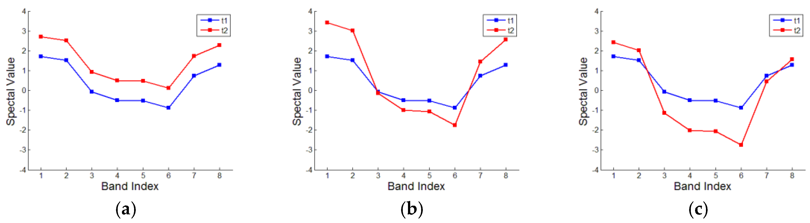
2.2. Change Detection Based on Spectral Value (CDSV) and Change Detection Based on Spectral Shapes (CDSS) Algorithms
2.2.1. CDSV Algorithm
2.2.2. CDSS Algorithm
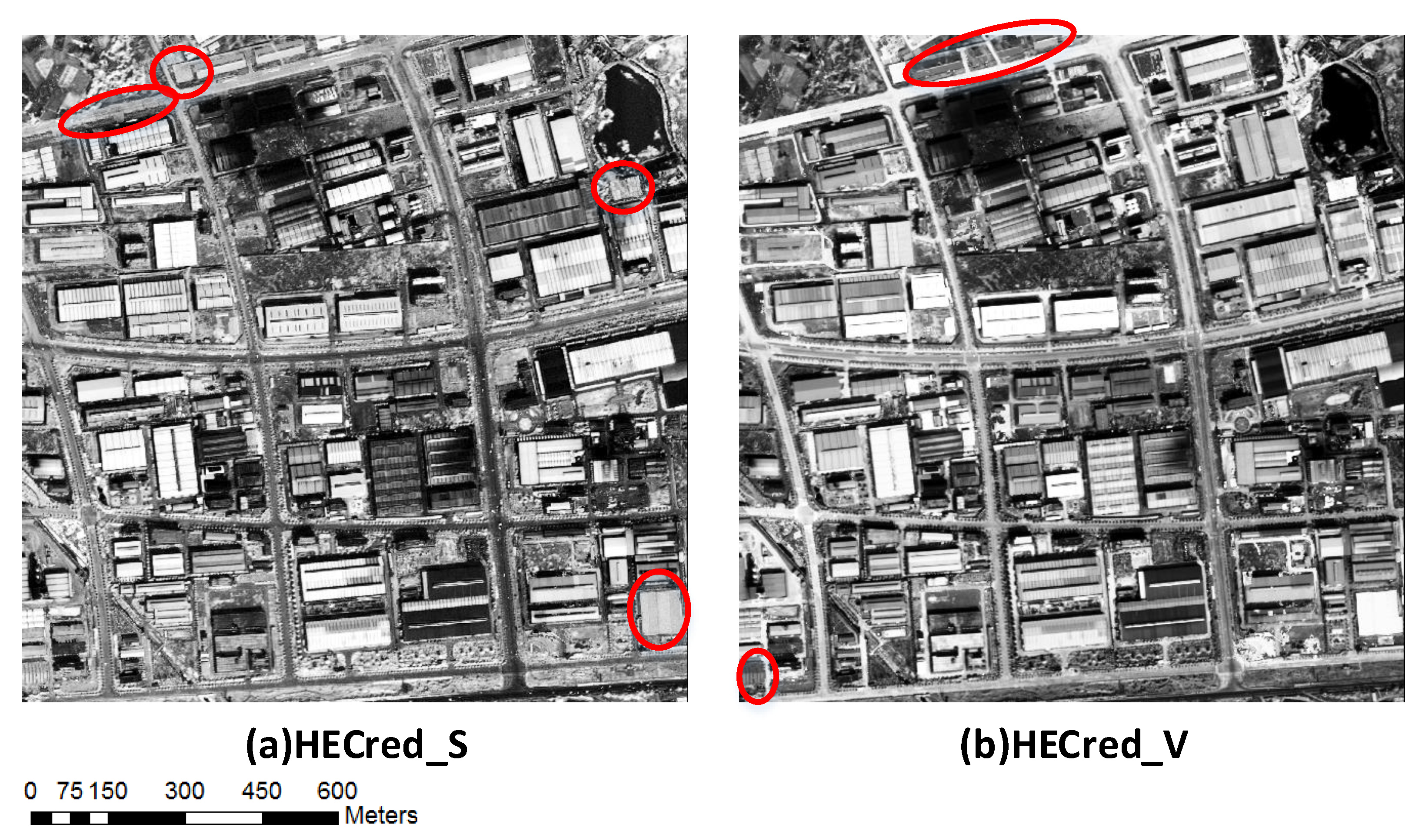
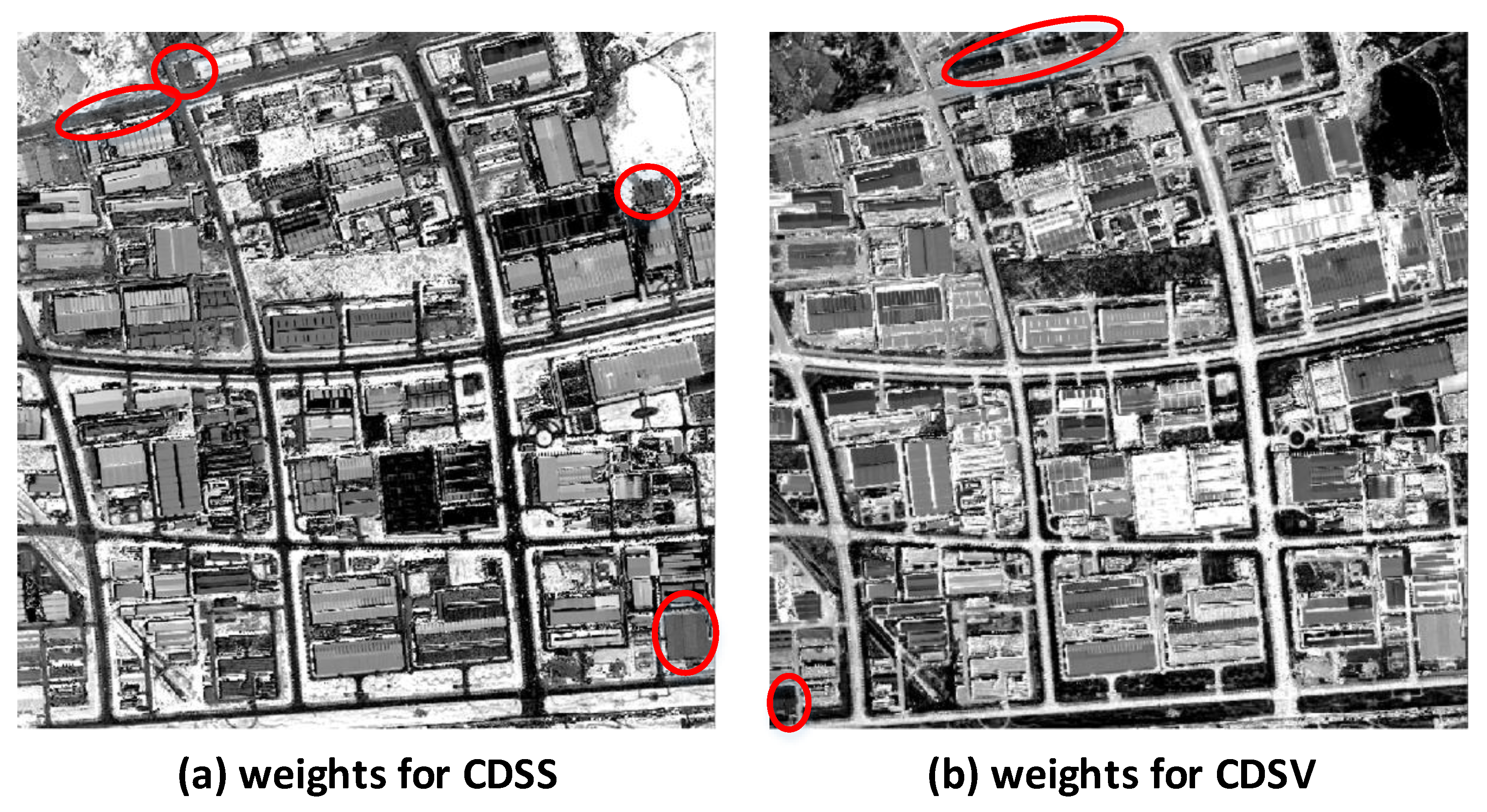
2.3. The Credibility of CDSV and CDSS
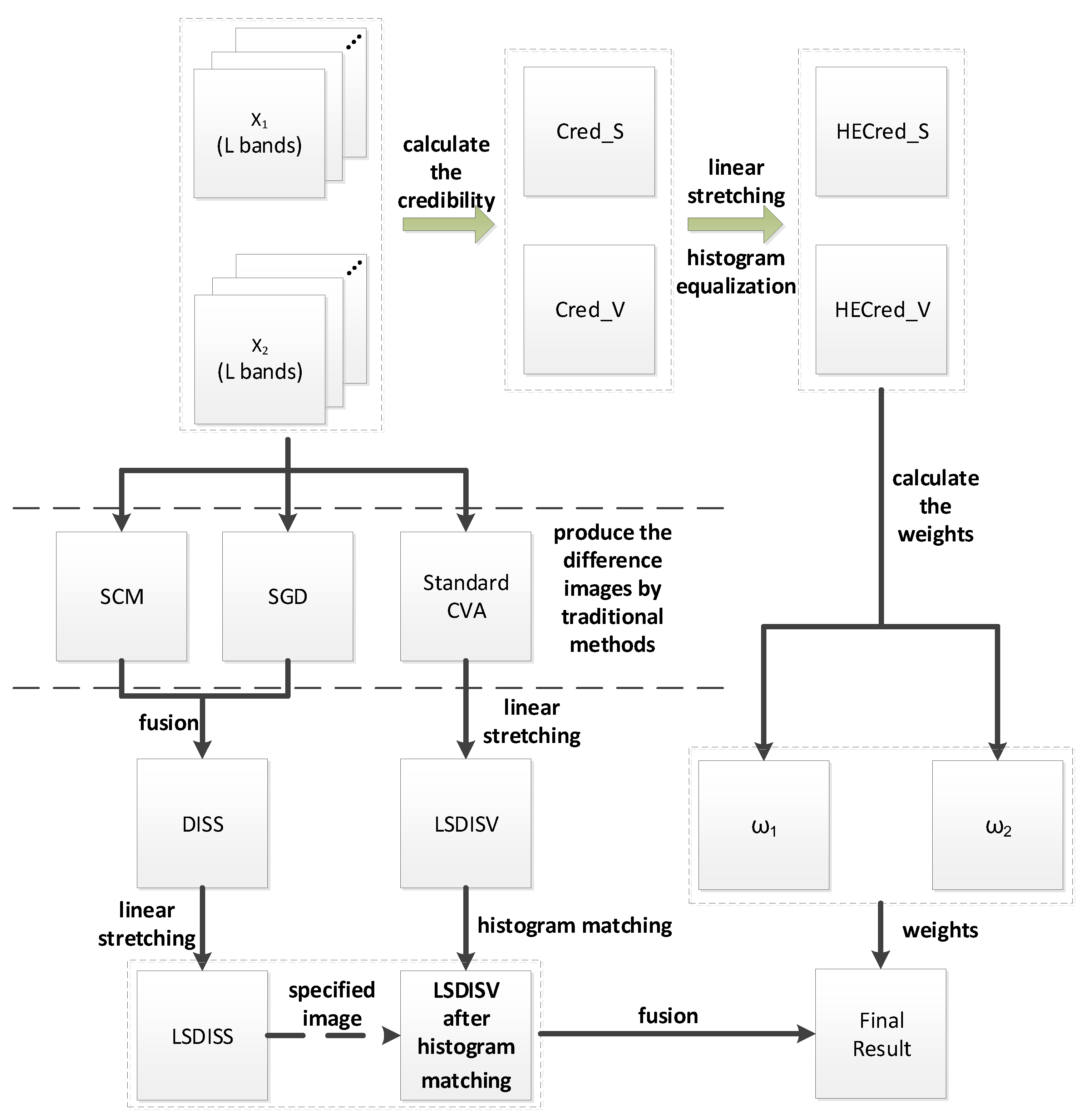
2.4. The Hybrid Spectral Difference (HSD) Algorithm
- Apply the histogram equalization transformation to two images.
- Apply the histogram matching transformation to one image and make it have the similar histogram as the other one.
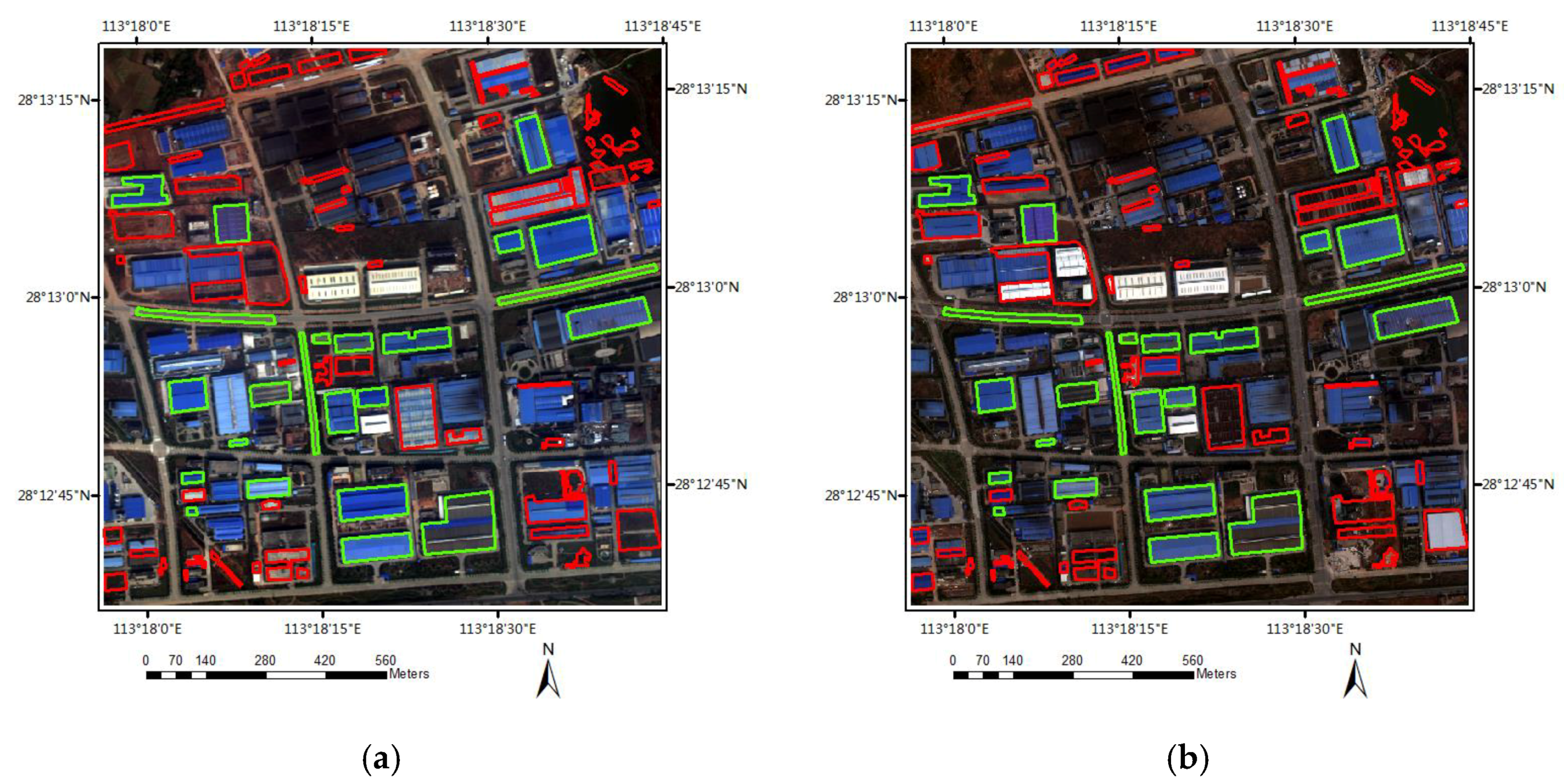
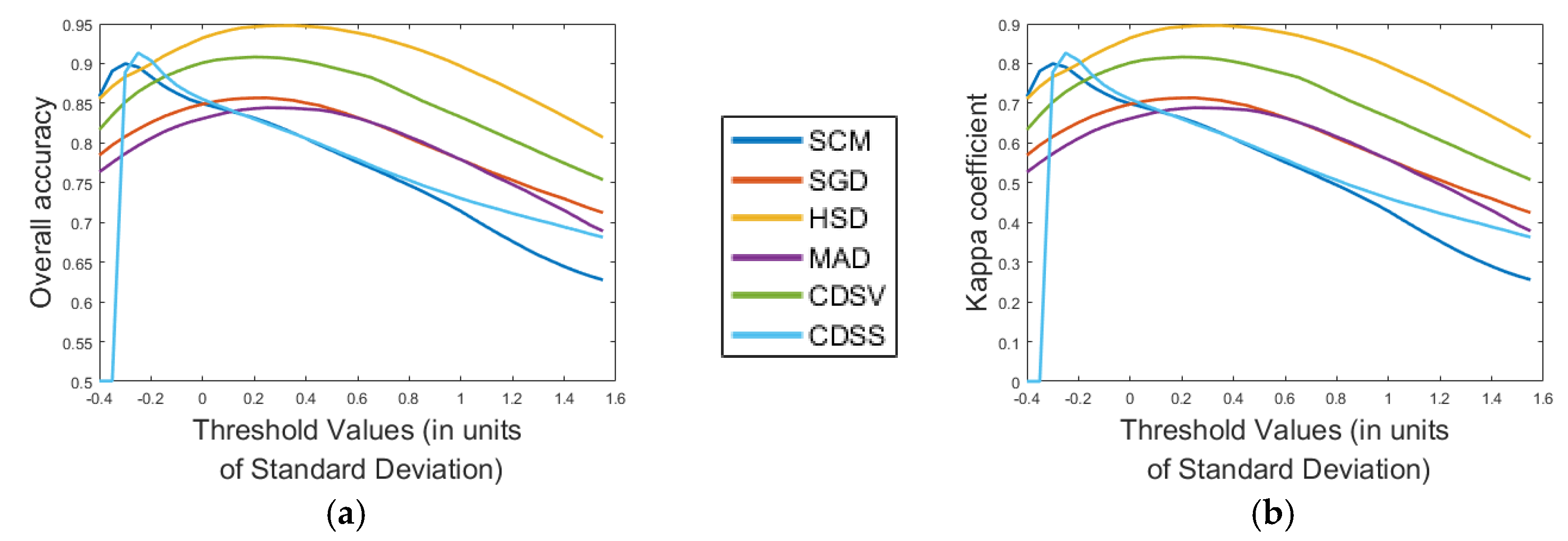
2.5. Accuracy Assessment and Reference Map
3. Experiments and Results
3.1. Case-1: Change Detection Using Worldview-2/3 Very High-Resolution (VHR) Multispectral Images
3.1.1. Material
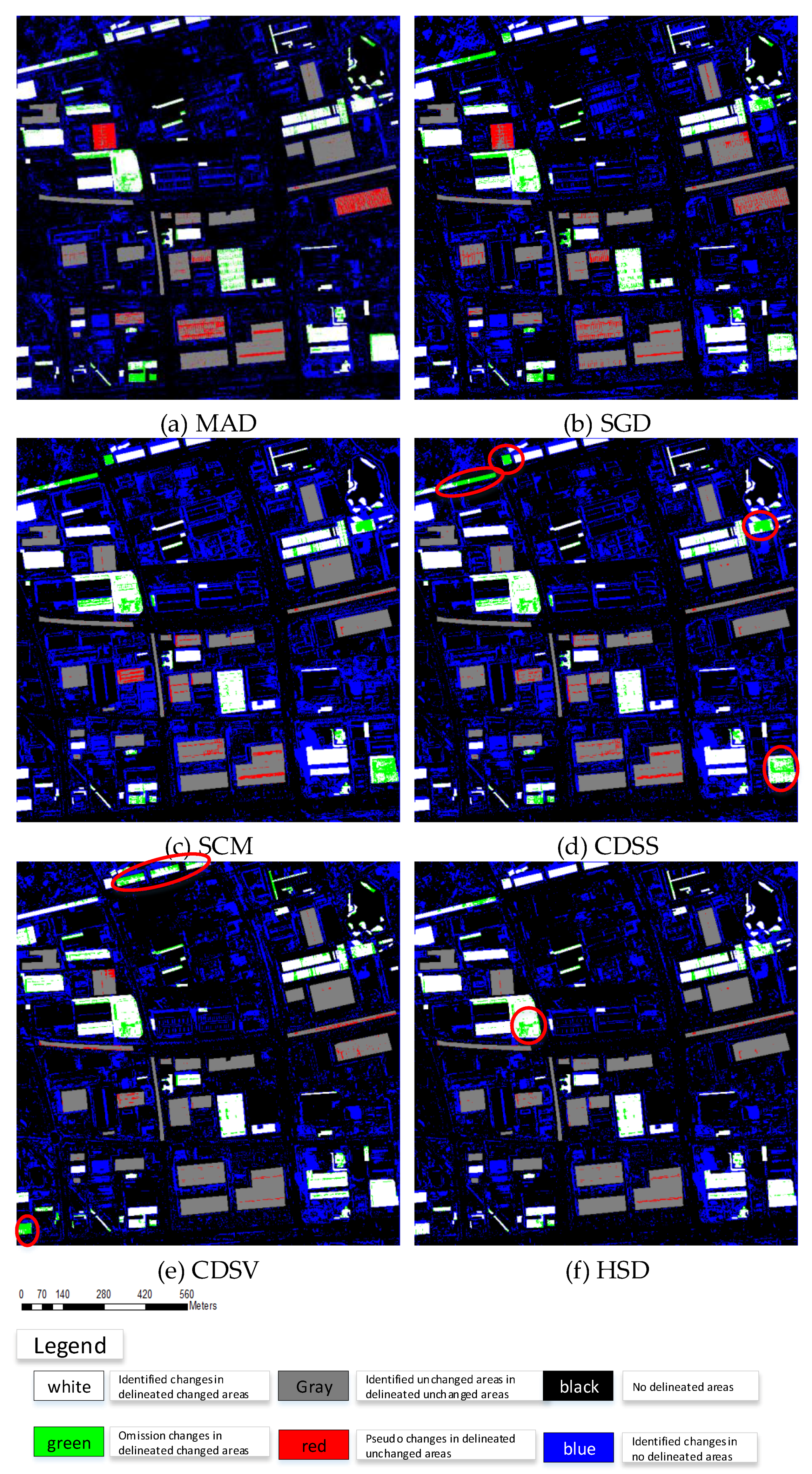
3.1.2. Results
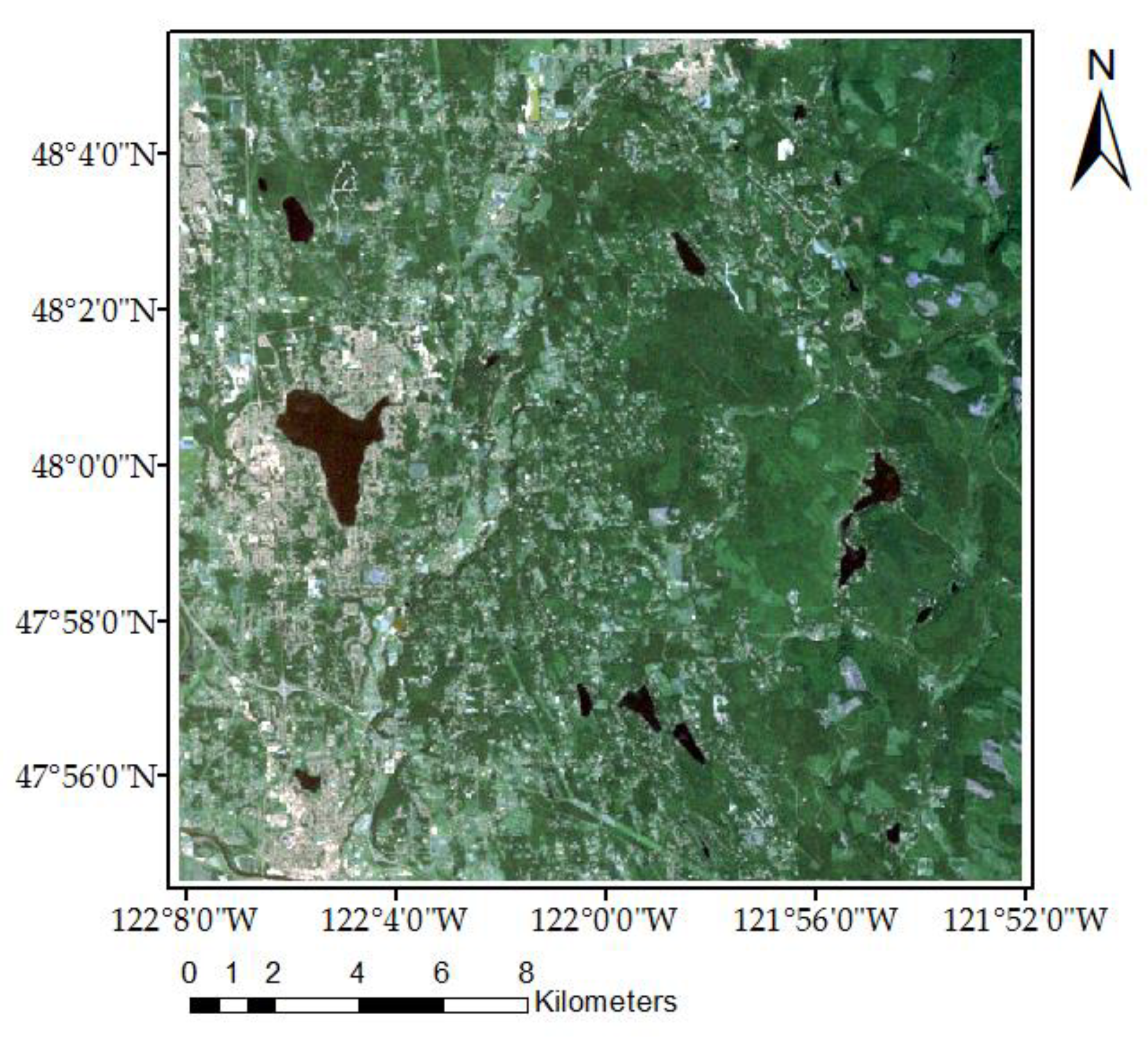
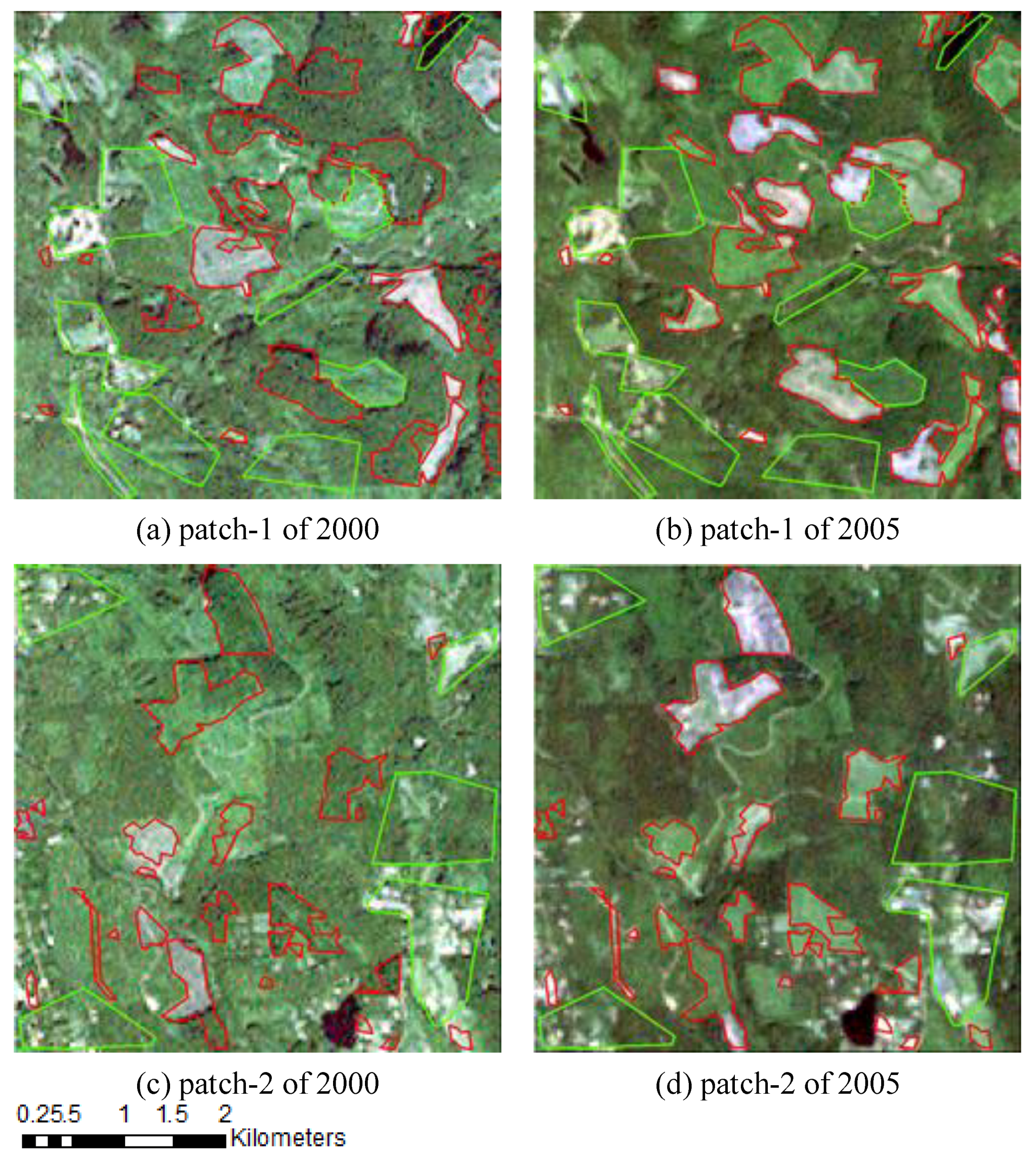
3.2. Case-2: Change Detection Using Landsat-7 Multispectral Images
3.2.1. Material and Preprocessing
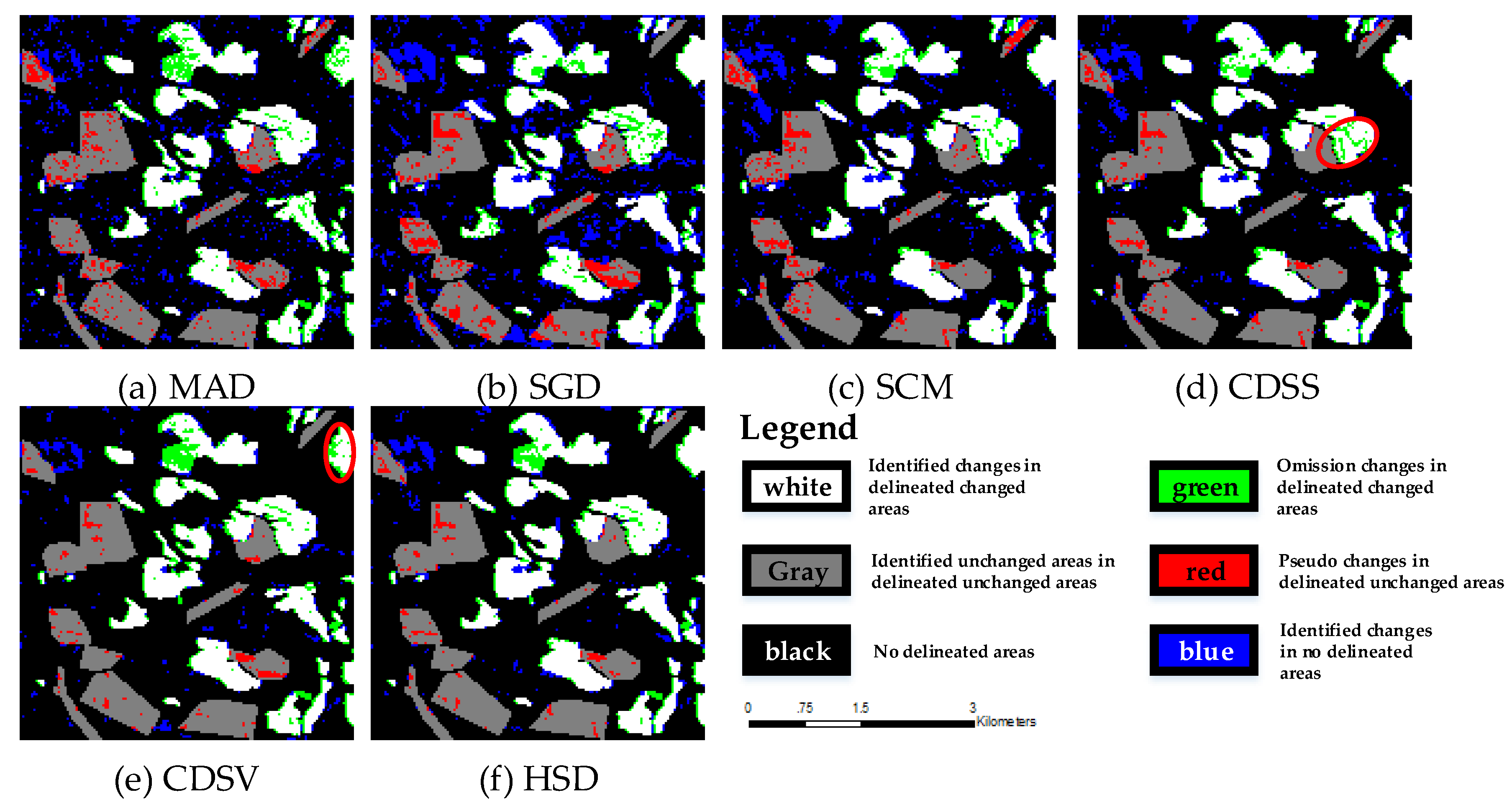
3.2.2. Results
4. Discussion
4.1. Limitation of Traditional Methods
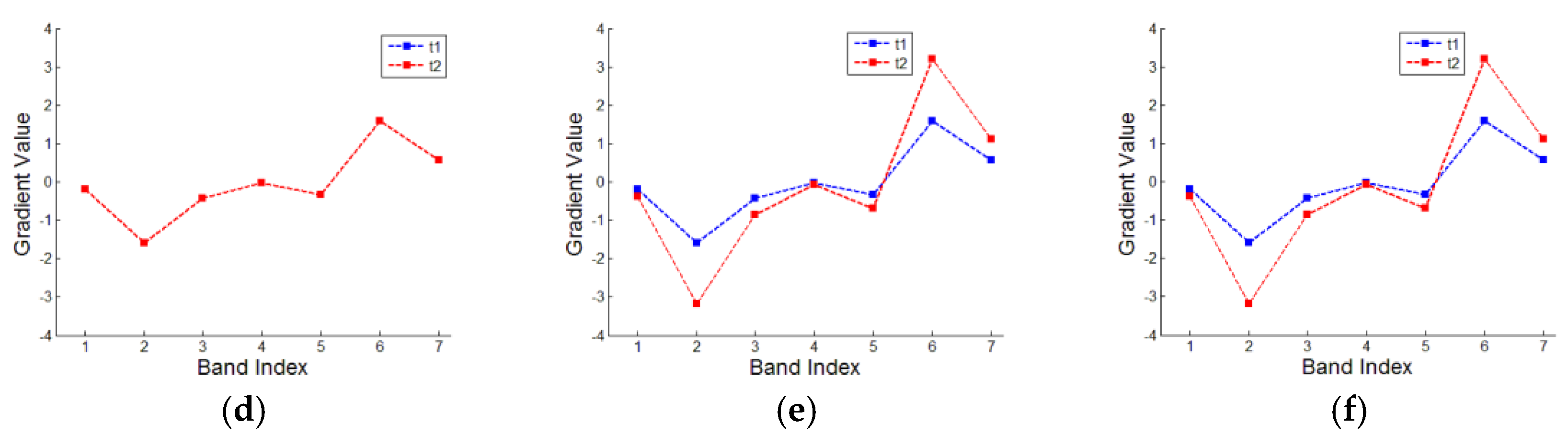
4.2. Discussion of CDSS
4.3. Superiority and Limitation of HSD
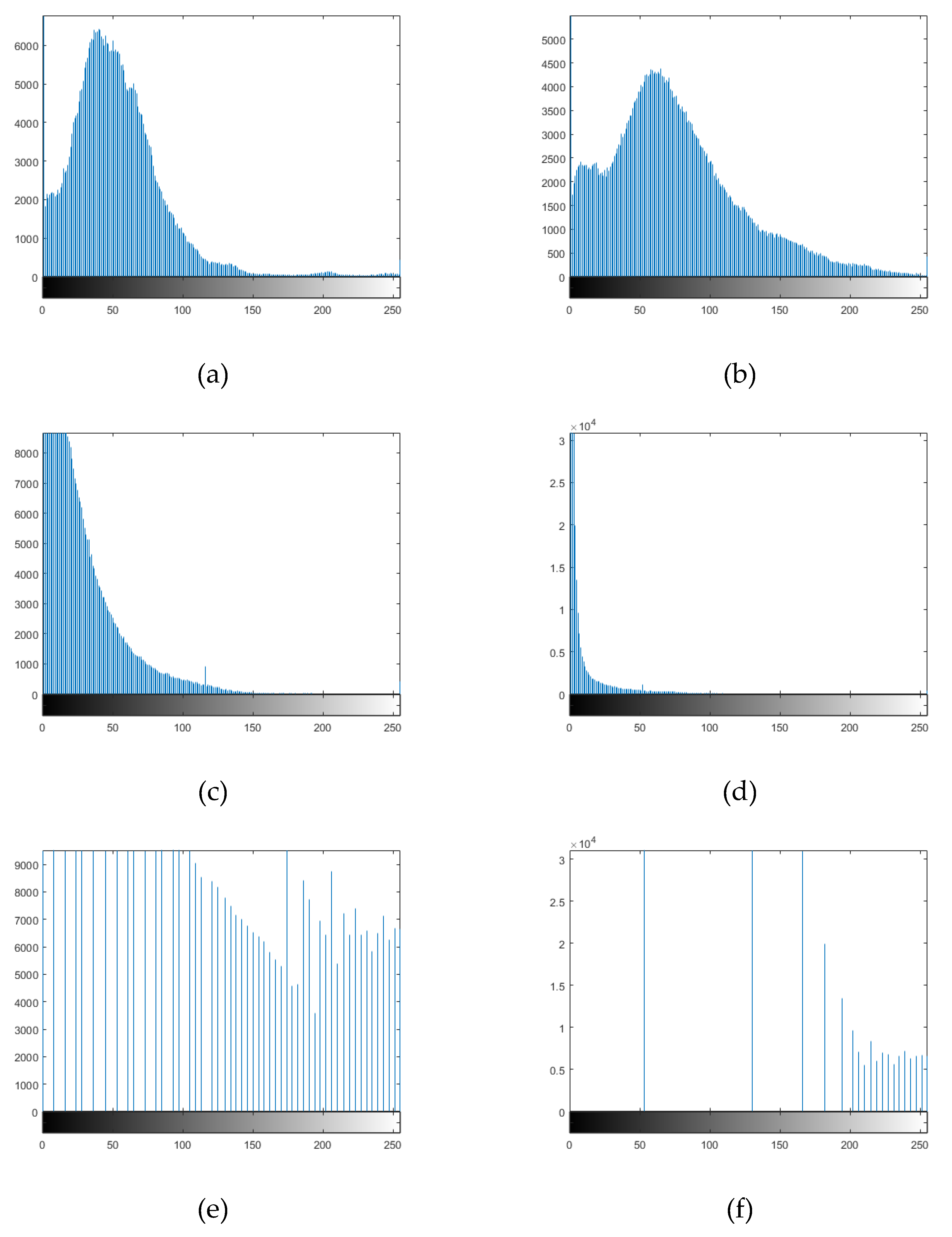
4.4. Discussion of Histogram Processing
5. Conclusions
Author Contributions
Acknowledgments
Conflicts of Interest
Abbreviations
| SCM | Spectral Correlation Mapper |
| SGD | Spectral Gradient Difference |
| CDSS | Change Detection based on Spectral Shapes, which is the fusion of SCM and SGD |
| DISS | Difference Image produced by CDSS |
| LSDISS | DISS after Linear Stretching |
| CVA | Change Vector Analysis |
| CDSV | Change Detection based on Spectral Values, which is standard CVA in this paper |
| DISV | Difference Image produced by CDSV |
| LSDISV | after Linear Stretching |
| HMLSDISV | after Histogram Matching Transformation |
| Cred_S | Credibility Of CDSS |
| Cred_V | Credibility Of CDSV |
| HECred_S | Cred_S after Histogram Equalization |
| HECred_V | Cred_V after Histogram Equalization |
| HSD | Hybrid Spectral Difference |
| DIHSD | Difference Image produced by HSD |
| MAD | Multivariate Alteration Detection |
| PIFs | Pseudo-Invariant Features |
References
- Coppin, P.; Jonckheere, I.; Nackaerts, K.; Muys, B.; Lambin, E. Digital change detection methods in ecosystem monitoring: A review. Int. J. Remote Sens. 2004, 25, 1565–1596. [Google Scholar] [CrossRef]
- Lu, D.; Mausel, P.; Brondizio, E.; Moran, E. Change detection techniques. Int. J. Remote Sens. 2004, 25, 2365–2407. [Google Scholar] [CrossRef]
- Radke, R.J.; Andra, S.; Al-Kofahi, O.; Roysam, B. Image change detection algorithms: A systematic survey. IEEE Trans. Image Process. 2005, 14, 294–307. [Google Scholar] [CrossRef] [PubMed]
- Tewkesbury, A.P.; Comber, A.J.; Tate, N.J.; Lamb, A.; Fisher, P.F. A critical synthesis of remotely sensed optical image change detection techniques. Remote Sens. Environ. 2015, 160, 1–14. [Google Scholar] [CrossRef]
- Jude, L.A.; Suruliandi, A. Performance evaluation of land cover change detection algorithms using remotely sensed data. In Proceedings of the International Conference on Circuit, Power and Computing Technologies, Nagercoil, India, 20–21 March 2015; pp. 1409–1415. [Google Scholar]
- Pons, X. Post-classification change detection with data from different sensors: Some accuracy considerations. Int. J. Remote Sens. 2003, 24, 4975–4976. [Google Scholar]
- Shao, P.; Shi, W.; He, P.; Hao, M.; Zhang, X. Novel approach to unsupervised change detection based on a robust semi-supervised FCM clustering algorithm. Remote Sens. 2016, 8, 264. [Google Scholar] [CrossRef]
- Alkhudhairy, D.H.A.; Caravaggi, I.; Giada, S. Structural damage assessments from IKONOS data using change detection, object-oriented segmentation, and classification techniques. Photogramm. Eng. Remote Sens. 2005, 71, 825–838. [Google Scholar] [CrossRef]
- Johnson, R.D.; Kasischke, E.S. Change vector analysis: A technique for the multispectral monitoring of land cover and condition. Int. J. Remote Sens. 1998, 19, 411–426. [Google Scholar] [CrossRef]
- Li, L.; Li, X.; Zhang, Y.; Wang, L.; Ying, G. Change detection for high-resolution remote sensing imagery using object-oriented change vector analysis method. In Proceedings of the IEEE International Geoscience and Remote Sensing Symposium, Beijing, China, 10–15 July 2016; pp. 2873–2876. [Google Scholar]
- Júnior, O.A.C.; Guimarães, R.F.; Gillespie, A.R.; Silva, N.C.; Gomes, R.A.T. A new approach to change vector analysis using distance and similarity measures. Remote Sens. 2011, 3, 2473–2493. [Google Scholar] [CrossRef]
- Zhuang, H.; Deng, K.; Fan, H.; Yu, M. Strategies combining spectral angle mapper and change vector analysis to unsupervised change detection in multispectral images. IEEE Geosci. Remote Sens. Lett. 2016, 13, 681–685. [Google Scholar] [CrossRef]
- Chen, J.; Lu, M.; Chen, X.; Chen, J.; Chen, L. A spectral gradient difference based approach for land cover change detection. ISPRS J. Photogramm. 2013, 85, 1–12. [Google Scholar] [CrossRef]
- Bruzzone, L.; Prieto, D.F. An adaptive semiparametric and context-based approach to unsupervised change detection in multitemporal remote-sensing images. IEEE Trans. Image Process. 2002, 11, 452–466. [Google Scholar] [CrossRef] [PubMed]
- Gong, P. Change detection using principal component analysis and fuzzy set theory. Can. J. Remote Sens. 2014, 19, 22–29. [Google Scholar] [CrossRef]
- Wiemker, R.; Kulbach, D.; Spitzer, H.; Bienlein, J. Unsupervised robust change detection on multispectral imagery using spectral and spatial features. In Proceedings of the International Airborne Remote Sensing Conference & Exhibition, Copenhagen, Denmark, 7–10 July 1997; pp. 640–647. [Google Scholar]
- Collins, J.B.; Woodcock, C.E. An assessment of several linear change detection techniques for mapping forest mortality using multitemporal Landsat TM data. Remote Sens. Environ. 1996, 56, 66–77. [Google Scholar] [CrossRef]
- Nielsen, A.A. The regularized iteratively reweighted mad method for change detection in multi- and hyperspectral data. IEEE Trans. Image Process. 2007, 16, 463–478. [Google Scholar] [CrossRef] [PubMed]
- Patra, S.; Ghosh, S.; Ghosh, A. Histogram thresholding for unsupervised change detection of remote sensing images. Int. J. Remote Sens. 2011, 32, 6071–6089. [Google Scholar] [CrossRef]
- Canty, M.J.; Nielsen, A.A. Unsupervised classification of changes in multispectral satellite imagery. In Proceedings of the 11th SPIE International Symposium Remote Sensing, Maspalomas, Gran Canaria, Spain, 13–16 September 2004. [Google Scholar]
- Bruzzone, L.; Prieto, D.F. Automatic analysis of the difference image for unsupervised change detection. IEEE Trans. Geosci. Remote Sens. 2000, 38, 1171–1182. [Google Scholar] [CrossRef]
- Tyagi, M.; Bovolo, F.; Mehra, A.K.; Chaudhuri, S.; Bruzzone, L. A context-sensitive clustering technique based on graph-cut initialization and expectation-maximization algorithm. IEEE Geosci. Remote Sens. Lett. 2008, 5, 21–25. [Google Scholar] [CrossRef]
- Melgani, F.; Bazi, Y. Markovian fusion approach to robust unsupervised change detection in remotely sensed imagery. IEEE Geosci. Remote Sens. Lett. 2006, 3, 457–461. [Google Scholar] [CrossRef]
- Benedek, C.; Szirányi, T. Markovian framework for structural change detection with application on detecting built-in changes in airborne images. In Proceedings of the Lasted International Conference on Signal Processing, Innsbruck, Austria, 14–16 February 2007; pp. 68–73. [Google Scholar]
- Chen, K.; Zhou, Z.; Lu, H.; Huo, C. Change detection based on conditional random field models. J. Southwest China Norm. Univ. 2006, 31, 111–114. [Google Scholar]
- Celik, T. Unsupervised Change Detection in Satellite Images Using Principal Component Analysis and k-Means Clustering. IEEE Geosci. Remote Sens. Lett. 2009, 6, 772–776. [Google Scholar]
- Ridd, M.K.; Liu, J. A comparison of four algorithms for change detection in an urban environment. Remote Sens. Environ. 1998, 63, 95–100. [Google Scholar] [CrossRef]
- De Carvalho, O.A.; Meneses, P.R. Spectral correlation mapper (SCM): An improvement on the spectral angle mapper (SAM). In Proceedings of the 9th Airborne Earth Science Workshop, Pasadena, CA, USA, 23–25 February 2000. [Google Scholar]
- Robila, S.A.; Gershman, A. Spectral matching accuracy in processing hyperspectral data. In Proceedings of the International Symposium on Signals, Circuits and Systems, Iasi, Romania, 14–15 July 2005; Volume 161, pp. 163–166. [Google Scholar]
- Lin, C.; Wu, C.C.; Tsogt, K.; Ouyang, Y.C.; Chang, C.I. Effects of atmospheric correction and pansharpening on LULC classification accuracy using worldview-2 imagery. Inf. Process. Agric. 2015, 2, 25–36. [Google Scholar] [CrossRef]
- Song, C.; Woodcock, C.E.; Seto, K.C.; Lenney, M.P.; Macomber, S.A. Classification and change detection using Landsat TM data: When and how to correct atmospheric effects? Remote Sens. Environ. 2001, 75, 230–244. [Google Scholar] [CrossRef]
- Zhang, L.; Wu, C.; Du, B. Automatic radiometric normalization for multitemporal remote sensing imagery with iterative slow feature analysis. IEEE Trans. Geosci. Remote Sens. 2014, 52, 6141–6155. [Google Scholar] [CrossRef]
- Zhou, H.; Liu, S.; He, J.; Wen, Q.; Song, L.; Ma, Y. A new model for the automatic relative radiometric normalization of multiple images with pseudo-invariant features. Int. J. Remote Sens. 2016, 37, 4554–4573. [Google Scholar] [CrossRef]
- Barazzetti, L.; Gianinetto, M.; Scaioni, M. Radiometric normalization with multi-image pseudo-invariant features. In Proceedings of the International Conference on Remote Sensing and Geoinformation of Environment, Paphos, Cyprus, 4–8 April 2016. [Google Scholar]
- Gonzalez, R.C.; Woods, R.E. Digital image processing. Prentice Hall Int. 1977, 28, 484–486. [Google Scholar]
- Foody, G.M. Assessing the accuracy of land cover change with imperfect ground reference data. Remote Sens. Environ. 2010, 114, 2271–2285. [Google Scholar] [CrossRef]
- Foody, G.M. The impact of imperfect ground reference data on the accuracy of land cover change estimation. Int. J. Remote Sens. 2009, 30, 3275–3281. [Google Scholar] [CrossRef]
- Ma, L.; Li, M.; Blaschke, T.; Ma, X.; Tiede, D.; Cheng, L.; Chen, Z.; Chen, D. Object-based change detection in urban areas: The effects of segmentation strategy, scale, and feature space on unsupervised methods. Remote Sens. 2016, 8, 761. [Google Scholar] [CrossRef]
- Sinha, P.; Kumar, L. Independent two-step thresholding of binary images in inter-annual land cover change/no-change identification. ISPRS J. Photogramm. Remote Sens. 2013, 81, 31–43. [Google Scholar] [CrossRef]
- Pontius, R.G., Jr.; Millones, M. Death to kappa: Birth of quantity disagreement and allocation disagreement for accuracy assessment. Int. J. Remote Sens. 2011, 32, 4407–4429. [Google Scholar] [CrossRef]
- Stein, A.; Aryal, J.; Gort, G. Use of the Bradley-Terry model to quantify association in remotely sensed images. IEEE Trans. Geosci. Remote Sens. 2005, 43, 852–856. [Google Scholar] [CrossRef]
- FLAASH Module. Atmospheric Correction Module: QUAC and FLAASH User’s Guide, version 4.7; ITT Visual Information Solutions: Boulder, CO, USA, 2009. [Google Scholar]
- Zanotta, D.C.; Haertel, V. Gradual land cover change detection based on multitemporal fraction images. Pattern Recognit. 2012, 45, 2927–2937. [Google Scholar] [CrossRef]
- Löw, F.; Michel, U.; Dech, S.; Conrad, C. Impact of feature selection on the accuracy and spatial uncertainty of per-field crop classification using support vector machines. ISPRS J. Photogramm. Remote Sens. 2013, 85, 102–119. [Google Scholar] [CrossRef]
- Anees, A.; Aryal, J.; O’Reilly, M.M.; Gale, T.J.; Wardlaw, T. A robust multi-kernel change detection framework for detecting leaf beetle defoliation using Landsat 7 ETM+ data. ISPRS J. Photogramm. Remote Sens. 2016, 122, 167–178. [Google Scholar] [CrossRef]
- Symeonakis, E.; Higginbottom, T.; Petroulaki, K.; Rabe, A. Optimisation of savannah land cover characterisation with optical and SAR data. Remote Sens. 2018, 10, 499. [Google Scholar] [CrossRef]
- Lin, H.; Song, S.; Yang, J. Ship classification based on MSHOG feature and task-driven dictionary learning with structured incoherent constraints in SAR images. Remote Sens. 2018, 10, 190. [Google Scholar] [CrossRef]
- Cheng, G.; Han, J. A survey on object detection in optical remote sensing images. ISPRS J. Photogramm. Remote Sens. 2016, 117, 11–28. [Google Scholar] [CrossRef]
- Zhong, Y.; Huang, R.; Zhao, J.; Zhao, B.; Liu, T. Aurora image classification based on multi-feature latent dirichlet allocation. Remote Sens. 2018, 10, 233. [Google Scholar] [CrossRef]


| Image | Acquired Time | Resolution | Product Level | Off Nadir View Angle | Area | Number of Bands |
|---|---|---|---|---|---|---|
| Worldview-2 | 2011-11-23 | 2 m | 2A | 18.4° | 1.3 km × 1.3 km | 8 |
| Worldview-3 | 2015-02-09 | 1.2 m | 2A | 23.7° | 1.3 km × 1.3 km | 8 |
| Algorithm | Overall Accuracy | Kappa Coefficient | Omission Rate | Commission Rate |
|---|---|---|---|---|
| Multivariate alteration detection (MAD) | 0.8442 | 0.6883 | 0.1037 | 0.208 |
| Spectral gradient difference (SGD) | 0.8568 | 0.7137 | 0.1344 | 0.152 |
| Spectral correlation mapper (SCM) | 0.8998 | 0.7996 | 0.0874 | 0.113 |
| Change detection based on spectral shapes (CDSS) | 0.9133 | 0.8265 | 0.09747 | 0.07603 |
| Change detection based on spectral values (CDSV) | 0.9082 | 0.8164 | 0.1105 | 0.07303 |
| Hybrid spectral difference (HSD) | 0.9478 | 0.8957 | 0.05342 | 0.05085 |
| Algorithm | Overall Accuracy | Kappa Coefficient | Omission Rate | Commission Rate |
|---|---|---|---|---|
| MAD | 0.8306 | 0.6612 | 0.1874 | 0.1512 |
| SCM | 0.8523 | 0.7046 | 0.1417 | 0.1538 |
| SGD | 0.8286 | 0.657 | 0.1393 | 0.2039 |
| CDSS | 0.8665 | 0.7332 | 0.1629 | 0.1037 |
| CDSV | 0.8725 | 0.7452 | 0.1911 | 0.06312 |
| HSD | 0.8891 | 0.7783 | 0.1467 | 0.07466 |
| Image | Statistics | SGD | SCM | CDSS | Delineated Change |
|---|---|---|---|---|---|
| Case-1 | mean | 60 | 95 | 88 | 110 |
| std | 31 | 28 | 28 | 44 | |
| Patch-1 in case-2 | mean | 109 | 127 | 123 | 142 |
| std | 39 | 46 | 47 | 46 | |
| Patch-2 in case-2 | mean | 128 | 143 | 124 | 159 |
| std | 37 | 31 | 57 | 34 |
| Image | Statistics | CDSV | Delineated Change |
|---|---|---|---|
| Case-1 | mean | 44 | 90 |
| std | 19 | 50 | |
| Patch-1 in case-2 | mean | 93 | 116 |
| std | 48 | 40 | |
| Patch-2 in case-2 | mean | 100 | 124 |
| std | 32 | 32 |
© 2018 by the authors. Licensee MDPI, Basel, Switzerland. This article is an open access article distributed under the terms and conditions of the Creative Commons Attribution (CC BY) license (http://creativecommons.org/licenses/by/4.0/).
Share and Cite
Yan, L.; Xia, W.; Zhao, Z.; Wang, Y. A Novel Approach to Unsupervised Change Detection Based on Hybrid Spectral Difference. Remote Sens. 2018, 10, 841. https://doi.org/10.3390/rs10060841
Yan L, Xia W, Zhao Z, Wang Y. A Novel Approach to Unsupervised Change Detection Based on Hybrid Spectral Difference. Remote Sensing. 2018; 10(6):841. https://doi.org/10.3390/rs10060841
Chicago/Turabian StyleYan, Li, Wang Xia, Zhan Zhao, and Yanran Wang. 2018. "A Novel Approach to Unsupervised Change Detection Based on Hybrid Spectral Difference" Remote Sensing 10, no. 6: 841. https://doi.org/10.3390/rs10060841
APA StyleYan, L., Xia, W., Zhao, Z., & Wang, Y. (2018). A Novel Approach to Unsupervised Change Detection Based on Hybrid Spectral Difference. Remote Sensing, 10(6), 841. https://doi.org/10.3390/rs10060841