Article

Application of Thermal and Phenological Land Surface Parameters for Improving Ecological Niche Models of Betula utilis in the Himalayan Region

1
Center for Earth System Research and Sustainability, Institute of Geography, University of Hamburg, Bundesstraße 55, 20146 Hamburg, Germany
2
Biodiversity, Evolution and Ecology of Plants (BEE), Biocenter Klein Flottbek and Botanical Garden, University of Hamburg, Ohnhorststr. 18, 22609 Hamburg, Germany
*
Author to whom correspondence should be addressed.
Remote Sens. 2018, 10(6), 814; https://doi.org/10.3390/rs10060814
Submission received: 24 April 2018 / Revised: 18 May 2018 / Accepted: 22 May 2018 / Published: 24 May 2018

Abstract

:
Modelling ecological niches across vast distribution ranges in remote, high mountain regions like the Himalayas faces several data limitations, in particular nonavailability of species occurrence data and fine-scale environmental information of sufficiently high quality. Remotely sensed data provide key advantages such as frequent, complete, and long-term observations of land surface parameters with full spatial coverage. The objective of this study is to evaluate modelled climate data as well as remotely sensed data for modelling the ecological niche of Betula utilis in the subalpine and alpine belts of the Himalayan region covering the entire Himalayan arc. Using generalized linear models (GLM), we aim at testing factors controlling the species distribution under current climate conditions. We evaluate the additional predictive capacity of remotely sensed variables, namely remotely sensed topography and vegetation phenology data (phenological traits), as well as the capability to substitute bioclimatic variables from downscaled numerical models by remotely sensed annual land surface temperature parameters. The best performing model utilized bioclimatic variables, topography, and phenological traits, and explained over 69% of variance, while models exclusively based on remotely sensed data reached 65% of explained variance. In summary, models based on bioclimatic variables and topography combined with phenological traits led to a refined prediction of the current niche of B. utilis, whereas models using solely climate data consistently resulted in overpredictions. Our results suggest that remotely sensed phenological traits can be applied beneficially as supplements to improve model accuracy and to refine the prediction of the species niche. We conclude that the combination of remotely sensed land surface temperature parameters is promising, in particular in regions where sufficient fine-scale climate data are not available.

Graphical Abstract

1. Introduction

As high-elevation treelines can be considered indicators of past and recent climate change and variability [1,2], ecological niche modelling studies frequently use climate variables from numerical models to predict the current and future potential distribution of treeline species [3,4,5]. However, these predictions potentially disregard important local abiotic or biotic factors, which influence the actual species’ distribution (i.e., the realized niche) because climate is not the exclusive factor determining habitat suitability [6]. To date, the number of studies modelling distribution ranges of deciduous treeline species’ in the entire Himalayan mountains remains very limited (e.g., [7,8]). Studies which evaluate the performance of ecological niche models comparing many different predictor sets for modelling the current distribution of a treeline species covering the entire Himalayan arc do not exist. As pointed out by Bobrowski and Schickhoff [9], modelling species’ distributions in high-altitude regions faces numerous challenges, most importantly the sparse data availability due to poor accessibility of the terrain. This applies in particular to species occurrence data (often obtained from herbaria) as well as to environmental predictors such as climate variables, which are often spatially interpolated and afflicted with errors [9].
Therefore, remotely sensed data can provide additional, spatially contiguous information in higher resolution and accuracy in particular in remote areas like the Himalayan mountains, giving insight into vegetation characteristics and spatial patterns, surface temperatures, and topographical features. Since the availability of multispectral satellite images in the early 1970s, biophysical mapping of the earth’s surface has contributed to ecological studies [10,11,12]. Previous studies have documented the merit of incorporating remote sensing data in species distribution models such as land cover data [13,14,15] and topographical information from the Shuttle Radar Topography Mission (SRTM) (for examples, see [16]). Today, remote sensing data play an increasing role in modelling species distributions [17,18,19,20]. Compared to models using solely climatic/topographical predictors [18,21,22,23], the inclusion of remotely sensed variables as predictors in species distribution models improves prediction accuracy and refines the mapped distribution range of the species. The spectral measurements and their derivates are directly linked to biophysical properties of the land surface which, in turn, are linked to the primary environmental regimes and to habitat quality (productivity, vegetation structure, land cover type) [24]. Thus, the use of remotely sensed variables may also help to improve the understanding of the interactions of driving factors for complex species composition and vegetation zonation, e.g., at alpine treelines. This includes phenological traits, which represent species characteristics of recurring seasonal biological events in the life cycles [25,26]. Remote-sensing-based phenological analyses yielded notable results for modelling species’ distributions [27,28,29].
For this study in the Himalayan mountains, characterized by distinct vertical climatic gradients and respective altitudinal zonations of vegetation, we selected the treeline-forming Himalayan Birch (Betula utilis) as a target species. Birch forests feature prominently within this zonation, and B. utilis constitutes an ideal study organism due to its status as a principal deciduous broadleaved treeline species. The distribution extends across the Himalayan arc with higher dominance in the western and central part of the mountain system. Over much of its range, B. utilis forms a narrow forest belt on north-facing slopes between evergreen coniferous forests (e.g., Abies spectabilis) below and an evergreen broadleaved krummholz belt (e.g., Rhododendron campanulatum) above (for more associated tree species, see [30,31]).
Bobrowski et al. [32] and Bobrowski and Schickhoff [9] modelled the potential distribution of B. utilis at a smaller spatial extent in the Himalayan region using modelled climate-related predictor variables only. In this study, we aim to bridge the gap between species’ potential and actual distributions by deriving the first comprehensive ecological niche models for B. utilis for the entire Himalayan mountains, as well as by supplementing and substituting the standard predictors with remotely sensed land surface temperature, vegetation phenology, and topography parameters. In particular, we investigate the suitability of various predictor sets including bioclimatic variables (Chelsa [33]), topography [34], phenological traits derived from MODIS Land Cover Dynamics data [35], annual cycle parameters derived from MODIS Land Surface Temperature data [36], and their combinations. In light of the above, we (1) analyse possibilities to improve the niche model of B. utilis based solely on bioclimatic variables by adding different remotely sensed variables, and (2) explore the potential of a pure remote sensing approach by substituting the bioclimatic variables with remotely sensed land surface temperature data.

2. Materials and Methods

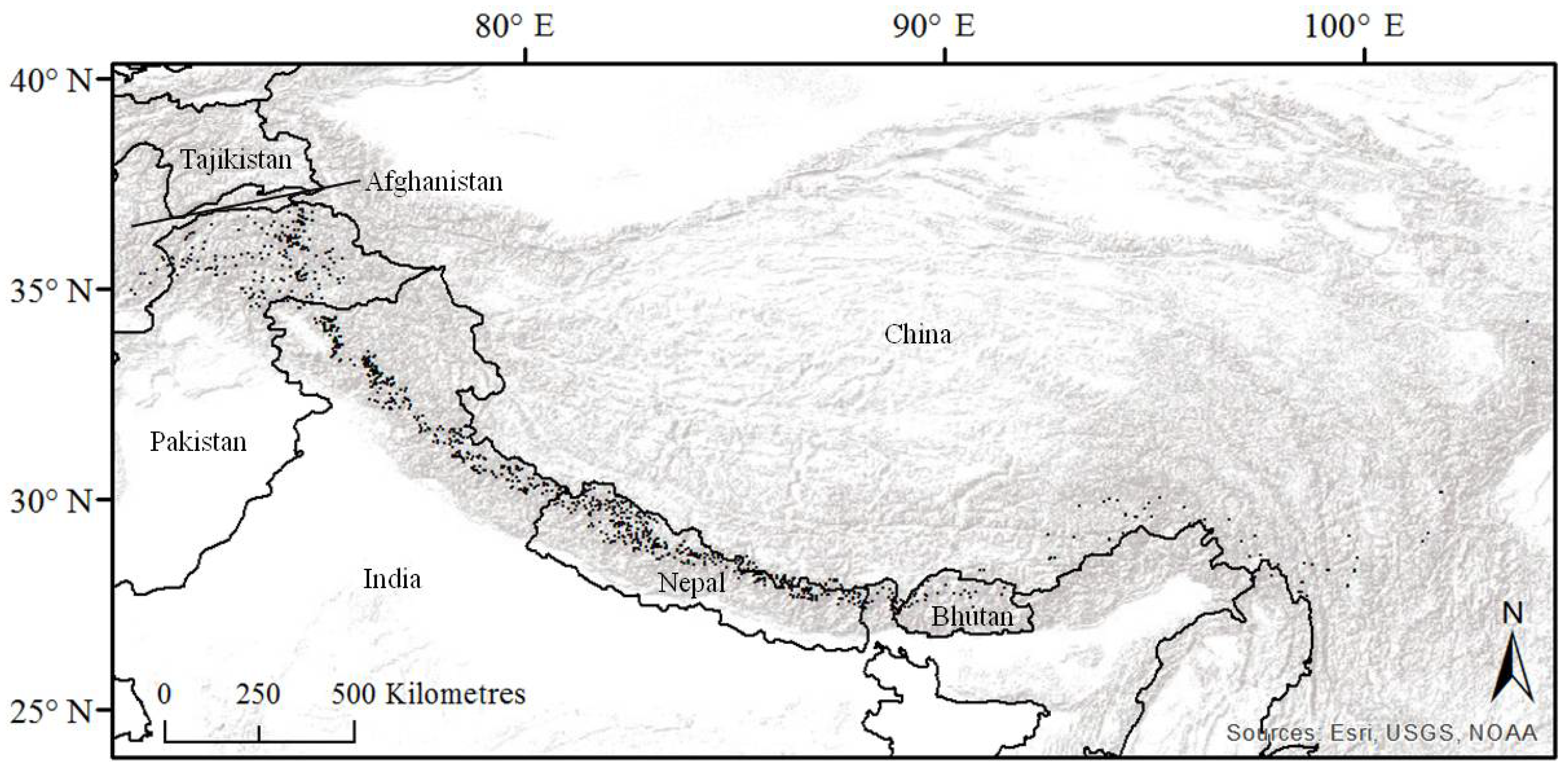
2.1. Study Area and Species Data

The Himalayan mountains are located between the Indian Subcontinent in the south and the Tibetan Highland in the north, extending from Afghanistan in the northwest (c. 36°N and 70°E) to Yunnan in the southeast (c. 26°N and 100°E), and covering an area of more than 1,000,000 km2. Due to a distinct three-dimensional geoecological differentiation, the Himalayas show a high variation of climate, rainfall, altitude, and soils [37,38]. The climate ranges from tropical in the Indian lowlands to permanent ice and snow at the highest elevations, and from more continental in the northwest to more oceanic in the southeast [39].
The distribution range of B. utilis extends across the Himalayan arc from Afghanistan to southwest China. Towards the eastern Himalayas, where more maritime climatic conditions favour the competitiveness of evergreen Rhododendron spp., B. utilis becomes a less frequent companion in subalpine forests and at treelines [30]. The total elevational range of B. utilis extends from 2700 to 4500 m [40]. In the northwest Himalayas, B. utilis is widely distributed between 3100 and 3700 m, while the range shifts to higher elevations towards the eastern Himalayas (mainly between 3800 and 4300 m). Pure birch stands with Rhododendron campanulatum and Sorbus microphylla in the understory and are often found at the uppermost limit of subalpine forests [41].
Presence-only occurrence data of B. utilis were compiled from three different sources: 215 geo-referenced records (1980–2016) were accessed via the Global Biodiversity Information Facility [42]. Further, 202 records were added from a database compiled from a literature survey ([30], unpublished data). Additionally, 827 records were extracted from freely available satellite images (GoogleEarthTM [43]) and added to the dataset. Extractions from GoogleEarth have been shown to be valuable in global treeline research [44,45]. These occurrence localities were validated through expert knowledge, obtained from numerous field visits in the Himalayan mountains.
Lowermost occurrences (e.g., in avalanche paths) were removed since they do not represent the “zonal” climatic conditions of the treeline birch belt. To reduce spatial autocorrelation, we kept only one occurrence point per grid cell (i.e., 1 km × 1 km), resulting in 1041 occurrence points for modelling the current distribution of B. utilis (Figure 1).

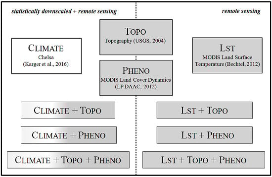
2.2. Predictor Variable Sets

The aim of the study was to evaluate the performance of four different predictor variable sets: (1) a quasi-mechanistical statistically downscaled Chelsa Climate data set [33]; (2) topographical variables based on a remotely sensed Digital Elevation Model (Topo) [34]; (3) phenological traits derived from MODIS Land Cover Dynamics data (Pheno) [35]; and (4) annual cycle parameters derived from MODIS Land Surface Temperature data (Lst) [36]. Furthermore, we assessed the suitability of combinations of these predictor variable sets using an additive procedure, which resulted in 11 final models (Figure 2). First, every predictor set was used separately, followed by the combination of two and three predictor sets. Subsequently, two approaches were followed: (1) combinations of statistically downscaled variables with remotely sensed variables; and (2) combinations of exclusively remotely sensed variables.
To test the potential of surface temperature to substitute downscaled climate data, predictor sets Topo and Pheno were combined with either Climate or Lst (Figure 2).
All predictor variables were tested for multicollinearity using Spearman’s rank correlation, since high collinearity might lead to low model performance and wrong interpretations [46]. Regarding climate variables, only ecologically relevant variables were included, which represent general patterns and annual climatic variability in the Himalayan mountains. We calculated pairwise correlations, resulting in a small set of predictor variables (rs ≤ 0.7 according to [46]) (Table 1).

2.2.1. Chelsa Climate Data

Chelsa climate data (Climate) are based on quasi-mechanistical statistical downscaling of the ERA-interim global circulation model with Global Precipitation Climatology Centre and Global Historical Climatology Network bias correction, and a resolution of 30 arc seconds (for details, see [33]). Precipitation amounts, estimated under consideration of orographic factors such as wind fields, valley exposure, and boundary layer height, showed high precision compared to precipitation data from other climate data sets [33].
Based on the gridded monthly fields of temperature and precipitation at a resolution of 30 arc seconds, we generated 19 bioclimatic variables (Table 1), which are widely used in species distribution modelling and represent annual characteristics (e.g., Temperature Annual Range), seasonality (e.g., Precipitation Seasonality) and extreme environmental factors (e.g., Precipitation of Driest Month) [47]. In addition, the variables Average Precipitation of May and Average Precipitation of March, April, and May were calculated in order to account for potential premonsoon drought stress [41,48,49]. The selected bioclimatic variables have proven to be suitable for modelling the potential distribution of B. utilis at smaller spatial scales in the Himalayan mountains [32].

2.2.2. Digital Elevation Model

The topographic data is based on the Digital Elevation Model obtained by the Shuttle Radar Topography Mission (SRTM) [34], which employed interferometric synthetic aperture radar, and which is considered here as a remote sensing dataset as well. The data was aggregated to a 1 km grid to calculate Slope angle and Slope aspect using SAGA GIS [50], complementing the set of potential explanatory variables. Since Slope aspect is a circular variable, it was converted into two separate continuous quantitative variables (i.e., Northness and Eastness).

2.2.3. MODIS Land Cover Dynamics

We chose MODIS Land Cover Dynamics (Pheno) product MCD12Q2 as it provides eight parameters that can be linked to phenological events and plants’ phenology [35]. The data was obtained from the NASA Land Processes Distributed Active Archive Center [35]. We compiled time series with a spatial resolution of 500 m × 500 m from 2000 to 2013 using the 16-day composite. Long term means of the annual metrics were used to reduce the effect of the interannual variability. Four variables providing cardinal phenophase transition dates at annual time steps were selected (Onset Greenness Increase, Onset Greenness Maximum, Onset Greenness Decrease, and Onset Greenness Minimum). These dates correspond to the timing of vegetation green-up, maturity, senescence, and dormancy, respectively. Furthermore, we selected the Enhanced Vegetation Index (EVI [51]). The first two EVI metrics (EVI Onset Greenness Min and EVI Onset Greenness Max) correspond to the EVI value of green-up and dormancy onset dates. The third metric records the sum of fitted daily EVI values during the identified vegetation cycle (i.e., Onset Greenness Increase to Onset Greenness Minimum)—EVI Area. For further information on the calculation of each Pheno predictor, see Zhang et al. [52,53] and Ganguly et al. [54].

2.2.4. MODIS Land Surface Temperature

MODIS Land Surface Temperature (Lst) offers a unique archive of daily Lst observations in 1 km resolution [55]. However, Lst is a spatially and temporally highly variable quantity, and moreover affected by plenty of gaps resulting from cloud coverage. Therefore, we use long time series rather than few observations to model the long-term seasonality of Lst. A model is fitted for the annual temperature cycle resulting in parameters that describe the annual temperature variation [36,56]. Here, we use a model with three parameters, which is sufficient for regions outside the tropics [57]. MAST is the mean annual land surface temperature for 2003–2014, YAST is the mean annual amplitude of the land surface temperature for 2003–2014, and THETA is the phase shift in days relative to spring equinox on the northern hemisphere. Additionally, we used NCSA, which represents the number of clear-sky acquisitions. These parameters represent a very robust estimate of Lst and its annual dynamics but can also be used to estimate Lst for any day of the year. The parameters were derived globally based on collection 5 of the MODIS daily level 3 global 1 km grid product from EOS Terra and Aqua (MOD11A1 and MYD11A1)—separately for night time and for day time (see [36] for details on calculation). For this study, these four variables were reprojected to the target grid and directly considered as predictor variables.

2.3. Modelling Algorithm

Generalized linear models (GLM) were applied since they represent a classical and robust approach to analyse presence and absence data [58]. Major advantages of GLMs over more complex machine-learning algorithms (e.g., random forest) include predictions which are easily interpretable and not “black box” predictions. We used the iterative weighted linear regression technique to derive maximum likelihood estimates of the response variable, with observations distributed according to exponential family and systematic effects [59]. We calculated GLMs with binomial distribution, logit-link function, and polynomial terms of second order [60], but did not include interaction terms among predictor variables. Prior to the modelling, stepwise variable selection in both directions (i.e., forward and backward) was applied using the Akaike Information Criterion (AIC) [61], resulting in the model possessing the lowest AIC value [62,63] for each predictor variable set respectively.

2.4. Pseudo-Absence Selection

As GLMs need presence and absence points, pseudo-absence points were generated. For study area selection, we used a convex hull, covering the full extent of the known occurrences of B. utilis distribution in the Himalayan region. By limiting the study area, large regions where the species cannot occur were excluded in further statistical analyses in order to prevent overpredicting the distribution range of the species [64]. For random selection of pseudo-absences, the limits were set as 5 km from the nearest occurrence, resulting in total 10,000 pseudo-absences (following the pseudo-absence selection procedure for GLMs described by Barbet-Massin et al. [65]).

2.5. Model Evaluation

For model validation, all presence and pseudo-absence points were split into training and testing data samples with a ratio of 80:20 percent using random sample splitting [66]. For each predictor variable set respectively, we repeated this procedure five times, resulting in five versions of the model and accuracy metrics, which were finally averaged. Due to the lack of a universally valid model evaluation measurement, we applied several performance evaluation metrics. Calculated evaluation measures included the AIC, the Area Under the Curve (AUC), Cohen’s Kappa, and the coefficient of determination for explained variance in the data set (Pseudo-R2; [67]). We calculated the root mean square error (RMSE) in order to account for overfitting of the data (i.e., RMSE should be very similar between training and testing data sets), indicating a good fit of all models. Moreover, visual inspection on spatial patterns of the predictions was conducted since evaluation parameters may perform well in climatic space of the model, but not in geographic space (i.e., spatial prediction).
We calculated variable importance to evaluate variable contribution in the final models for each predictor variable set respectively. All statistical analyses were performed using the programming language R [68], maps were produced using ArcGIS [69].

3. Results

3.1. Model Evaluation and Comparison

Using an additive approach with four predictor sets resulted in 11 final models (Table 2) which showed substantial differences with regard to evaluation measurements. Regarding all different evaluation metrics and predictor variables, Climate + Topo + Pheno performed best, followed by Climate + Topo and Lst + Topo + Pheno, while the Pheno model exhibited the poorest performance in predicting the distribution of Betula utilis. Climate + Topo + Pheno possessed the lowest AIC with 535, followed by Climate + Topo (577) and Lst + Topo + Pheno with 594. High AUC values could be observed for all models ranging between 0.96 and 0.92, whereas the Pheno model showed a lower AUC value with 0.77. Performance ranks for Cohen’s Kappa were as follows: Climate + Topo + Pheno: 0.72, Climate + Topo: 0.66, Climate + Pheno: 0.66, and Lst + Topo + Pheno: 0.66, whereas Pheno ranked last (0.01).
The explained variance was highest for the Climate + Topo + Pheno model with 69%, followed by Climate + Topo and Lst + Topo + Pheno with 65%. The model solely based on downscaled climate parameters (Climate) explained 56%, while the model solely based on remotely sensed land surface temperature (Lst) explained 41% of the variance in the test sets and the Pheno model 15%. Generally, Climate always performed better than Lst, except for explained variance for the combination with phenological traits (Climate + Pheno: 0.63; Lst + Pheno: 0.64). However, Lst benefitted more from the addition of further predictors than Climate (increase of 24% compared to 13% explained variance). In combination, Lst + Topo + Pheno performed better than Climate.
Values for RMSE revealed no overfitting between the training and testing data sets for all models.

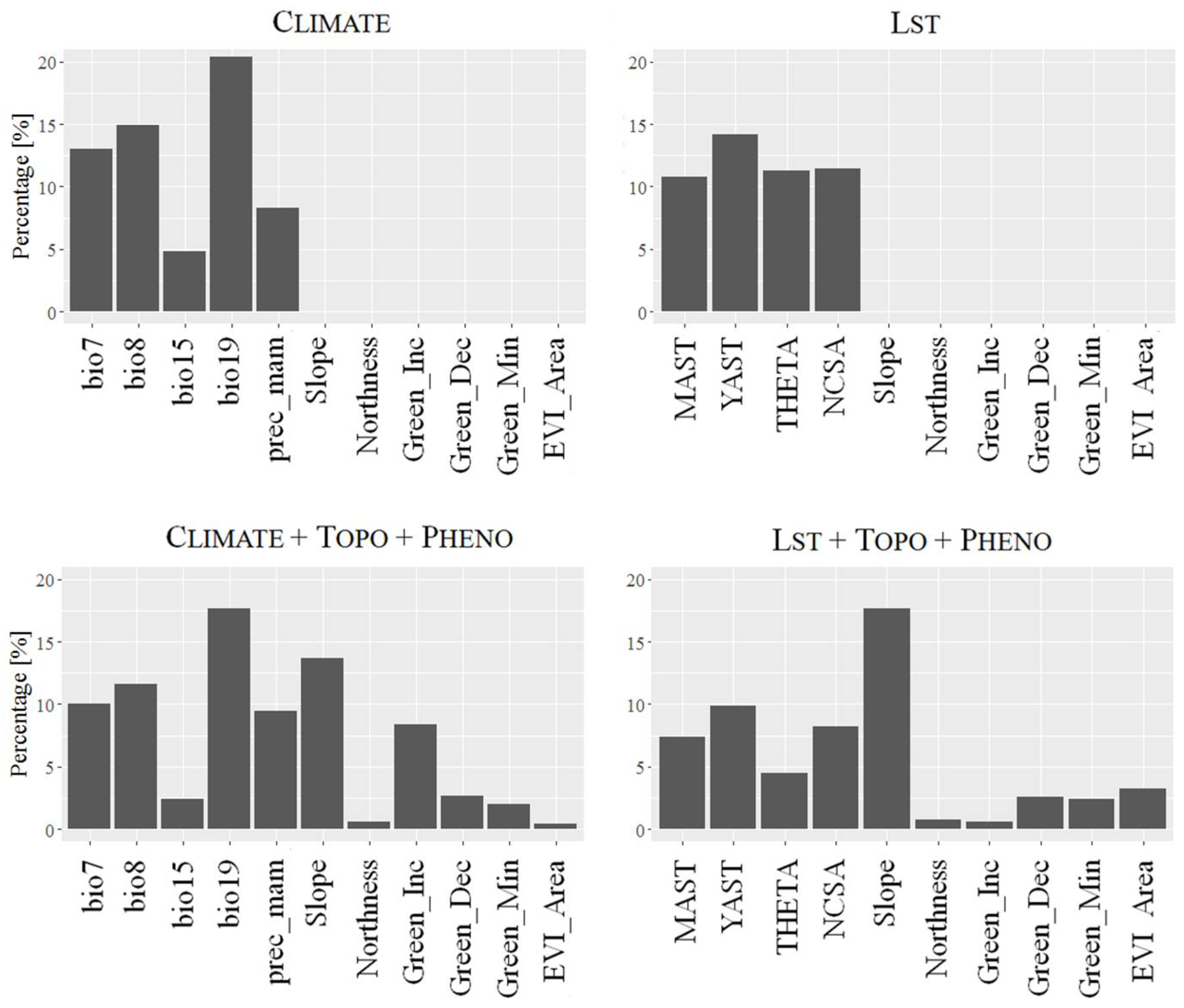
3.2. Variable Importance

We selected 5 climatic variables, 2 topographic variables, 4 land cover metrics, and 4 land surface temperature variables out of 40 potential predictor variables.
In the following, only Climate, Climate + Topo + Pheno, Lst, and Lst + Topo + Pheno will be considered (Figure 3; see Supplementary Material Figure S1 for variable importance of all models). Relative variable importance varied among the four subsets of predictor variables. However, a few general characteristics became evident. Regarding climatic variables (i.e., Climate), Precipitation of Coldest Quarter (bio19) was the most important predictor, followed by Temperature of Wettest Quarter (bio8, i.e., temperature of growing season), Temperature Annual Range (bio7), and Average Precipitation of March, April, and May (prec_mam), whereas Precipitation Seasonality (bio15) had lowest variable importance. Among the topographical variables, the highest importance was found for Slope. Phenological traits derived from Pheno data were always lower in variable importance, whereas temporal metrics, e.g., Onset Greenness Increase (Green_Inc), were superior to the Enhanced Vegetation Index (EVI) metric.
For the Lst model, differences in variable importance were low between all variables, whereas highest variable importance was found for YAST (mean annual temperature). Differences in importance were striking between the predictor variable sets of the Lst + Topo + Pheno model. The highest value of variable importance was found for Slope, followed by YAST (mean annual temperature), NCSA (number of clear-sky acquisitions), MAST (mean annual amplitude of temperature), and THETA (phase shift in days relative to spring equinox on the northern hemisphere), whereas differences in variable importance were rather low between Lst-related variables. For phenological traits, EVI showed highest variable importance.

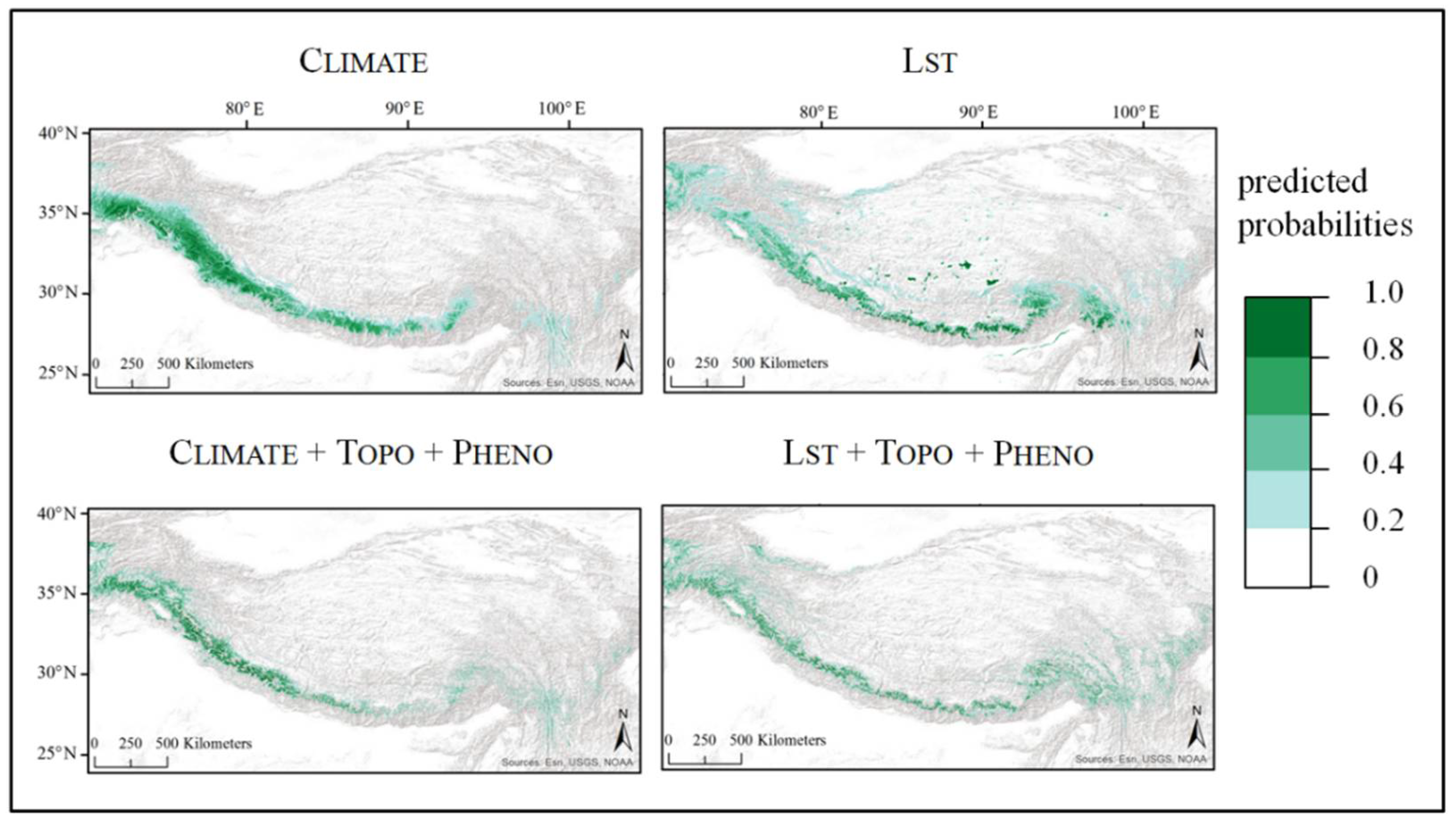
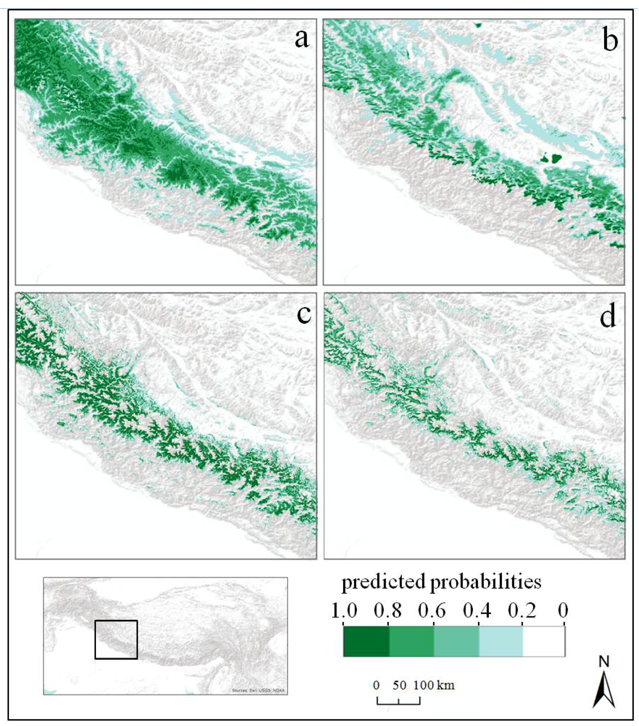
3.3. Ecological Niche Models

The continuous predictions of the models showed noticeable differences (Figure 4). According to the model evaluation measurements, Climate + Topo + Pheno performed best, followed by Lst + Topo + Pheno, whereas Climate was superior to Lst.
It becomes apparent that the core distribution of B. utilis was predicted in the western part of the Himalayan mountain system, whereas only the Lst model predicted a principal distribution in the central part of the mountains. All models showed a uniform distribution along the Himalayan arc. The habitat predicted by Climate tends to be wider in range compared to the other predictions.
Displaying differences in the model predictions in detail (Figure 5), the overall appearance (Figure 4) is better elucidated. The model solely based on climate predictor variables (Climate, Figure 5a) roughly met the lower limit of occurrences compared to the Climate + Topo + Pheno model (Figure 5c), but overpredicted the uppermost limits of B. utilis. Overall, the prediction appears blurry and the broadleaved deciduous treeline could not be distinguished from other vegetation formations (Figure 5a). The Climate + Topo + Pheno model differentiates between slope structures, and clearly delimits the lower distributional range of B. utilis. At higher altitudes, occurrence probability decreases and diminishes (Figure 5c). Comparing Climate + Topo + Pheno models with Lst + Topo + Pheno-based models, similar patterns were observed, whereas the distributional range is predicted more constrained in the latter, leaving a smaller distribution range of B. utilis (Figure 5c,d).
For the model built with remotely sensed temperature-related variables only (Lst, Figure 5b), similar patterns compared to Climate (Figure 5a) could be found. The distribution appears coarse and fuzzy, compared to Climate + Topo + Pheno and Lst + Topo + Pheno models (Figure 5c,d).

4. Discussion

Modelling ecological niches and species distributions in remote high mountain regions like the Himalayas are challenging tasks. Current studies in the field of plant species distribution modelling in the Himalayan mountains mainly use climatic variables to predict species’ distribution or to forecast species range shifts under climate change scenarios (e.g., [7,32,41,70,71,72,73,74,75,76,77]). With regard to Betula utilis, reasonable results were obtained using solely climate for predicting the potential distribution [9,32]. However, the necessity arose for approximating the actual distribution of B. utilis, addressed in this study by evaluating the benefits of incorporating remotely sensed data into the modelling approach.

4.1. Modelling the Ecological Niche of Betula utilis

We found that models combining climate-related variables with remotely sensed topography and phenological traits (Climate + Topo + Pheno and Lst + Topo + Pheno) outperformed models using only one predictor variable set (Climate and Lst). The latter revealed no concise distinction between the vegetation formations (Figure 4 and Figure 5a,b), which indicates the need for further explanatory variables when modelling a species’ realized niche on a large scale, i.e., the entire Himalayan mountain system.
We found that all models predicted suitable habitats for B. utilis as a more or less narrow line stretching along the Himalayan arc, featuring prominently in the western parts. All models predicted lower suitability in the eastern parts of the mountain system, a result which coincides with the occurrence data, and which is in line with the fact that due to the more maritime climate in the east, B. utilis loses its dominance as a treeline species in favour of evergreen Rhododendron species [30]. Model evaluation revealed highest performance for models built on bioclimatic variables combined with remotely sensed topography and phenology data (Climate + Topo + Pheno), emphasizing the improvement achieved by incorporating remotely sensed land cover data for predicting the distribution of B. utilis in the Himalayan mountains. Information on the phenological traits (Greenness Increase, and Greenness Decrease) turned out to be beneficial in refining the ecological niche of B. utilis (e.g., demarcation of other vegetation formations and exposed rocks).
In addition, models built solely on remotely sensed data (Lst + Topo + Pheno) suggested that phenological traits are highly relevant for modelling a more realistic distribution range of the species. The findings indicate that models built on remote sensing data yield promising predictions, which may be of interest in remote areas like the Himalayan mountains due to free availability, global coverage, and fine-scale resolution (<1 km). However, temperature variables alone (Lst) are not fully capable of predicting the distribution range, as they predicted primarily suitable habitats in the central part of the mountain system and some artefacts (i.e., lakes) on the Tibetan plateau. This is to be attributed to the fact that surface temperature is, apart from atmospheric conditions, also affected by land surface characteristics. Moreover, Lst only has a weak proxy for precipitation, namely the number of cloudy/cloud-free days. Consequently, the results using Lst + Topo + Pheno show lower model performance compared to the Climate + Topo + Pheno model, which incorporates precipitation-related and more plant growth specific variables. However, interestingly the Lst model benefits much more from additional predictor sets (i.e., Topo), indicating a certain redundancy between bioclimatic and topographic variables. This is plausible since topographic features are used in the downscaling process of the Chelsa data [33].
Globally, climate governs global patterns of land cover [78], but land cover and climate are not fully independent [13]. Our results confirm topoclimatic variables as the main drivers behind the distribution range, whereas phenological traits substantially contribute to narrow the modelled ecological niche of B. utilis (i.e., more realistic distribution). Similar results were obtained by Parra et al. [79] and Buermann et al. [17] when predicting species distribution across the Amazonian and Andean region. In a hierarchical scheme of environmental controls on species distributions, climatic variables are large-scale determinants, followed by geology, topography, and land cover, which moderate many of the effects of macroclimatic variables [13,16]. Our predictions of the Climate + Topo + Pheno model are consistent with the distribution pattern documented in several vegetation maps showing a narrow band of birch forests forming the upper treeline on north-facing slopes (e.g., [80,81]). However, the actual distribution might be smaller, since topoclimate variables and phenological traits are not the only factors determining habitat suitability. Although not considered in this study, interactions of a whole array of site factors such as ecology of tree species, site history, current biotic interactions, and anthropogenic influences affect treeline species’ spatial distributions [1,30].

4.2. Ecological Interpretation of Predictor Variables

We found two temperature- and three precipitation-related variables (Climate) among the most important for predicting the potential distribution of B. utilis. Mean Temperature of the Wettest Quarter and Temperature Annual Range were most relevant among the temperature-related variables. Growing season air and soil temperatures are considered key factors controlling tree growth at treelines and elevational position of treelines at global scales [1,2]. Much lower growing season temperatures (i.e., Mean Temperature of the Wettest Quarter) and higher average winter temperature (January) in the eastern Himalayas result in lower seasonal temperature variation which favours evergreen Rhododendron species over the deciduous species B. utilis at treelines. In the eastern Himalayas, B. utilis becomes less competitive and evergreen broadleaved species (Rhododendron spp.) are the principal treeline species [30]. By contrast, higher degrees of continentality with higher mean temperatures of warmest months and severe winter coldness lower the competitiveness of Rhododendron spp. at treeline elevations in the western and northwestern Himalayas, and contribute to the higher competitive strength of B. utilis on north-facing slopes.
Precipitation Seasonality, Precipitation of the Coldest Quarter, and Average Precipitation of March, April, and May were the precipitation-related variables, with Precipitation of the Coldest Quarter having the highest variable importance. Precipitation and related factors such as soil moisture and soil nutrient availability can be significant for treeline formation and dynamics [82,83]. Thus, precipitation-related variables potentially limit the climatic space of treeline tree species. The period from November to January was identified as the coldest quarter. Higher winter snowfall in the more continental western parts of the Himalayan region obviously contributes to the competitiveness of B. utilis. Monsoonal summer rains, on the other hand, are of less significance.
Regarding temperature-related remotely sensed variables, all variables proved to be of great importance, but mean annual temperature amplitude (YAST) revealed highest variable importance. Generally, temperature is strongly negatively correlated with altitude (except for cold air inversions in winter months), allowing little room for variation in regional-scale climate data sets [33,84]. This, in turn, leads to similar results for Lst + Topo + Pheno, compared to Climate + Topo + Pheno models, where additional information on phenological traits refined the predicted niche of B. utilis (Figure 4). Interestingly, the number of cloud-free acquisitions NCSA also showed considerable variable importance, indicating that it, despite being a rather poor proxy, contains some information about precipitation.
Furthermore, MAST (mean annual temperature) and THETA (phase shift in days relative to spring equinox) were revealed to be important when modelling the ecological niche of B. utilis. We conclude that THETA, as it represents heat accumulation, shows sensitivity to seasonal snow cover. Vegetation analyses [30,85,86] showed that thickness and duration of snow cover providing sufficient soil moisture at the beginning and at the end of the growing season is one of the principal factors controlling the distribution of B. utilis forests.
The inclusion of topographic variables like Slope led to an improved prediction of climate-only models (both Climate and Lst). This is not surprising, since in topographically highly complex regions like the Himalayas, areas can be predicted as climatically suitable but might be inaccessible due to the slope angle. Betula forests thrive on humid, shady slopes with deeply weathered podzolic soils, and are more or less absent from south-facing slopes, in particular in the more continental W Himalaya [31,32,85].
Due to the steep gradient of hydrothermal conditions in the Himalayas, ranging from subtropical at lower to alpine conditions at higher elevations, diverse vegetation formations are formed, characterized by changing phenological traits. Our results provide compelling evidence that the climate-only models (both Climate and Lst) could be improved with remotely sensed phenological traits. Differences in variable importance were found between Climate + Topo + Pheno and Lst + Topo + Pheno models (Figure 3), the most important phenological traits were Onset Greenness Increase, Onset Greenness Decrease, and the Enhanced Vegetation Index (EVI). Based on these variables, a distinction between evergreen coniferous forests below the birch belt and the evergreen broadleaved krummholz belt and Rhododendron dwarf thickets above could be achieved (Figure 5c,d).
The Climate + Topo + Pheno model revealed the importance of two temporal metrics. The timing of increasing greenness (Onset Greenness Increase) of the B. utilis belt differed significantly from the vegetation formations located below (Kruskal–Wallis Test; p ≤ 0.05). The median green-up date for B. utilis was at 141 Julian days after the snow melt, reflected in the predictor variable Average Precipitation March, April, and May, when sufficient soil moisture for foliation is available. The evergreen coniferous vegetation below had a much earlier green-up date (125 Julian days), whereas the evergreen krummholz belt above had a similar green-up date as the B. utilis belt (141 Julian days). Comparing the averaged dates of vegetation senescence (Decrease of Greenness), no significant differences could be found between the three vegetation formations (Kruskal–Wallis Test; p ≥ 0.05). Nevertheless, the B. utilis belt undergoes senescence earlier (217 Julian days) than the evergreen vegetation formations (after 222 Julian days).
The Lst + Topo + Pheno model showed considerable variable importance of the EVI, which is a convenient measure of plant phenology computed from MODIS surface-reflectance data. The EVI identifies vegetation growth, maturity, and senescence, and thus marks seasonal cycles [51]. The applied EVI identifies the vegetation cycle and records sums of the onset of greenness and of minimum greenness. Hence, at the start of the growing season of evergreens, coniferous vegetation in lower altitudes is earlier, while the growing season ends up later compared to deciduous broadleaved vegetation. This results in the highest median EVI value (37) for vegetation below the treeline, whereas the EVI values for the B. utilis belt (24) and for vegetation formations above the treeline (17) were lower. The amount of light reflected from leaves at visible and infrared wavebands is determined by leaf traits and physiological performance [87]. The information of distinctly different phenological characteristics between the vegetation types was causal to the refinement of the niche models. Furthermore, these seasonal variations can be used to track changes in vegetation phenology [88], whereas shifts in seasonal phenological events are among the first responses at plant and ecosystem levels to climate change [89]. Shifts of flowering to earlier dates have been reported for Rhododendron species [90], and earlier green-up data resulting in an extension of the growing season [91,92] have been reported for the Himalayas. In this context, investigations of underlying climatic factors and quantification of changing plant phenological traits may provide the basis for efficient nature conservation management, expansion of protected areas, and appropriate habitat restoration strategies.

4.3. Application of Remote Sensing Data for Modelling Species’ Distributions

The availability and the quality of input parameters determine model performance. Often, standardized statistically derived parameters do not fully reflect the species’ physiological needs and habitat requirements. Abiotic and biotic data derived from remote sensing may open up new opportunities in analysing and modelling species’ distributions, since they provide response and predictor variables. In an extensive literature review, He et al. [23] and references therein present countless applications of remotely sensed data for modelling species’ distributions. In general, many remote sensing products are adaptable for modelling biota and can be customized in accordance with the study aims.
In the present study, we highlight the benefits of remotely sensed data in deriving tree species occurrences and predictor variables. The potential for future studies lies in the generation of presence and absence data sets, which are highly required in ENM [93]. Due to unique biophysical properties, hyperspectral sensors can detect subtle differences in reflectance based on unique plant chemistries, which is beneficial for identification of plant species [23]. Another advantage is the possibility to incorporate biotic interactions into the models, which are often disregarded due to data limitations [94,95].
Our results emphasize thermal metrics, which could be beneficially incorporated into further treeline studies in remote mountainous regions as they provide freely accessible, complete, and long-term data. Major advantages of Lst-related variables include continuous observations without interpolation and geographical bias and therefore fewer uncertainties [23]. Recent studies showed how Lst data could improve species modelling studies (e.g., [17,96,97]). These parameters offer numerous possibilities, such as tailored predictors in high resolution. As time series data of vegetation characteristics (i.e., phenological metrics) are becoming more and more available, changing habitat suitability can be estimated and incorporated into the model approach. In this way, knowledge can be generated, which is particularly important for modelling spatial expansion of invasive species, extinction risk assessment, and range shifts under future climate change [23].
We conclude that the current state of information may serve as a baseline for future studies, even though the available data derived from remote sensing technology is rather short term. Restrictions in the practical applicability arise from the fact that high resolution satellite imagery is still often very expensive. On the other hand, the free of cost imagery and software is already available and will become more customary in the future. Our results show that, even with freely available data, software model performance could be improved, indicating the potential for future modelling studies.
Airborne technology is a continually expanding field, and high resolution remotely sensed data will provide more insights into spatial patterns and underlying factors in future modelling studies.

5. Conclusions

Modelling ecological niches in remote mountain regions like the Himalayas remains a challenging task due to severe data limitations such as availability of high-quality environmental information. Given the respective climatically and topographically complex terrain, models based on climate variables alone predict the potential distribution of species only, since land cover characteristics are omitted. Nevertheless, climatic gradients determine floristic gradients in high mountain regions, and in turn, phenological traits represent niche proxies. We conclude that the addition of remotely sensed topography and phenological traits as predictor variables leads to improved model performances for the current distribution of B. utilis. It is a conspicuous broadleaved deciduous tree species at the treeline in the Himalayan mountains, allowing a clear separation on the basis of phenological traits from adjacent vegetation types which consist mainly of evergreen coniferous and evergreen deciduous species in the tree layer. It becomes obvious that the inclusion of remotely sensed topography and phenological traits results in a more constrained predicted niche, compared to solely climate based models. Our results underline the relevance of phenological traits to reduce the gap in modelling studies between potential and actual distributions of species over vast, remote, and heterogeneous mountain regions. However, the actual distribution of B. utilis might be smaller than predicted, since topoclimate variables and phenological traits are not the only factors determining habitat suitability, and the resolution of 1 km2 is often too coarse to account for small-scale landscape characteristics such as varying aspects.
We conclude that the approach of substituting bioclimatic variables with annual temperature cycles from remotely sensed Lst data is promising, in particular in regions where sampling efforts are low and sufficient fine-scale climate data are not available.
We further conclude that remotely sensed data make a valuable contribution when modelling the current distribution of B. utilis, since they provide long-term, fine-scale, and freely available observations. Our results emphasize the need for high-resolution data when modelling the actual distribution of treeline species in order to account for the heterogeneous terrain and microclimate. The incorporation of remotely sensed temperature derivates expands the classical approach (i.e., bioclimatic variables and topography) and shows great potential to derive more tailored variables (e.g., temperature of the growing season, precipitation amounts, snow cover) for ecological niche modelling. In future studies, further improvement of ecological niche models could be achieved by incorporating high-resolution remote sensing data.

Supplementary Materials

The following are available online at https://www.mdpi.com/2072-4292/10/6/814/s1. Figure S1: Variable importance for all models based on four predictor variable sets and their combinations. Topography (Topo); Chelsa climate data (Climate); Chelsa climate data and topography (Climate + Topo); Chelsa climate data and Land Cover Dynamics data (Climate + Pheno); Chelsa climate data, topography and Land Cover Dynamics data (Climate + Topo + Pheno); Land Surface Temperature (Lst); Land Surface Temperature and topography (Lst + Topo); Land Surface Temperature and Land Cover Dynamincs data (Lst + Pheno); Land Surface Temperature, topography and Land Cover Dynamics data (Lst + Topo + Pheno); Land Cover Dynamics data (Pheno) and Land Cover Dynamics data and topography (Pheno + Topo) The results for training and test data are displayed (training 80% and testing 20%). Figure S2: Continuous predictions of all models based on four predictor variable sets and their combinations. Topography (Topo); Chelsa climate data (Climate); Chelsa climate data and topography (Climate + Topo); Chelsa climate data and Land Cover Dynamics data (Climate + Pheno); Chelsa climate data, topography and Land Cover Dynamics data (Climate + Topo + Pheno); Land Surface Temperature (Lst); Land Surface Temperature and topography (Lst + Topo); Land Surface Temperature and Land Cover Dynamincs data (Lst + Pheno); Land Surface Temperature, topography and Land Cover Dynamics data (Lst + Topo + Pheno); Land Cover Dynamics data (Pheno) and Land Cover Dynamics data and topography (Pheno + Topo) The results for training and test data are displayed (training 80% and testing 20%). Figure S3: Detailed excerpt of continuous predictions of all models based on four predictor variable sets and their combinations. Topography (Topo); Chelsa climate data (Climate); Chelsa climate data and topography (Climate + Topo); Chelsa climate data and Land Cover Dynamics data (Climate + Pheno); Chelsa climate data, topography and Land Cover Dynamics data (Climate + Topo + Pheno); Land Surface Temperature (Lst); Land Surface Temperature and topography (Lst + Topo); Land Surface Temperature and Land Cover Dynamincs data (Lst + Pheno); Land Surface Temperature, topography and Land Cover Dynamics data (Lst + Topo + Pheno); Land Cover Dynamics data (Pheno) and Land Cover Dynamics data and topography (Pheno + Topo) The results for training and test data are displayed (training 80% and testing 20%).

Author Contributions

M.B. conceived the research project ideas, performed the statistical analyses, wrote the first draft of the manuscript and led the writing. B.B. provided MODIS Land Surface Data. J.O. and B.B. gave statistical advise. J.W. compiled the MODIS Land Cover Data. J.B. and U.S. contributed expert knowledge. All authors critically revised the manuscript.

Funding

This study was carried out in the framework of the TREELINE project and partially funded by the German Research Foundation (DFG, SCHI 436/14-1; BO 1333/4-1) as well as the Cluster of Excellence CliSAP (EXC177) of the University of Hamburg.

Acknowledgments

We would like to express our honest gratitude to Himalayan colleagues, guides and local people who accompanied us on numerous field trips to Betula treelines. Furthermore we would like to thank the three anonymous reviewers for their diligent work and thoughtful suggestions on the earlier version of the manuscript.

Conflicts of Interest

The authors declare no conflict of interest.

References

  1. Holtmeier, F.-K. Mountain Timberlines—Ecology, Patchiness and Dynamics; Advances in Global Change Research; Springer: Berlin/Heidelberg, Germany, 2009; Volume 36. [Google Scholar]
  2. Körner, C. Alpine Treelines—Functional Ecology of the Global High Elevation Tree Limits; Springer: Berlin/Heidelberg, Germany, 2012. [Google Scholar]
  3. Dullinger, S.; Dirnböck, T.; Grabherr, G. Modelling climate-change driven treeline shifts: Relative effects of temperature increase, dispersal and invasibility. J. Ecol. 2004, 92, 241–252. [Google Scholar] [CrossRef]
  4. Thuiller, W.; Lavorel, S.; Araujo, M.B. Niche properties and geographical extent as predictors of species sensitivity to climate change. Glob. Ecol. Biogeogr. 2005, 14, 347–357. [Google Scholar] [CrossRef]
  5. Parolo, G.; Rossi, G.; Ferrarini, A. Toward improved species niche modelling: Arnica montana in the Alps as a case study. J. Appl. Ecol. 2008, 45, 1410–1418. [Google Scholar] [CrossRef]
  6. Thuiller, W. Patterns and uncertainties of species’ range shifts under climate change. Glob. Chang. Biol. 2004, 10, 2020–2027. [Google Scholar] [CrossRef]
  7. Singh, C.P.; Panigrahy, S.; Parihar, J.S.; Dharaiya, N. Modeling environmental niche of Himalayan birch and remote sensing based vicarious validation. Trop. Ecol. 2013, 54, 321–329. [Google Scholar]
  8. Huo, C.; Cheng, G.; Lu, X.; Fan, J. Simulating the effects of climate change on forest dynamics on Gongga Mountain, Southwest China. J. For. Res. Jpn. 2010, 15, 176–185. [Google Scholar] [CrossRef]
  9. Bobrowski, M.; Schickhoff, U. Why input matters: Selection of climate data sets for modelling the potential distribution of a treeline species in the Himalayan region. Ecol. Model. 2017, 359, 92–102. [Google Scholar] [CrossRef]
  10. Tucker, C.J. Red and infrared linear combinations for monitoring vegetation. Remote Sens. Environ. 1979, 8, 127–150. [Google Scholar] [CrossRef]
  11. Strahler, A.H. Stratification of natural vegetation for forest and rangeland inventory using Landsat digital imagery and collateral data. Int. J. Remote Sens. 1981, 2, 15–41. [Google Scholar] [CrossRef]
  12. Hutchinson, C.F. Techniques for combining Landsat and ancillary data for digital classification improvement. Photogramm. Eng. Remote Sens. 1982, 48, 123–130. [Google Scholar]
  13. Thuiller, W.; Araújo, M.B.; Lavorel, S. Do we need land-cover data to model species distributions in Europe? J. Biogeogr. 2004, 31, 353–361. [Google Scholar] [CrossRef]
  14. Luoto, M.; Virkkala, R.; Heikkinen, R.K. The role of land cover in bioclimatic models depends on spatial resolution. Glob. Ecol. Biogeogr. 2007, 16, 34–42. [Google Scholar] [CrossRef]
  15. Zimmermann, N.E.; Edwards, T.C.; Moisen, G.G.; Frescino, T.S.; Blackard, J.A. Remote sensing-based predictors improve distribution models of rare, early successional and broadleaf tree species in Utah. J. Appl. Ecol. 2007, 44, 1057–1067. [Google Scholar] [CrossRef] [PubMed]
  16. Franklin, J. Mapping Species Distributions: Spatial Inference and Prediction; Ecology, Biodiversity and Conservation; Cambridge University Press: Cambridge, UK, 2009. [Google Scholar]
  17. Buermann, W.; Saatchi, S.; Smith, T.B.; Zutta, B.R.; Chaves, J.A.; Milá, B.; Graham, C.H. Predicting species distributions across the Amazonian and Andean regions using remote sensing data. J. Biogeogr. 2008, 35, 1160–1176. [Google Scholar] [CrossRef]
  18. Feilhauer, H.; He, K.S.; Rocchini, D. Modeling Species Distribution Using Niche-Based Proxies Derived from Composite Bioclimatic Variables and MODIS NDVI. Remote Sens. 2012, 4, 2057–2075. [Google Scholar] [CrossRef]
  19. Braunisch, V.; Patthey, P.; Arlettaz, R. Where to Combat Shrub Encroachment in Alpine Timberline Ecosystems. Combining Remotely-Sensed Vegetation Information with Species Habitat Modelling. PLoS ONE 2016, 11, e0164318. [Google Scholar] [CrossRef] [PubMed]
  20. West, A.M.; Evangelista, P.H.; Jarnevich, C.S.; Young, N.E.; Stohlgren, T.J.; Talbert, C.; Talbert, M.; Morisette, J.; Anderson, R. Integrating Remote Sensing with Species Distribution Models, Mapping Tamarisk Invasions Using the Software for Assisted Habitat Modeling (SAHM). J. Vis. Exp. 2016, 116. [Google Scholar] [CrossRef] [PubMed]
  21. Peterson, A.T.; Nakazawa, Y. Environmental data sets matter in ecological niche modelling: An example with Solenopsis invicta and Solenopsis richteri. Glob. Ecol. Biogeogr. 2007, 17, 135–144. [Google Scholar] [CrossRef]
  22. Cord, A.F.; Klein, D.; Mora, F.; Dech, S. Comparing the suitability of classified land cover data and remote sensing variables for modeling distribution patterns of plants. Ecol. Model. 2014, 272, 129–140. [Google Scholar] [CrossRef]
  23. He, K.S.; Bradley, B.A.; Cord, A.F.; Rocchini, D.; Tuanmu, M.-N.; Schmidtlein, S.; Turner, W.; Wegmann, M.; Pettorelli, N. Will remote sensing shape the next generation of species distribution models? Remote Sens. Ecol. Conserv. 2015, 1, 4–18. [Google Scholar] [CrossRef]
  24. Franklin, J. Predictive vegetation mapping—Geographic modelling of biospatial patterns in relation to environmental gradients. Prog. Phys. Geogr. 1995, 19, 474–499. [Google Scholar] [CrossRef]
  25. Forrest, J.; Miller-Rushing, A.J. Toward a synthetic understanding of the role of phenology in ecology and evolution. Philos. Trans. R. Soc. Lond. B Biol. Sci. 2010, 365, 3101–3112. [Google Scholar] [CrossRef] [PubMed]
  26. Polgar, C.A.; Primack, R.B. Leaf-out phenology of temperate woody plants: From trees to ecosystems. New Phytol. 2011, 191, 926–941. [Google Scholar] [CrossRef] [PubMed]
  27. Morisette, J.T.; Richardson, A.D.; Knapp, A.K.; Fisher, J.I.; Graham, E.A.; Abatzoglou, J.; Wilson, B.E.; Breshears, D.D.; Henebry, G.M.; Hanes, J.M.; et al. Tracking the rhythm of the seasons in the face of global change: Phenological research in the 21st century. Front. Ecol. Environ. 2009, 7, 253–260. [Google Scholar] [CrossRef]
  28. Wilfong, B.N.; Gorchov, D.L.; Henry, M.C. Detecting an invasive shrub in deciduous forest understories using remote sensing. Weed Sci. 2009, 57, 512–520. [Google Scholar] [CrossRef]
  29. Tuanmu, M.-N.; Viña, A.; Bearer, S.; Xu, W.; Ouyang, Z.; Zhang, H.; Liu, J. Mapping understory vegetation using phenological characteristics derived from remotely sensed data. Remote Sens. Environ. 2010, 114, 1833–1844. [Google Scholar] [CrossRef]
  30. Schickhoff, U. The upper timberline in the Himalaya, Hindu Kush and Karakorum: A review of geographical and ecological aspects. In Mountain Ecosystems. Studies in Treeline Ecology; Broll, G.B., Keplin, B., Eds.; Springer: Berlin/Heidelberg, Germany, 2005; pp. 275–354. [Google Scholar]
  31. Miehe, G. Landscapes of Nepal. In Nepal: An Introduction to the Natural History, Ecology and Human Environment of the Himalayas; Miehe, G., Pendry, C.A., Chaudhary, R.P., Eds.; Royal Botanic Garden Edinburgh: Edinburgh, UK, 2015; pp. 7–16. [Google Scholar]
  32. Bobrowski, M.; Gerlitz, L.; Schickhoff, U. Modelling the potential distribution of Betula utilis in the Himalaya. Glob. Ecol. Conserv. 2017, 11, 69–83. [Google Scholar] [CrossRef]
  33. Karger, D.N.; Conrad, O.; Böhner, J.; Kawohl, T.; Kreft, H.; Soria-Auza, R.W.; Zimmermann, N.; Linder, H.P.; Kessler, M. Climatologies at high resolution for the earth land surface areas. arXiv, 2016; arXiv:1607.00217. [Google Scholar]
  34. USGS. Shuttle Radar Topography Mission, 1 Arc Second Scene SRTM_u03_n008e004, Unfilled Unfinished 2.0; Global Land Cover Facility, University of Maryland: College Park, MD, USA, 2004.
  35. LP DAAC. NASA Land Processes Distributed Active Archive Center, USGS/Earth Resources Observation and Science (EROS) Center, 2012. Available online: https://lpdaac.usgs.gov/data_access/data_pool (accessed on 14 June 2017).
  36. Bechtel, B. A new global climatology of annual land surface temperature. Remote Sens. 2015, 7, 2850–2870. [Google Scholar] [CrossRef]
  37. Troll, C. The three-dimensional zonation of the Himalayan system. In Geoecology of the High-Mountain Regions of Eurasia; Troll, C., Ed.; Erdwissenschaftliche Forschung, Franz Steiner Verlag: Wiesbaden, Germany, 1972; Volume 4, pp. 264–275. [Google Scholar]
  38. Miehe, G.; Miehe, S.; Böhner, J.; Bäumler, R.; Ghimire, S.K.; Bhattarai, K.; Chaudhary, R.P.; Subedi, M.; Jha, P.K.; Pendry, C. Vegetation ecology. In Nepal: An Introduction to the Natural History, Ecology and Human Environment of the Himalayas; Miehe, G., Pendry, C.A., Chaudhary, R.P., Eds.; Royal Botanic Garden Edinburgh: Edinburgh, UK, 2015; pp. 385–472. [Google Scholar]
  39. Zurick, D.; Pacheco, J. Illustrated Atlas of the Himalaya; The University Press of Kentucky: Lexington, KY, USA, 2006. [Google Scholar]
  40. Polunin, O.; Stainton, A. Flowers of the Himalaya; Oxford University Press: New Delhi, India, 1984. [Google Scholar]
  41. Schickhoff, U.; Bobrowski, M.; Jürgen Böhner, J.; Bürzle, B.; Chaudari, R.P.; Gerlitz, L.; Heyken, H.; Lange, J.; Müller, M.; Scholten, T.; et al. Do Himalayan treelines respond to recent climate change? An evaluation of sensitivity indicators. Earth Syst. Dyn. 2015, 6, 245–265. [Google Scholar] [CrossRef]
  42. GBIF.org: Biodiversity Occurrence Data provided by: Missouri Botanical Garden, Royal Botanic Garden Edinburgh and The Himalayan Uplands Plant Database, Accessed through GBIF Data Portal. Available online: http://www.gbif.org (accessed on 10 January 2016).
  43. Google Earth; ver. 7.1.1.1888; Google LLC (“Google”): Mountain View, CA, USA, 2015.
  44. Paulsen, J.; Körner, C. A climate-based model to predict potential treeline position around the globe. Alp. Bot. 2014, 124, 1–12. [Google Scholar] [CrossRef]
  45. Irl, S.D.H.; Anthelme, F.; Harter, D.E.V.; Jentsch, A.; Lotter, E.; Steinbauer, M.J.; Beierkuhnlein, C. Patterns of island treeline elevation—A global perspective. Ecography 2015, 38, 1–10. [Google Scholar] [CrossRef]
  46. Dormann, C.F.; Elith, J.; Bacher, S.; Buchmann, C.; Carl, G.; Carré, G.; Marquéz, J.R.; Gruber, B.; Lafourcade, B.; Leitão, P.J.; et al. Collinearity: A review of methods to deal with it and a simulation study evaluating their performance. Ecography 2013, 36, 27–46. [Google Scholar] [CrossRef]
  47. Hijmans, R.J.; Cameron, S.E.; Parra, J.L.; Jones, P.G.; Jarvis, A. Very high resolution interpolated climate surfaces for global land areas. Int. J. Climatol. 2005, 25, 1965–1978. [Google Scholar] [CrossRef]
  48. Liang, E.; Dawadi, B.; Pederson, N.; Eckstein, D. Is the growth of birch at the upper timberline in the Himalayas limited by moisture or by temperature? Ecology 2014, 95, 2453–2465. [Google Scholar] [CrossRef]
  49. Schickhoff, U.; Bobrowski, M.; Böhner, J.; Bürzle, B.; Chaudhary, R.P.; Gerlitz, L.; Lange, J.; Müller, M.; Scholten, T.; Schwab, N. Climate change and treeline dynamics in the Himalaya. In Climate Change, Glacier Response, and Vegetation Dynamics in the Himalaya; Singh, R.B., Schickhoff, U., Mal, S., Eds.; Springer: Cham, Switzerland, 2016; pp. 271–306. [Google Scholar]
  50. Conrad, O.; Bechtel, B.; Bock, M.; Dietrich, H.; Fischer, E.; Gerlitz, L.; Wehberg, J.; Wichmann, V.; Böhner, J. System for Automated Geoscientific Analyses (SAGA) v. 2.1.4. Geosci. Model Dev. 2015, 8, 1991–2007. [Google Scholar] [CrossRef]
  51. Huete, A.; Didan, K.; Miura, T.; Rodriguez, E.P.; Gao, X.; Ferreira, L.G. Overview of the radiometric and biophysical performance of the MODIS vegetation indices. Remote Sens. Environ. 2002, 83, 195–213. [Google Scholar] [CrossRef]
  52. Zhang, X.; Friedl, M.A.; Schaaf, C.B.; Strahler, A.H.; Hodges, J.C.F.; Gao, F.; Reed, B.C.; Huete, A. Monitoring vegetation phenology using MODIS. Remote Sens. Environ. 2003, 84, 471–475. [Google Scholar] [CrossRef]
  53. Zhang, X.; Friedl, M.A.; Schaaf, C.B. Global vegetation phenology from Moderate Resolution Imaging Spectroradiometer (MODIS): Evaluation of global patterns and comparison with in situ measurements. J. Geophys. Res. 2006, 111. [Google Scholar] [CrossRef]
  54. Ganguly, D.; Rasch, P.J.; Wang, H.; Yoon, J.-H. Climate response of the South Asian monsoon system to anthropogenic aerosols. J. Geophys. Res. 2012, 117. [Google Scholar] [CrossRef]
  55. Wan, Z. New refinements and validation of the MODIS Land-Surface Temperature/Emissivity products. Remote Sens. Environ. 2008, 112, 59–74. [Google Scholar] [CrossRef]
  56. Bechtel, B. Robustness of annual cycle parameters to characterize the urban thermal landscapes. IEEE Geosci. Remote Sens. Lett. 2012, 9, 876–880. [Google Scholar] [CrossRef]
  57. Bechtel, B.; Sismanidis, P. Time series analysis of moderate resolution land surface temperatures. In Remote Sensing: Time Series Image Processing; Weng, Q., Ed.; Taylor & Francis: Abingdon, UK, 2017. [Google Scholar]
  58. McCullagh, P.; Nelder, J.A. Generalized Linear Models; Chapman and Hall: London, UK, 1989. [Google Scholar]
  59. Nelder, J.A.; Wedderburn, R.W.M. Generalized linear models. J. R. Stat. Soc. A 1972, 135. [Google Scholar] [CrossRef]
  60. Austin, M.P. A silent clash of paradigms: Some inconsistencies in community ecology. Oikos 1999, 86, 170–178. [Google Scholar] [CrossRef]
  61. Akaike, H. A new look at the statistical model identification. IEEE Trans. Autom. Control 1974, 19, 716–723. [Google Scholar] [CrossRef]
  62. Burnham, K.P.; Anderson, D.R. Model Selection and Multimodel Inference: A Practical Information-Theoretic Approach, 2nd ed.; Springer: New York, NY, USA, 2002. [Google Scholar]
  63. Guisan, A.; Edwards, T.C., Jr.; Hastie, T. Generalized linear and generalized additive models in studies of species distributions: Setting the scene. Ecol. Model. 2002, 157, 89–100. [Google Scholar] [CrossRef]
  64. VanderWal, J.; Shoo, L.P.; Graham, C.C.; William, S.E. Selecting pseudo-absence data for presence-only distribution modeling: How far should you stray from what you know? Ecol. Model. 2009, 220. [Google Scholar] [CrossRef]
  65. Barbet-Massin, M.; Jiguet, F.; Albert, C.H.; Thuiller, W. Selecting pseudo-absences for species distribution models: How, where and how many? Methods Ecol. Evol. 2012, 3, 327–338. [Google Scholar] [CrossRef]
  66. Kuhn, M.; Johnson, K. Applied Predictive Modeling; Springer: New York, NY, USA, 2013. [Google Scholar]
  67. Nagelkerke, N. A note on a general definition of the coefficient ofdetermination. Biometrika 1991, 78, 691–692. [Google Scholar] [CrossRef]
  68. R Core Team, version: 3.1.3, 2015, R: A Language and Environment for Statistical Computing. R Foundation for Statistical Computing, Vienna, Austria. Available online: http://www.R-project.org/ (accessed on 1 May 2015).
  69. ESRI. ArcGIS Desktop: Release 10.1.; Environmental Systems Research Institute: Redlands, CA, USA, 2012. [Google Scholar]
  70. Menon, S.; Choudhury, B.I.; Khan, M.L.; Peterson, A.T. Ecological niche modelling and local knowledge predict new populations of Gymnocladus assamicus, a critically endangered tree species. Endanger. Species Res. 2010, 11, 175–181. [Google Scholar] [CrossRef]
  71. Menon, S.; Khan, M.L.; Paul, A.; Peterson, A.T. Rhododendron species in the Indian eastern Himalayas: New approaches to understanding rare plant species distributions. JARS 2012, 38, 78–84. [Google Scholar]
  72. Kumar, P. Assessment of impact of climate change on Rhododendrons in Sikkim Himalayas using Maxent modelling: Limitations and challenges. Biodivers. Conserv. 2012, 21, 1251–1266. [Google Scholar] [CrossRef]
  73. Jaryan, V.; Datta, A.; Uniyal, S.K.; Kumar, A.; Gupta, R.C.; Singh, R.D. Modelling potential distribution of Sapium sebiferum—An invasive tree species in western Himalaya. Curr. Sci. 2013, 105, 1282–1288. [Google Scholar]
  74. Gajurel, J.P.; Werth, S.; Shrestha, K.K.; Scheidegger, C. Species distribution modeling of Taxus wallichiana (Himalayan Yew) in Nepal Himalaya. Asian J. Conserv. Biol. 2014, 3, 127–134. [Google Scholar]
  75. Ranjitkar, S.; Kindt, R.; Sujakhu, N.M.; Hart, R.; Guo, W.; Yang, X.; Shrestha, K.K.; Xu, J.; Luedeling, E. Separation of the bioclimatic spaces of Himalayan tree rhododendron species predicted by ensemble suitability models. Glob. Ecol. Conserv. 2014, 1, 2–12. [Google Scholar] [CrossRef]
  76. Shrestha, U.B.; Bawa, K.S. Impact of climate change on potential distribution of Chinese Caterpillar Fungus (Ophiocordyceps chinensis) in Nepal Himalaya. PLoS ONE 2014, 9, e106405. [Google Scholar] [CrossRef] [PubMed]
  77. Manish, K.; Telwala, Y.; Nautiyal, D.C.; Pandit, M.K. Modelling the impacts of future climate change on plant communities in the Himalaya: A case study from eastern Himalaya, India. MESE 2016, 2, 1–12. [Google Scholar] [CrossRef]
  78. Dale, V.H. The relationship between land-use change and climate change. Ecol. Appl. 1997, 7, 753–769. [Google Scholar] [CrossRef]
  79. Parra, J.L.; Graham, C.C.; Freile, J.F. Evaluating alternative data sets for ecological niche models of birds in the Andes. Ecography 2004, 27, 350–360. [Google Scholar] [CrossRef]
  80. Schweinfurth, U. Die horizontale und vertikale Verbreitung der Vegetation im Himalaya. In Bonner Geographische Abhandlungen 20; Dümmlers: Bonn, Germany, 1957. [Google Scholar]
  81. Schickhoff, U. Die Verbreitung der Vegetation im Kaghan-Tal (Westhimalaya, Pakistan) und ihre kartographische Darstellung im Maßstab 1:150.000. Erdkunde 1994, 48, 92–110. [Google Scholar] [CrossRef]
  82. Müller, M.; Schwab, N.; Schickhoff, U.; Böhner, J.; Scholten, T. Soil temperature and soil moisture patterns in a Himalayan alpine treeline ecotone. Arct. Antarct. Alp. Res. 2016, 48, 501–521. [Google Scholar] [CrossRef]
  83. Müller, M.; Schickhoff, U.; Scholten, T.; Drollinger, S.; Böhner, J.; Chaudhary, R.P. How do soil properties affect alpine treelines? General principles in a global perspective and novel findings from Rolwaling Himal, Nepal. Prog. Phys. Geogr. 2016, 40, 135–160. [Google Scholar] [CrossRef]
  84. Soria-Auza, R.; Kessler, M.; Bach, K.; Barajas-Barbosa, P.; Lehnert, M.; Herzog, S.; Böhner, J. Impact of the quality of climate models for modelling species occurrences in countries with poor climatic documentation: A case study from Bolivia. Ecol. Model. 2010, 221, 1221–1229. [Google Scholar] [CrossRef]
  85. Schickhoff, U. Himalayan forest-cover changes in historical perspective. A case study in the Kaghan Valley, Northern Pakistan. Mt. Res. Dev. 1995, 15, 3–18. [Google Scholar] [CrossRef]
  86. Schickhoff, U. The impact of the Asian summer monsoon on forest distribution patterns, ecology and regeneration north of the main Himalayan range (E Hindukush, Karakorum). Phytocoenologia 2000, 30, 633–654. [Google Scholar] [CrossRef]
  87. Price, J. How unique are spectral signatures? Remote Sens. Environ. 1994, 49, 181–186. [Google Scholar] [CrossRef]
  88. Beck, P.S.A.; Jönsson, P.; Høgda, K.-A.; Karlsen, S.R.; Eklundh, L.; Skidmore, A.K. A ground-validated NDVI dataset for monitoring vegetation dynamics and mapping phenology in Fennoscandia and the Kola Peninsula. Int. J. Remote Sens. 2007, 28, 4311–4330. [Google Scholar] [CrossRef]
  89. Badeck, F.-W.; Bondeau, A.; Böttcher, K.; Doktor, D.; Lucht, W.; Schaber, J.; Sitch, S. Responses of spring phenology to climate change. New Phytol. 2004, 162, 295–309. [Google Scholar] [CrossRef]
  90. Xu, J.; Grumbine, R.E.; Shrestha, A.; Eriksson, M.; Yang, X.; Wang, Y.; Wilkes, A. Melting Himalayas: Cascading effects of climate change on water, biodiversity, and livelihoods. Conserv. Biol. 2009, 23, 520–530. [Google Scholar] [CrossRef] [PubMed]
  91. Panday, P.K.; Ghimire, B. Time-series analysis of NDVI from AVHRR data over the Hindu Kush–Himalayan region for the period 1982–2006. Int. J. Remote Sens. 2012, 33, 6710–6721. [Google Scholar] [CrossRef]
  92. Shrestha, U.B.; Gautam, S.; Bawa, K.S. Widespread Climate Change in the Himalayas and Associated Changes in Local Ecosystems. PLoS ONE 2012, 7, e36741. [Google Scholar] [CrossRef] [PubMed] [Green Version]
  93. Fithian, W.; Elith, J.; Hastie, T.; Keith, D.A. Bias correction in species distribution models: Pooling survey and collection data for multiple species. Methods Ecol. Evol. 2015, 6, 424–438. [Google Scholar] [CrossRef] [PubMed]
  94. Kissling, W.D.; Dormann, C.F.; Groeneveld, J.; Hickler, T.; Kühn, I.; McInerny, G.J.; Montoya, J.M.; Römermann, C.; Schiffers, K.; Schurr, F.M.; et al. Towards novel approaches to modelling biotic interactions in multispecies assemblages at large spatial extents. J. Biogeogr. 2012, 39, 2163–2178. [Google Scholar] [CrossRef]
  95. Dormann, C.F.; Bobrowski, M.; Dehling, M.; Harris, D.J.; Hartig, F.; Lischke, H.; Moretti, M.D.; Pagel, J.; Pinkert, S.; Schleuning, M.; et al. Biotic interactions in species distribution modelling: Ten questions to guide interpretation and avoid false conclusions. Glob. Ecol. Biogeogr. 2018. [Google Scholar] [CrossRef]
  96. Bisrat, S.A.; White, M.A.; Beard, K.H.; Richard Cutler, D. Predicting the distribution potential of an invasive frog using remotely sensed data in Hawaii. Divers. Distrib. 2012, 18, 648–660. [Google Scholar] [CrossRef]
  97. Still, C.J.; Pau, S.; Edwards, E.J. Land surface skin temperature captures thermal environments of C3 and C4 grasses. Glob. Ecol. Biogeogr. 2014, 23, 286–296. [Google Scholar] [CrossRef]
Figure 1. Occurrences of Betula utilis along the Himalayan arc (N = 1041).
Remotesensing 10 00814 g001
Figure 2. Overview of the predictor sets used in the modelling procedure for estimating the ecological niche of Betula utilis.
Remotesensing 10 00814 g002
Figure 3. Variable importance of the models using four different predictor variable sets: Chelsa climate data and Land Cover Dynamics data (Climate + Pheno); Chelsa climate data (Climate); Land Surface Temperature and Land Cover Dynamics data (Lst + Pheno); Land Cover Dynamics data (Pheno) and Land Surface Temperature (Lst) For variable description, see Table 1 and for variable importance of all models Supplementary Material Figure S1.
Remotesensing 10 00814 g003
Figure 4. Continuous predictions of the models using four different predictor variable sets: Chelsa climate data (Climate); Land Surface Temperature (Lst); and both combined with Topography (Topo) and Land Cover Dynamics data (Pheno). For continuous prediction of all models, see Supplementary Material Figure S2.
Remotesensing 10 00814 g004
Figure 5. Detailed excerpt of continuous predicted occurrence probability using four different predictor variable sets: (a) Chelsa climate data (Climate); (b) Land Surface Temperature (Lst); (c) Chelsa climate data, Topography and Land Cover Dynamics data (Climate + Topo + Pheno); (d) Land Surface Temperature, Topography and Land Cover Dynamics data (Lst + Topo + Pheno). For detailed continuous prediction of all models, see Supplementary Material Figure S3.
Remotesensing 10 00814 g005
Table 1. Predictor sets with variables used for modelling the ecological niche of Betula utilis.
Input SetLabel VariableScaling FactorUnitsUsed for Modelling
Climatebio1Annual Mean Temperature1Degree Celsius
Chelsabio2Mean Diurnal Range (Mean of monthly (max temp–min temp))1Degree Celsius
bio3Isothermality (bio2/bio7)1Dimensionless
bio4Temperature Seasonality (Stand. Dev.)100Degree Celsius
bio5Max Temperature of Warmest Month1Degree Celsius
bio6Min Temperature of Coldest Month1Degree Celsius
bio7Temperature Annual Range (bio5–bio6)1Degree CelsiusX
bio8Mean Temperature of Wettest Quarter1Degree CelsiusX
bio9Mean Temperature of Driest Quarter1Degree Celsius
bio10Mean Temperature of Warmest Quarter1Degree Celsius
bio11Mean Temperature of Coldest Quarter1Degree Celsius
bio12Annual Precipitation1Millimetre
bio13Precipitation of Wettest Month1Millimetre
bio14Precipitation of Driest Month1Millimetre
bio15Precipitation Seasonality (Coefficient of Variation)100PercentageX
bio16Precipitation of Wettest Quarter1Millimetre
bio17Precipitation of Driest Quarter1Millimetre
bio18Precipitation of Warmest Quarter1Millimetre
bio19Precipitation of Coldest Quarter1MillimetreX
prec_mayAverage Precipitation May1Millimetre
prec_mamAverage Precipitation March, April, May1MillimetreX
TopoAltAltitude1Meters
TopographyNorthnessNorthness1RadiansX
EastnessEastness1Radians
SlopeSlope angle1PercentageX
PhenoGreen_IncOnset Greenness Increase1DaysX
MODIS Land Green_MaxOnset Greenness Maximum1DaysX
Cover DynamicsGreen_DecOnset Greenness Decrease1DaysX
Green_MinOnset Greenness Minimum1Days
EVI_MinNBAR EVI Onset Greenness Min0.0001EVI value
EVI_MaxNBAR EVI Onset Greenness Max0.0001EVI value
EVI_AreaNBAR EVI Area0.01EVI areaX
Dym_QCDynamics QC1Concatenated flags
LstMASTMean annual land surface temperature1KX
MODIS Land YASTMean annual amplitude of land surface temperature1KX
Surface TemperatureTHETAPhase shift relative to spring equinox on the Northern hemisphere1daysX
RMSEInter-diurnal and inter-annual variability (Root Mean Squared Error of fit)1KX
NCSANumber of clear-sky aquisitions1--X
MaxDaytime mean maximum annual surface temperature1K
MinDaytime mean minimum annual surface temperature1K
Table 2. Model evaluation results with regard to several performance measures for five averaged generalized linear model runs based on the four predictor variable sets and their combinations: Topography (Topo); Chelsa climate data (Climate); Land Cover Dynamics data (Pheno); Land Surface Temperature (Lst). The results for training and test data are displayed (training 80% and testing 20%, means of 5 runs).
ModelAkaike Information CriterionArea under the CurveCohen’s KappaPseudo R2 Explained VarianceRMSE
TestTestTestTrainTestTrainTest
Topo7780.920.410.480.480.260.26
Climate6880.930.590.580.560.230.24
Climate + Topo5770.960.660.650.650.210.21
Climate + Pheno6250.940.660.640.630.210.22
Climate + Topo + Pheno5350.960.720.700.690.190.19
Lst8680.910.310.410.410.260.27
Lst + Topo6420.950.600.590.600.230.22
Lst + Pheno7550.920.540.510.640.240.23
Lst + Topo + Pheno5940.960.660.640.650.210.21
Pheno11480.770.010.180.150.300.31
Pheno + Topo7220.930.510.550.540.240.24

