Abstract
The Upper Zambezi River Basin (UZRB) delineates a complex region of topographic, soil and rainfall gradients between the Congo rainforest and the Kalahari Desert. Satellite imagery shows permanent wetlands in low-lying convergence zones where surface–groundwater interactions are vigorous. A dynamic wetland classification based on MODIS Nadir BRDF-Adjusted Reflectance is developed to capture the inter-annual and seasonal changes in areal extent due to groundwater redistribution and rainfall variability. Simulations of the coupled water–carbon cycles of seasonal wetlands show nearly double rates of carbon uptake as compared to dry areas, at increasingly lower water-use efficiencies as the dry season progresses. Thus, wetland extent and persistence into the dry season is key to the UZRB’s carbon sink and water budget. Whereas groundwater recharge governs the expansion of wetlands in the rainy season under large-scale forcing, wetland persistence in April–June (wet–dry transition months) is tied to daily morning fog and clouds, and by afternoon land–atmosphere interactions (isolated convection). Rainfall suppression in July–September results from colder temperatures, weaker regional circulations, and reduced instability in the lower troposphere, shutting off moisture recycling in the dry season despite high evapotranspiration rates. The co-organization of precipitation and wetlands reflects land–atmosphere interactions that determine wetland seasonal persistence, and the coupled water and carbon cycles.
1. Introduction
Wetlands make up less than 9% of global land area, yet they are the largest terrestrial biological source of carbon and the largest source of methane emissions worldwide [1]. Acting as storm buffers and sites of groundwater recharge, wetlands are sensitive to environmental changes, particularly in response to precipitation events and temperature fluctuations [2]. Changes in rainfall or groundwater contributions can alter the areal extent, persistence, and integrity of wetlands and subsequently result in the loss of important wetland functions, such as the capacity to store and filter water, as well as the ability to balance carbon storage and greenhouse gas emissions [1,3,4,5]. As such, describing the changes of wetland areal extent in response to meteorological conditions and subsurface discharge is important for understanding the coupled water–carbon cycles, and land–atmosphere interactions, among other areas of research [6].
Globally, wetland inventories lack the information necessary to locate and maintain wetland areas, and wetland loss is documented poorly since few countries have accurate maps of wetland areas for the past century or so (e.g., [7]). Roughly half of the world’s wetland areas have been lost due to human activities, and many existing wetlands are degraded from drainage, agriculture, and dam construction, among other uses [1,8]. Therefore, it is increasingly important to accurately map wetlands dynamically, particularly in order to target wetland restoration and conservation efforts. The Upper Zambezi River Basin (UZRB) in Sub-Saharan Africa is an area of complex topography and hydrometeorology where interactions between the Angola High Plateau (AHP), the Inter-tropical Convergence Zone (ITCZ), and the Congo Air Boundary Zone (CABZ) determine the spatial and temporal distribution of water resources, and inter-annual climate variability likely maps to the variability observed in vegetation and wetland density [9]. However, long-term records and detailed spatial observations of surface water, groundwater, and boundary layer water, carbon and energy fluxes are scarce for this region.
In order to accurately describe spatiotemporal changes in ecosystem water availability, surface–groundwater interactions must be considered at the floodplain scale. Characterization of surface–groundwater interactions in the UZRB requires dynamic identification of ephemeral wetland areas that expand to store water during the wet season, and recede with aquifer discharge in the dry season. Methods for determining the spatial and temporal variation of wetlands using remote sensing observations include: delineating wetland extent with active [10,11,12,13,14,15,16,17] and passive microwave sensors [18,19]; classifying wetland areas with optical imagers including Landsat ETM+, SPOT, ASTER, and MODIS [20,21,22,23,24,25,26,27]; and inferring wetland area from indices derived from infrared satellite bands sensitive to water, for example, the Normalized Difference Water Index (NDWI) [28,29]. The spectral wavebands of microwave sensors and optical imagers tend to miss smaller scale features when used to delineate wetlands and have difficulty distinguishing narrow wetlands, canopy density, and the spectral signatures of other land cover classes [24,30,31]. Indices constructed from visible and infrared satellite reflectance bands highlight specific surface properties like greenness and water content [28,29,31]. While these indices are unable to distinguish effectively between different wetland types or vegetation species, they map the physical surface characteristics that are indicative of wetlands. We propose a combined approach where four different indices constructed from the visible and infrared surface reflectances are treated as predictors for wetlands within a logistic regression model that allows for dynamic wetland mapping.
Understanding the role of the wetland vegetation in the water budget of the UZRB is crucial for evaluating the impact of changes in wetland extent on land–atmosphere interactions. It is of particular importance to evaluate how seasonal precipitation impacts the persistence of wetlands through the dry season and, in turn, how persistent wetlands support environments favorable to rainfall processes. These areas serve as an additional moisture source for vegetation undergoing photosynthesis and evapotranspiration. Thus, inter-annual and inter-seasonal variability in wetland extent have implications for both the carbon and water cycles. This manuscript aims to show how changes in wetland extent relates to local precipitation patterns and how ephemeral wetland persistence impacts the coupled water–carbon cycles.
2. Data and Methods
2.1. Study Area
The UZRB serves as the headwater catchment of the fourth largest river in Africa, provides essential freshwater resources to arid and semi-arid regions within its boundaries, and recharges the Northern Kalahari Aquifer (Figure 1). This aquifer directly underlies this region and impacts vegetation growth in the floodplains via nonlinear interactions between surface water and groundwater [32]. MODIS Normalized Difference Vegetation Index (NDVI) data show the inter-annual variability in breaks in vegetation (Figure 2). Shallow (~3 m active depth) and clayey soils in the UZRB give way to seasonal waterlogging, especially along drainage lines, favoring the establishment of wetlands [32]. Woodland savanna, grasslands and miombo dominate the UZRB’s diverse ecosystem, marking a complex transition zone between the Congo tropical rainforest and the Kalahari Desert that reflects spatial rainfall gradients.
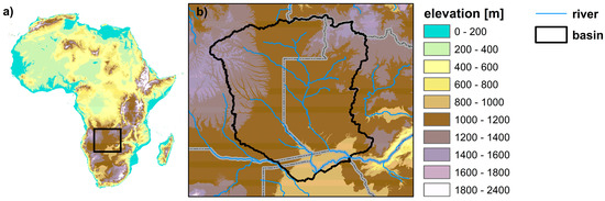
Figure 1.
Location of the Upper Zambezi River Basin (UZRB) within the African continent with topographic data and stream networks at 15 arc sec spatial resolution from USGS HydroSHEDS (https://hydrosheds.cr.usgs.gov/data.php). (a) Digital elevation map of the African continent with box highlighting area in panel (b). (b) Digital elevation map of UZRB river basin with stream networks displayed. Gray lines indicate country borders.
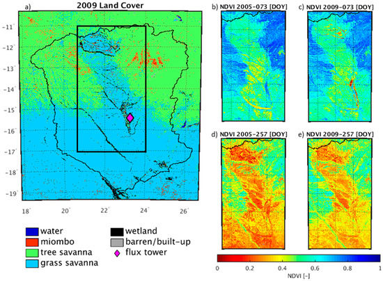
Figure 2.
Maps of the UZRB study region. (a) Land cover for 2009 derived from MODIS MCD12Q1 and simplified to represent southern Africa. The black rectangle shows the outline of the inset panels on the right side of the figure. (b–e) The Normalized Difference Vegetation Index (NDVI) for a wet (b,c) and dry (d,e) period in 2005 and 2009 showing the variability in vegetation around the wetlands. NDVI was derived from the MODIS MCD43B4 data as described in Section 2.3.1. The ZM-Mon (Mongu, Zambia) CarboAfrica site location is displayed.
The UZRB’s diverse ecosystems ranges from wet and dry miombo forest in the northern mountains to savanna and grassland in the south, in accordance with the latitudinal transition from humid to semi-arid and arid regional climate. Wet miombo comprises dry evergreen forest, swamp forest, evergreen riparian forest, and wet dambos (shallow wetlands) and occurs where mean annual precipitation exceeds 1000 mm/year, while dry miombo occurs where annual rainfall is below 1000 mm/year and consists of dry deciduous forest, deciduous riparian forest, and dry dambos [33]. The wet miombo also tends to have higher canopy heights, around 15 m tall. There is high spatial variability in regional vegetation as seen by damp forests and grasslands growing only kilometers away from dry badlands, which reflects large spatial variability in precipitation as well as in hydrogeology and surface–groundwater interactions. Natural and anthropogenic burning are prevalent in this region. The intensity and frequency of fires determines species prevalence as certain types of miombo are more sensitive or resistant to fires, and a dynamic relationship exists in the development of successive tree canopies that then control the effects of fire [34]. The dominant ecosystems in the UZRB exhibit spatial heterogeneity that reflects topographic and rainfall gradients. The MODIS yearly land cover product (MCD12Q1) over the region shows that wetlands develop preferentially in low-lying convergence zones where dynamical interactions among hydrological and ecohydrological processes, including surface–groundwater interactions, are most vigorous.
The annual rainfall, which increases with altitude and latitude, ranges from around 200 mm in a dry year in the southernmost part of the UZRB to 1400–1600 mm in the northwest around the AHP. The altitude-latitude rainfall patterns are governed by the migration of major climate boundaries. The Benguela ocean current flows northward along the western coast of Africa and creates dry conditions along the coast of Angola. The ITCZ shifts northward during the dry season (July/August) and southward during the wet season (January) and the CABZ separates easterly and westerly flows and corresponds to a moist, thermally unstable air mass that delivers heavy rainfall to the region [35]. The Angola Low pressure center falls over the Angola highlands during the wet season and is associated with heavy rainfall in Southern Africa [36]. During the wet season, the presence of the ITCZ, CABZ, and the Angolan Low in the vicinity of the study region controls rainfall delivery within the UZRB [37]. Inter-annual variability in the relative positions of these boundary zones during the wet season can have huge impacts on spatial and temporal precipitation distributions [36]. Further, the presence of the CABZ extends the rainy season in the area around the AHP once the ITCZ moves northward [38].
2.2. Data
2.2.1. Land Surface Properties
The MODIS MCD43B4 Aqua and Terra combined Nadir BRDF-Adjusted Reflectance (NBAR) product corrected for sun and view angle effects was used to generate a dynamic wetland dataset for the UZRB [39]. These data are available at a 1 km spatial and 8-day temporal resolution with seven wavebands in the infrared and visible ranges of the electromagnetic radiation spectrum (Table 1). Other data sets include the quality control product, MODIS MCD43B2, at the same spatial and temporal resolutions [40], and land cover classes following the International Geosphere-Biosphere Programme (IGBP) system, MODIS MCD12Q1 land cover type product [41]. The land cover data is a stationary product available for each year from 2002 to 2013 at 500 m resolution. Vegetation phenology information retrieved from the MODIS Terra MOD15A2 product provides Fraction of Photosynthetically Active Radiation (FPAR) and Leaf Area Index (LAI) reconstructed from surface reflectance also at 1 km resolution every 8 days [42]. Finally, the MODIS MOD17A2 GPP product (version 55) was obtained for comparison against model results [43].

Table 1.
MODIS instrument specifications and tasseled cap coefficients from [44].
All MODIS data products were projected into Universal Transverse Mercator using the MODIS Reprojection Tool [45]. Except for MOD17A2 GPP which is already corrected for cloud contamination, the non-static data were then gap-filled, cloud corrected and smoothed using a Savitzy-Golay filter in TIMESAT [46]. The static MCD12Q1 land cover data were spatially interpolated using a nearest neighbor algorithm to the same 1 km grid as the MCD43B4 data before selecting the training data. FPAR and LAI data were interpolated to the 5 km and 1-h resolution of the DCHM-V (Duke Coupled Hydrology Model with Vegetation).
2.2.2. Meteorological Forcing and Ancillary Data
Atmospheric forcing datasets were acquired for modeling purposes from the European Centre for Medium-Range Weather Forecasts (ECMWF) meteorological reanalysis data (ERA-Interim) available at 6-h intervals at 0.703° [47]. These data include air temperature, air pressure, wind velocity, specific humidity, and downward shortwave and long wave radiation. Precipitation accumulation data were provided at 3-h and ~25 km resolution by the Tropical Rainfall Measuring Mission (TRMM) 3B42 version 7 and instantaneous vertical rainfall profiles from TRMM 2A25 at 5 km horizontal and 250 m vertical resolution [48]. All forcing data were interpolated to the 5 km and 1-h model resolution using nearest neighbor.
Temporally invariant (ancillary) data are used to determine regional soil characteristics. Soil texture for the study area was extracted from the Harmonized World Soil Database at 30 arc sec spatial resolution [49]. The soil texture map was spatially interpolated using nearest neighbor to the 5 km model resolution. Soil parameters corresponding to saturated hydraulic conductivity, porosity, field capacity, and wilting point were determined from a look-up table based on the soil texture data [50,51,52].
2.3. Wetland Probability Mapping Algorithm
Wetland probability maps were created using a logistic regression model that combines indices derived from the surface reflectance data that are sensitive to surface greenness and water content. The model was trained on the MODIS MCD12Q1 IGBP land cover classes over a three-year window (2010–2012). All indices were derived from the MODIS MCD43B4 NBAR surface reflectance data. The indices and logistic regression model are described here. Identification of flooded areas by way of building indices from MODIS reflectance data has been used previously [32,53]; however, here we build off of the methodology developed by [32] and evaluate the effectiveness of individual indices before building the regression model.
2.3.1. NIR and NDVI
The near-infrared (NIR) band is represented by wavelengths between 841 nm and 876 nm on the MODIS instrument. This waveband is centered on a non-absorptive region in the water vapor spectra that minimizes interference (i.e., absorption) by atmospheric water vapor and allows for remote sensing of land surface reflectance [54,55]. The reflectance of NIR increases during vegetation growing seasons [56], tracing the plant life cycle [57]. This occurs because chlorophyll contained in leaves reflects near-infrared light, while absorbing visible red light. These properties are exploited in the NDVI, a measurement of greenness that represents a combination of vegetation properties, including leaf chlorophyll content, leaf area, structure, and canopy cover. NDVI is a ratio that returns index values between −1 and 1. Reflectance data from the MODIS instrument (specifications listed in Table 1) were used to calculate NDVI with the following equation [58]:
Generally, values of NDVI ranging from 0.30 to 1.00 indicate vegetation, with higher values corresponding to greener areas. Negative values and low, positive values represent water and different soils, respectively [59]. NDVI is more sensitive to vegetation cover than it is to bare soil characteristics, but its calculation does not completely remove the effects of background soil reflectance [60].
2.3.2. NDWI
The Normalized Difference Water Index (NDWI) measures surface water content based on the spectral reflectance properties of water [61]. There are various ways to calculate NDWI using a combination of visible green, near-infrared, or mid-infrared wavelengths. We use a modified NDWI equation proposed by [62] that emphasizes open water features by utilizing the visible green and mid-infrared reflectance bands [61]:
Since water reflects visible green light and absorbs mid-infrared wavelengths, NDWI values above or equal to 0 correspond to water, while negative values represent non-water surfaces [62]. This index is effective in reducing vegetation, soil, and built-up land noise, but may provide slight overestimates in water content [61].
2.3.3. Tasseled Cap Transformation
The Tasseled Cap (TC) transformation separates spectral features in MODIS NBAR reflectance data that relate to different land surface properties. The transformation consists of a principal component analysis performed on the MODIS NBAR data to define initial axes, and then subsequent rotations to separate non-vegetated, vegetated, and water and snow features [63]. The rotated components are expressed as a linear combination of the seven reflectance bands with weights as defined in Table 1:
where x corresponds to either brightness (b), greenness (g) or wetness (w).
The first set of coefficients developed from the TC transformation define the TC Brightness index and are sensitive to changes in total reflectance, as well as physical properties influencing total reflectance [63,64]. Based on a sensitivity analysis, soil variability is unambiguous, but differences in vegetation density do not greatly alter TC Brightness [64]. Index values are positive, ranging from 0 to around 0.75. Values closer to 0 correspond to water and/or barren areas, while values in the mid- to upper range characterize savanna regions; forests and cropland are represented throughout the entire range of values [63].
The second set of coefficients resulting from the TC transformation corresponds to the TC Greenness index (Table 1). The TC Greenness index is the difference between the sum of visible bands and near-infrared bands. Similarly to NDVI, TC Greenness is responsive to both high absorption in the visible bands and high reflectance in the near-infrared bands because of plant pigments and cellular leaf structure, respectively [64]. Higher greenness values represent greater densities of green vegetation, while lower greenness values generally correspond to water and soils.
The third rotated component is the TC Wetness index calculated as the difference between the sum of visible and near-infrared bands and longer infrared bands. The third set of coefficients derived from the TC transformation represents this wetness index (Table 1). In this calculation, longer infrared bands are suggested to be most sensitive to soil and plant moisture, with soil moisture status as the primary characteristic. Variation in plant moisture has limited representation in TC wetness [64]. The TC Wetness index yields negative values; those closest to 0 indicate the presence of bodies of water, while negative values farther away from 0 characterize a moisture gradient in which an increase in the magnitude of the index value generally corresponds to a decrease in moisture [63].
2.3.4. Logistic Regression Model for Probability Mapping
The logistic regression model describes how predictor variables relate to the binary dependent responses of wetland or non-wetland. In this case, the predictor variables are the indices described above. The Bernoulli response is modeled as:
where and describes the probability of wetland presence within a given pixel based on the predictors X. The regression coefficients serve as weights for each of the predictor variables that describe their relative contribution to the outcome probability. The nonlinear probability is transformed to a generalized linear model with a binomial distribution and logit-link function (Equation (4)). The logit transformation maps the probability from (0, 1) to (−, +) and allows for explicit calculation of the probability of event success.
The weights for the logistic regression model were determined from a training period comprised of three consecutive hydrologic wet years (2010 to 2012). First, a stationary land cover map was generated by removing pixels that varied in land cover type over the three-year period (Figure 3a). This stationary map was used to determine the fixed Bernoulli response values (i.e., wetland pixel = 1 and non-wetland pixel = 0). The resulting training pixels are summarized in Table 2. In the training data, the predictor variables (i.e., indices calculated from MODIS NBAR) were selected from the rainy seasons only (21 March–6 April) for training pixels randomly sampled from within the UZRB study region. Several models were trained using different combinations of indices. Once the weights were determined from the training data, the logistic regression model was applied to generate independent probability maps of wetlands every 8 days.
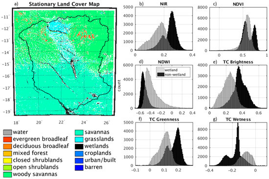
Figure 3.
Stationary land cover map and histograms for unitless remote sensing indices using only the pixels representing wetland and non-wetland in the training data. Stationary land cover data and indices were derived from the MODIS MCD12Q1 and MCD43B4, respectively. (a) Stationary land cover map derived from MODIS MCD12Q1 data for 2010–2012. (b–g) Histograms for wetland and non-wetland pixels using NIR (b), NDVI (c), NDWI (d), TC Brightness (e), TC Greenness (f) and TC Wetness (g).
Table 2.
Summary of training pixels (28,000 total) for each MODIS land cover type.
The best predictors for the linear regression model are those where there are clear differences in index values for wetland and non-wetland pixels. This can be observed in histograms of the indices that show isolated peaks for wetland and non-wetland pixels (Figure 3). The histograms represent moist conditions because the training data were obtained from only the rainy season. Thus, for a dry period the resulting histograms could be drastically different. Individually, NIR, NDWI, TC Brightness and TC Wetness show the clearest separations between wetland and non-wetland pixels. Using combinations of these indices in the logistic regression model will help remove the overlapping effects observed in the individual histograms.
2.3.5. Calculating Wetland Fractions
In order to compute wetland fractions at a given spatial scale, a threshold was determined to transform wetland probabilities into a binary signal for wetland presence. An area-threshold analysis was used to determine a cut-off probability above which we assume the 1 km pixel is completely covered by wetlands (Figure 4). Different probability thresholds were used to determine wetland presence at 1 km. We then calculated the area of the wetland extent over the entire UZRB basin at each threshold during the period of maximum wetland extent for a given year (around 9 April). The respective areas were compared to the wetland area determined by the stationary land cover map (Figure 3). Through this analysis, a threshold of 70% was determined to best represent the presence of wetlands; that is pixels with wetland probabilities ≥70% were assigned the value 1 and pixels with wetland probability <70% were assigned the value 0. Maps of wetland fractions were then created by averaging over 5 × 5 pixel windows. The resulting wetland maps are described in Section 3.1.
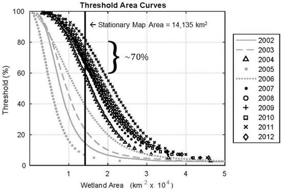
Figure 4.
Annual threshold-area curves used to determine how wetland probability corresponds to the presence of wetlands at the 1 km native resolution. The x-axis shows the maximal wetland area for the given probability threshold (y-axis). The vertical line indicates the wetland area from the stationary land cover map (Figure 2a). The years with extremely low wetland extents shown in gray were not used to determine the threshold. The remaining years range from 60–80% wetland probability to match the stationary wetland area. Stationary wetland area was derived from the MODIS MCD12Q1 data as described in Section 2.3.4.
2.4. Land-Surface Eco-Hydrology Modeling
The Duke Coupled Hydrology Model with Vegetation (DCHM-V) is used to investigate the impact of temporal changes in wetland extent on regional hydrology and plant productivity. It is a physically-based land-surface eco-hydrology model that consists of a mass balance to solve for soil moisture and water fluxes, an energy balance to solve for soil temperature and heat fluxes, physics for snow accumulation and melt, and a biochemical formulation of leaf photosynthesis [65,66,67,68,69,70,71,72,73,74,75]. In this study, the DCHM-V is implemented in 1-D where vertical energy and water fluxes are evaluated at each time step between the atmospheric boundary layer and 3 soil layers ranging from the surface to bedrock.
The DCHM-V simulates C3 and C4 photosynthetic pathways. The key difference in C3 and C4 photosynthesis is the existence of bundle sheath cells that allow for higher rates of carboxylation. The equations describing C4 photosynthesis within the DCHM-V are presented in Appendix A. It is assumed that all wetland, grassland and savanna vegetation undergo C4 photosynthesis [76], while all trees and shrubs (including miombo) undergo C3 photosynthesis [9,77]. When undergoing photosynthesis, wetlands are treated as savannas in order to determine biophysical properties.
2.5. Simulating Contributions of Wetlands to Water and Carbon Budgets
For the purposes of this study, the DCHM-V runs at 5 km spatial resolution and an hourly time-step. The wetland maps serve as a proxy for surface–groundwater interactions in the 1-D column model DCHM-V. When wetlands are present, vegetation in and around the inundated region have access to near-saturated, if not saturated, soil moisture. This added water source is able to sustain vegetation productivity past the wet season and allow for extended periods of carbon uptake well into the dry season. We use two simulations to evaluate how the presence of wetlands in the UZRB enhance fluxes of carbon and water between the land surface and the atmosphere. The first simulation uses the wetland maps to indicate where the pixels are fully inundated and soil moisture is fixed at saturation (WET). The second simulation assumes that wetlands are not present and soil moisture is controlled by evapotranspiration, infiltration, gravity, diffusion, and capillary action (DRY).
3. Results
3.1. Wetland Mapping
The temporally and spatially varying wetland maps demonstrate the inter-annual and inter-seasonal variability in wetland coverage not observed in the MODIS MCD12Q1 static land cover data (Figure 5 and Figure 6). The areal extent of wetlands in the MODIS product falls within the range of the minimum and maximum extent from the dynamic wetland maps, except for in 2005 which was an extremely dry year when the timing of wetland expansion appears to be controlled by groundwater contributions rather than seasonal rainfall (Figure 5). Deficits in groundwater estimated by the Gravity Recovery and Climate Experiment (GRACE) peak during the 2005 drought in the Zambezi basin and are associated with a large decrease in terrestrial water storage [32,78]. The annual variability in maximum wetland extent in Figure 5 follows the maximum observed discharge rates for the Zambezi River [79]. The spatial patterns of the maximum wetland area in the dynamic maps reflect the observed locations in the MODIS land cover data during the wet year (Figure 6). While in the dry year, the riparian wetlands observed in the MODIS data that are not present on the day of maximum wetland extent, but are observed over the course of the year (see Supplemental Materials Videos S1–S3).
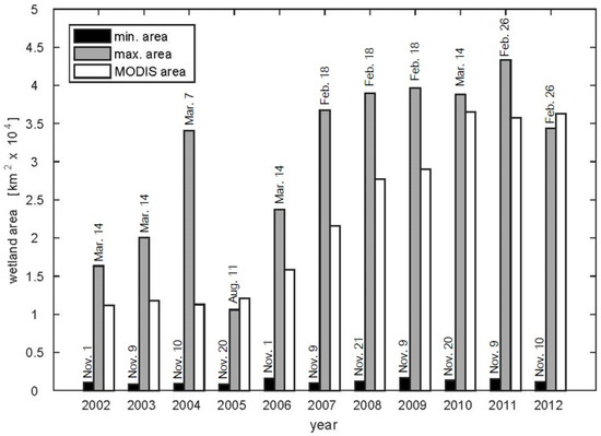
Figure 5.
Bar graph showing the annual variability in wetland area. The minimum (black) and maximum (gray) wetland areas for each year are displayed alongside the wetland area from the annual MODIS MCD12Q1 product (white). The dates for the minimum and maximum areal extents are displayed above their respective bars.
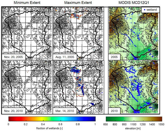
Figure 6.
Maps of wetland fractions for the days of minimum and maximum wetland extent displayed alongside the corresponding MODIS MCD12Q1 static wetland land cover class in 2005 and 2010. Topographic contours are displayed as black lines at every 100 m between 650 m and 1550 m.
3.2. Evaluation of C4 Photosynthesis Routine at Mongu, Zambia
The gross primary productivity (GPP) rates estimated by the C4 photosynthesis routine in the DCHM-V are evaluated against the MODIS MOD17A2 GPP product and eddy-covariance flux tower data collected at the ZM-Mon tower (Figure 7). The DCHM-V estimates compare well against the tower observations, particularly during the dry season and green-up periods. The MODIS GPP product severely underestimates both the DCHM-V and flux tower throughout most of the year, and by a difference of more than 5 g C/m2/day during the peak of the growing season, and it is not able to capture the variability in amplitude and overall seasonality of photosynthetic activity in this region. The fact that MODIS underestimates productivity in African savanna and grassland ecosystems has been documented previously and attributed to the uncertainties in incoming radiation, the insufficiency of vapor pressure deficit as an indicator of water stress in the MODIS algorithm, differences in spatial scale between MODIS pixels and flux tower footprints and subgrid heterogeneities (e.g., [80,81,82]). Thus, the remainder of the results and the discussion regarding carbon and water fluxes in the UZRB will focus on the DCHM-V and will not consider the MODIS data as a result of poor performance in this region.
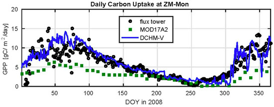
Figure 7.
Time series of daily GPP in 2008 from MODIS MOD17A2 (square), CarboAfrica flux tower data (circle), and the DCHM-V estimates at the same location. Note the significant difference between MOD17A2 and the DCHM-V estimates. The location of the ZM-Mon tower within the UZRB is shown in Figure 2.
3.3. Modeled Surface Fluxes
The results of the WET and DRY DCHM-V simulations indicate increases in ET and GPP for wetland areas (Figure 8). Overall, the presence of wetlands allows for higher ET fluxes with the largest increases during the driest months (May–October). During the wet season months, the differences in ET between WET and DRY simulations are smaller because the added water available in soils is minimal (Figure S2). Conversely, the additional soil moisture during the dry months do not translate to GPP in the WET simulations which show the lowest increases in GPP between July and September, because of higher ET, and thus lower water use efficiency.
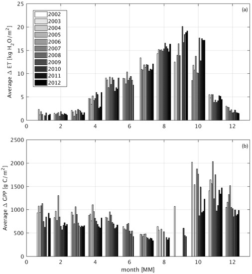
Figure 8.
Bar plots of the monthly difference in ET (a) and GPP (b) for all wetland pixels over the study period 2002 to 2012. Δ = WET − DRY. Each bar is normalized by the area of wetlands present. Dry season differences in July correspond to about 50% of GPP at ZM-Mon. Note the inverse trends of ET and GPP in the wet–dry transition season (April–July) vis-à-vis the dry–wet transition (September–December).
4. Discussion
4.1. Precipitation Gradients in the UZRB
A key land–atmosphere interaction in the UZRB is the growth of wetlands in response to precipitation gradients. We previously found that wetlands develop most fully between February and March in all years except 2005, which was an exceptionally dry year. Here the focus is on understanding how these areas recede during the dry season. In this region, March marks the end of the wet season and April serves as a transition period where infrequent and low rainfall accumulations are observed in “dry” years that tend to follow the elevation gradients (i.e., higher accumulations at higher elevations). In “wet” years, with high rainfall accumulations compared to the climatological average, large localized rainfall events occur in April and March in the midlands and lowlands of the basin that are not seen in “dry” years (Figure 9). For the following analysis, wet and dry years are distinguished by whether localized accumulations of rainfall are observed in the midland area in May. This means the period 2002–2006 defines dry years and 2007–2012 are wet years, in agreement with the hydrological drought observed in GRACE studies (e.g., [78]).
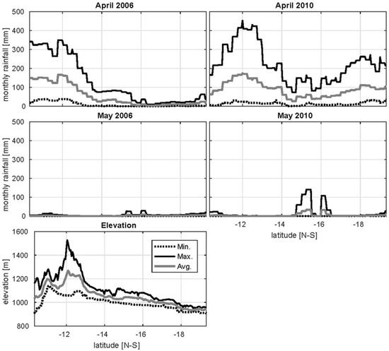
Figure 9.
Minimum, maximum, and mean monthly rainfall accumulations along a transect within the UZRB for April and May in a wet year (2006) and a dry (2010) year. The minimum, maximum, and average elevations along the transect positioned between 22.7° and 24° longitude are displayed.
4.2. Wetland Persistence and Dry Season Rainfall
The development of a spatially and temporally dynamic wetland classification in Section 2 permits an evaluation of wetland persistence under different wet and dry precipitation regimes. Wetland persistence is defined as the continuation of wetland areas past the onset of the dry season (i.e., May). The persistence of the UZRB midland wetlands is of particular interest due to the occurrence of localized rainfall events during wet years over this region (Figure 9, Figure S3). Dry years tend to have very low wetland persistence past the month of June (DOY 180, Figure 10 and Figure S3). The year 2004 shows an area around −15.25° latitude where 40–50% of the wetland area continues through August. This appears to be a case where remote groundwater contributions are playing a role, as there are no significant precipitation events occurring along this transect between May and August of 2004, and groundwater deficits nearly subside during the dry season in 2004 [78]. In wet years, high wetland fractions persist over large areas within the UZRB midlands (Figure 11, Figure S4).
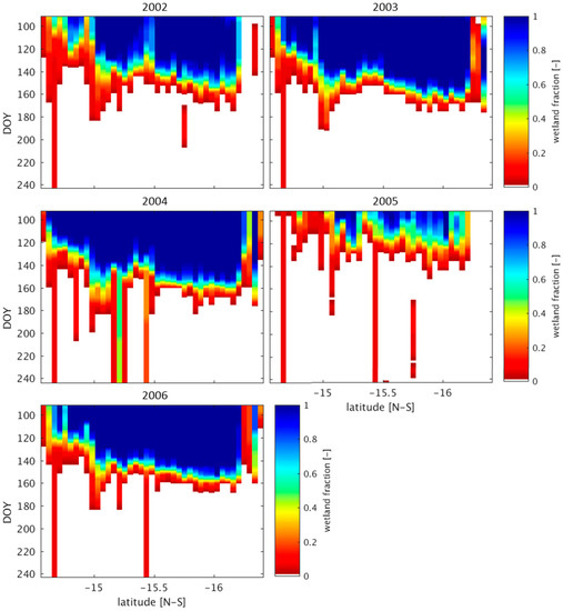
Figure 10.
Wetland persistence in dry years. These plots show the maximum wetland fraction along a transect located between 22.7° and 24° longitude. The subset area is displayed in Figure S1. In years 2002–2006 most wetland areas dry rapidly after the end of May (approximately day 150). Only very small areas persist until later in the dry season. Hövemöeller diagrams of rainfall in dry years over the same region are presented in Figure S3.
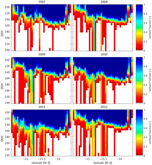
Figure 11.
Wetland persistence in wet years. These plots show the maximum wetland fraction along a transect located between 22.7° and 24° longitude. The subset area is displayed in Figure S1. In years 2007–2012 many wetland areas continue to exist after the end of May (approximately day 150), specifically between −15° and −15.5° latitude. Hövemöeller diagrams of rainfall in wet years over the same region are presented in Figure S4.
In order to better understand how the persistence of wetlands relates to localized rainfall events in the transition season, we evaluate the average diurnal cycles of local rainfall events around the midland wetlands. The rainfall accumulations from TRMM 3B42 consistently demonstrate a dual-peak in the diurnal cycle of rainfall in the early morning around 7–9 a.m. LST and in the afternoon between 5–8 p.m. LST in the transition season April–June (Figure 12, Figure S5). The bimodal diurnal pattern observed in the TRMM data is consistent with wet season low level cloud and fog formation patterns in the morning and late afternoon thunderstorms [83]. A word of caution is necessary to highlight the relatively coarse resolution of TRMM 3B42 at approximately 25 km2, which explains the very low rainfall rates per unit area in the diurnal cycle estimates (see also Figure S5). Further evaluation of these rainfall events using TRMM Precipitation Radar (PR) reflectivity (2A25 product) shows that the morning events are very shallow events with low reflectivity corresponding to radiation fog and low level clouds formed over the inundated areas in the early morning (Figure 13). Afternoon events correspond mostly to isolated shallow convection (<5 km height, not shown) with deeper convection features and higher intensity localized storms in the beginning of the transition season through early May (e.g., Video S4 for May 2009) as illustrated by the TRMM PR overpass example shown in Figure 13 for May 2008. Note the daily re-occurrence of isolated precipitation cells in the midland wetland region (highlighted by purple box in Figure S1). The TRMM 3B42 daily rainfall accumulations at approximately 25 × 25 km2 is relatively low, but the reflectivity profiles from TRMM 2A25 at 5 × 5 km2 suggest co-organization of individual afternoon rainfall cells and wetland pixels at high spatial resolution. This spatial organization over the wetland areas is similar to the classical model of cumulus development linked to high instability in the boundary-layer when the diurnal amplitude of Bowen ratio (sensible/latent heat fluxes) and the Bowen ratio proper are very small and near-surface relative humidity is high [84].
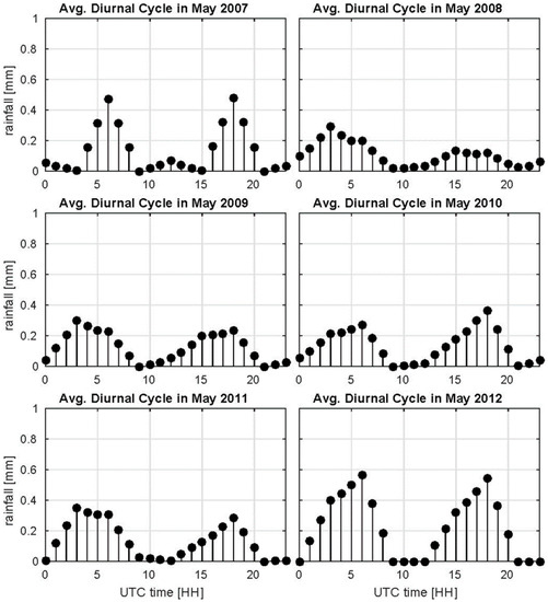
Figure 12.
Average diurnal cycle of TRMM 3B42 rainfall accumulations for the month of May. The diurnal cycle is marked by a bi-model precipitation pattern with peaks in morning and evening. Only pixels within the midland area marked by Figure S1 with monthly rainfall totals greater than 25 mm/month were considered for this analysis.
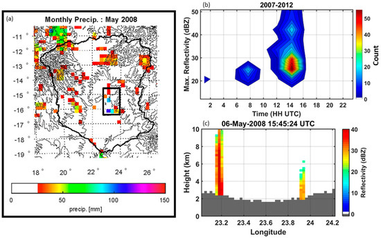
Figure 13.
Left panel (a) Cumulative monthly rainfall in May 2008 from TRMM 3B42 rainfall product (~25 km resolution). Black box indicates area of interest for land–atmosphere interactions and is the same area shown in Figure S1. Top right panel (b) Climatology of the diurnal cycle of rainfall reflectivity from TRMM PR 2A25 product (~5 km resolution) for the month of May. High reflectivity indicates high rainfall rates (i.e., intense storms events). These events only occur between 2007 and 2012. Bottom right panel (c) TRMM PR 2A25 reflectivity profiles as examples of isolated deep (early in the transition season) and shallow (daily) isolated convection at around 5:45 p.m. LST on 6 May 2008. The terrain cross-section is marked in dark gray.
Previous work demonstrated that moisture delivered to the atmosphere via plant evapotranspiration contributes up to 60% of energy available for convection along the eastern slopes of the Andes [85], which results in a decrease in precipitation up to 50% along the Andean slopes. Over the low-lying areas of the Amazon basin, the change in precipitation is on the order of 75%, where evapotranspiration is the dominant source of moisture [85,86]. Similarly, in a study on precipitation recycling in west Africa local evaporation served as the moisture source for 27% of local precipitation [87]. Figure 14 shows a conceptual illustration of the conditions favorable to develop land–atmosphere interactions in the UZRB consistent with observations. First, initial conditions that allow for regional wetland expansion are set by wet season precipitation linked to large scale forcing mostly at higher elevations in the AHP. Infiltration and groundwater recharge occur, followed by lateral redistribution by subsurface flows and discharge along the mid-basin low lying convergence areas. Second, rainfall recycling in the transition season (April–June) driven by up-valley daytime flows converging to the mid-basin region enhance cumulus convection locally, leveraging moist energy available from surface fluxes. Rainfall suppression in the dry season proper (July–September) reflect colder temperatures and depressed dew points with regard to morning fog, and the collapse of land–atmosphere interactions due to weakening of regional circulations, increased stability and reduced moisture supply. Thus, reductions in wetland extent in the UZRB limit the timing and amount of evapotranspiration and water vapor content in the lower troposphere, and in turn may impact low level stability and thus rainfall. The spatial and temporal scales over which this feedback between wetland persistence and local convective storms should be further investigated using a coupled land–atmosphere model.
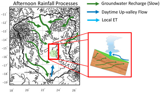
Figure 14.
Conceptual representation of land–atmosphere interactions driving the rainfall observed during the afternoon around the midland wetlands.
4.3. Impact of Wetlands on Productivity
It was previously shown that the presence and persistence of wetlands allowed for increases in ET and GPP in the UZRB. Water use efficiency (WUE) describes how efficiently vegetation uses water (ET) to undergo photosynthesis and fix atmospheric CO2 (GPP) and is defined as WUE = ET/GPP. WUE is computed for both the WET and DRY simulations (Figure 15). During the wet season (November–March), vegetation in the WET simulation is slightly more water use efficient. On the other hand, in the dry months WUE efficiency is much lower in the WET simulation compared to the DRY simulation. Wetland vegetation in the WET run has ready access to soil water and does not need to efficiently use water for photosynthesis. In the DRY simulation some effects of water scarcity are setting in forcing plants to be more efficient in their water usage during the dry season. This result aligns with previous findings that productivity of African grassland vegetation is highly sensitive to seasonal rainfall [88,89,90]. A limitation of this analysis is the inability to account for methane emissions from flooded areas [3,91]. Future work should evaluate how the seasonal and annual variability of wetland extent impact the overall carbon budget in the UZRB.
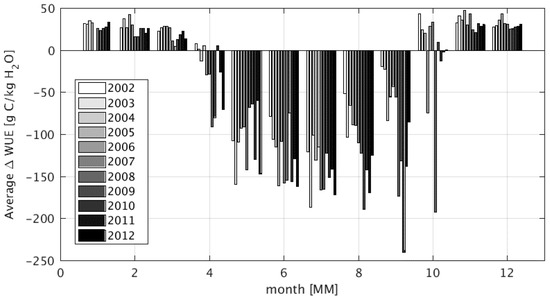
Figure 15.
Bar plots of the monthly difference in water use efficiency (WUE) for all wetland pixels over the study period 2002 to 2012. Δ = WET − DRY. Each bar is normalized by the area of wetlands present. Note that area of wetlands disappear at lower elevations in dry years, and thus the more efficient water use later in the dry season reflects the small areas of wetlands at higher elevations, colder temperatures, and where subsurface flow is the source of moisture. The water-use overhead of productivity increases nonlinearly through the dry season.
5. Conclusions
The co-variability of seasonal rainfall, wetland areal extent and how it impacts the coupled water–carbon cycles, and thus the UZRB carbon sink, was evaluated with a focus on wet-dry transition and dry season processes. The persistence of midland wetlands within the UZRB depends on localized rainfall events early in the dry season. The diurnal cycle of these events shows high intensity rainfall features in the afternoon and early evening. These findings suggest the potential for increased ET from wetlands to contribute as a moisture source for localized convective events, which should be evaluated further. The overall impacts of persistent wetlands corresponds to less efficient water use for photosynthesis during the wet season, but higher overall photosynthesis rates because wetland vegetation has unlimited access to water in soils. This work demonstrates the importance of wetlands in the UZRB in the coupled carbon and water budgets.
Supplementary Materials
The following are available online at http://www.mdpi.com/2072-4292/10/5/692/s1, Figure S1: Location of midland wetland areas used for analysis in Section 4 is highlighted in light purple, Figure S2: Bar plots of the monthly difference in soil moisture for all wetland pixels over the study period 2002 to 2012. Δ = WET − DRY. Each bar is normalized by the area of wetlands present, Figure S3: Hövemöeller diagrams of rainfall in dry years over the same region presented in Figure S1, Figure S4: Hövemöeller diagrams of rainfall in wet years over the same region presented in Figure S1, Figure S5: Average diurnal cycle of TRMM 3B42 rainfall accumulations for the month of May. The diurnal cycle is marked by a bi-model precipitation pattern with peaks in morning and evening. Only pixels within the midland area marked by Figure S1 with monthly rainfall totals greater than 25 mm/month were considered for this analysis. Note dual peaks in wet years in the early morning and in the afternoon, Video S1: Annual Wetland Classification from the MODIS MCD12Q1 Land Cover product. Location of wetlands are displayed over a digital elevation map from SRTM. Topographic contours are displayed as black lines at every 100 m between 650 m and 1550 m, Video S2: Wetland fractions corresponding to the 8-day MODIS retrieval periods for 2005 (dry year). Topographic contours are displayed as black lines at every 100 m between 650 m and 1550 m, Video S3: Wetland fractions corresponding to the 8-day MODIS retrieval periods for 2010 (wet year). Topographic contours are displayed as black lines at every 100 m between 650 m and 1550 m, Video S4: Daily rainfall accumulations during May 2009 using TRMM 3B42. Topographic contours are displayed as black lines at every 100 m between 650 m and 1550 m. The black box highlights the area of the midland wetlands.
Author Contributions
A.P.B. conceived the research. A.P.B. and L.E.L.L. designed the research plan. T.M.W. conducted the dynamic wetland classification and data analysis in collaboration with and guidance from L.E.L.L. L.E.L.L. implemented the DCHM-V in the UZRB. L.E.L.L. conducted and evaluated model simulations with guidance from A.P.B. L.E.L.L. and A.P.B. collaborated in data analysis, interpretation and paper writing.
Funding
This research was supported in part by the National Aeronautics and Space Administration under grant number NNX1616AL16G and the National Science Foundation under the award CNH1313799.
Acknowledgments
The MODIS MCD43B4, MCD43B2, MCD12Q1, MOD15A2 and MOD17A2 data products were retrieved from the online Data Pool, courtesy of the NASA Land Processes Distributed Active Archive Center (LP DAAC), USGS/Earth Resources Observation and Science (EROS) Center, Sioux Falls, South Dakota, https://lpdaac.usgs.gov/data_access/data_pool. Atmospheric forcing and ancillary datasets for the model simulations were prepared originally by Jing Tao while a research assistant in the Barros group.
Conflicts of Interest
The authors declare no conflict of interest. The founding sponsors had no role in the design of the study; in the collection, analyses, or interpretation of data; in the writing of the manuscript, and in the decision to publish the results.
Appendix A. C4 Photosynthesis Equations for DCHM-V
Appendix A.1. Overview
The DCHM-V models photosynthesis under a biochemical framework where it is assumed that the rate of carbon assimilation scales with the rates of key processes in the light and Calvin cycles. Photosynthesis is limited by either Rubisco activity or RuBP regeneration. Rubisco (ribulose-1,5-bisphosphate carboxylase/oxygenase) is the enzyme that catalyzes the reaction between RuBP (ribulose-1,5-bisphosphate) and atmospheric CO2 beginning the process of carbon fixation and ultimately the conversion of CO2 to sugars. C3 photosynthesis is called as such because this first step, known as the Photosynthetic Carbon Reduction (PCR) cycle, results in a three-carbon compound, phosphoglycerate (3-PGA). However, Rubisco catalyzes two competing processes: (1) Carboxylation through which carbon is converted to sugars, and (2) oxygenation, where oxygen is added to RuBP creating phosphoglycolate which serves no metabolic purpose and is toxic at high concentrations [92]. Processing phosphoglycolate requires photorespiration which is energy demanding and results in a loss of 25–30% fixed carbon [93]. C4 photosynthesis overcomes this limitation by spatially separating the sites of CO2 fixation and assimilation, thus suppressing the oxygenase activity of RuBP. Reducing the need for photorespiration means a more efficient use of CO2 for C4 plants.
C4 plants accomplish more efficient carbon assimilation through the evolutionary adaptation of a bundle sheath cell. Unlike in C3 photosynthesis where carbon fixation and assimilation both occur in the Mesophyll cell, in C4 photosynthesis CO2 is converted into a four-carbon organic acid (i.e., C4) through carboxylation of phosphoenolpyruvate (PEP) by PEP-carboxylase (PEPc). The C4 compounds are then sent to the bundle sheath cells and decarboxylated to release CO2. In the bundle sheath cells, Rubisco interacts with CO2 and forms the 3-PGA as part of the PCR cycle. Thus, a biochemical model for C4 photosynthesis must account for the limiting effects of both Rubisco and PEPc kinetics under light-saturated conditions.
Appendix A.2. C4 Photosynthesis Model Equations
Biochemical modeling of C4 photosynthesis follows from the methods developed for C3 photosynthesis. Key processes that limit photosynthetic activity are identified and represented as a Michaelis–Menten kinetics model. In C4 plants, these limiting processes include rate of electron transport (J) and Rubisco carboxylation (Ac), as seen in C3 photosynthesis, with the addition of the rate of PEP carboxylation (Vp). Net photosynthesis is assumed to be the minimum of the carboxylation rate () and the RuBP regeneration ().
The equations for and are presented below. The model variables and parameters are summarized in Table A1 and Table A2, respectively.
Appendix A.2.1. Carboxylation Equations
Carboxylation rate [94]:
Rate of PEP carboxylation [94]:
Rate of Rubisco carboxylation at high irradiance [94]:
Photorespiratory Compensation Point [94]:
Appendix A.2.2. RuBP Regeneration/Election Transport Rate Equations
Rate of RuBP regeneration under drying conditions [94]. Dry conditions correspond to less than 6.5% soil moisture in the median layer where most roots are located.
Rate of RuBP regeneration under wet conditions [94]:
Appendix A.2.3. Temperature Dependencies for Maximum Enzymatic Rates
Maximum enzymatic rates (i.e., , , and ) [95]:
Michaelis–Menten constants (, , ) [95]:
Table A1.
C4 Photosynthesis Model Variables in DCHM-V.
Table A1.
C4 Photosynthesis Model Variables in DCHM-V.
| Model Variable | Description | Units |
|---|---|---|
| Net carbon assimilation rate | mol C m−2 s−1 | |
| RuBP regeneration rate | mol C m−2 s−1 | |
| Carboxylation rate | mol C m−2 s−1 | |
| Rate of PEP carboxylation | mol C m−2 s−1 | |
| Rate of Rubisco carboxylation at high irradiance | mol C m−2 s−1 | |
| Maximum rate of carboxylation by Rubisco | mol C m−2 s−1 | |
| Michaelis–Menten constant for PEP carboxylase of CO2 | ubar | |
| Maximum rate of carboxylation by PEP | mol C m−2 s−1 | |
| Maximum rate of electron transport | mol C m−2 s−1 | |
| CO2 compensation point in bundle sheath cells | mol mol−1 | |
| Bundle-sheath CO2 partial pressure | unity | |
| Bundle-sheath O2 partial pressure | unity | |
| Rate of electron transport in mesophyll cells | mol C m−2 s−1 | |
| Rate of electron transport in bundle sheath cells | mol C m−2 s−1 | |
| Total rate of electron transport | mol C m−2 s−1 |
Table A2.
C4 Photosynthesis Model Parameters in DCHM-V.
Table A2.
C4 Photosynthesis Model Parameters in DCHM-V.
| Model Parameter | Description | Value | Units | Reference |
|---|---|---|---|---|
| Bundle sheath conductance | 3 | mmol m−2 s−1 | [96] | |
| CO2 concentration in mesophyll cell | mol m−3 | [67] | ||
| CO2 concentration outside the leaf boundary layer | 0.0145 | mol m−3 | [67] | |
| Mesophyll mitochondrial respiration | umol C m−2 s−1 | [94] | ||
| Leaf mitochondrial respiration | umol C m−2 s−1 | [94] | ||
| PEP regeneration rate | 80 | umol C m−2 s−1 | [94] | |
| Intercellular O2 concentration | 210 | mmol mol−1 | [97] | |
| Partitioning factor of electron transport rate | 0.4 | unity | [94] | |
| Half of reciprocal of Rubisco specificity | 0.000193 | unity | [94] |
Table A3.
C4 Photosynthesis Temperature Response Parameters (with standard errors).
Table A3.
C4 Photosynthesis Temperature Response Parameters (with standard errors).
| Parameter | Units | Measured at 25 °C | [umol m−2 s−1] | [kJ mol−1] | [kJ mol−1 K−1] | [kJ mol−1] | Reference |
|---|---|---|---|---|---|---|---|
| Kp | Pa CO2 | 16.0 ± 1.3 | 13.9 ± 1.0 | 36.3 ± 2.4 | - | - | [95] |
| μM HCO3 | 62.8 ± 5.0 | 60.5 ± 2.4 | 27.2 ± 2.8 | - | - | [95] | |
| Kc | Pa CO2 | 94.7 ± 15.1 | 121 ± 7 | 64.2 ± 4.5 | - | - | [95] |
| Ko | kPa of oxygen | 28.9 ± 5.4 | 29.2 ± 1.9 | 10.5 ± 4.8 | - | - | [95] |
| Sc/o | Pa/Pa | 1610 ± 66 | 1310 ± 52 | −31.1 ± 2.9 | - | - | [95] |
| Vpmax | μmol HCO3/m2/s | 450 ± 16 | - | - | [95] | ||
| Normalized to 1 at 25 °C | 1 | 1.01 ± 0.07 | 94.8 ± 40.8 | 0.25 ± 0.12 | 73.3 ± 39.6 | [95] | |
| μmol/m2/s | - | 125 | 70,373 | 376 | 177,910 | [96] | |
| μmol/m2/s | - | 159.9 ± 6.8 | 175.2 ± 3.8 171.6 ± 1.0 2 | - | - | [98] | |
| Vcmax | Normalized to 1 at 25° | 0.96 ± 0.04 | 0.89 ± 0.05 | 78.0 ± 4.1 | - | - | [95] |
| μmol/m2/s | - | 32 | 67,294 | 472 | 144,568 | [96] | |
| mol/m2/s | - | 3.9 ± 0.3 | 100.6 ± 2.0 156.1 ± 1.4 2 | [98] | |||
| Jmax | μmol/m2/s | - | 191 | 77,900 | 627 | 191,929 | [96] |
1 measured between 0 and 12 °C; 2 measured between 18 and 42 °C.
References
- Zedler, J.B.; Kercher, S. WETLAND RESOURCES: Status, Trends, Ecosystem Services, and Restorability. Annu. Rev. Environ. Resour. 2005, 30, 39–74. [Google Scholar] [CrossRef]
- Winter, T.C. The vulnerability of wetlands to climate change: A hydrologic landscape perspective1. JAWRA J. Am. Water Resour. Assoc. 2007, 36, 305–311. [Google Scholar] [CrossRef]
- Zhuang, Q.; Melillo, J.M.; Kicklighter, D.W.; Prinn, R.G.; McGuire, A.D.; Steudler, P.A.; Felzer, B.S.; Hu, S. Methane fluxes between terrestrial ecosystems and the atmosphere at northern high latitudes during the past century: A retrospective analysis with a process-based biogeochemistry model. Glob. Biogeochem. Cycles 2004, 18. [Google Scholar] [CrossRef]
- Matthews, E.; Fung, I. Methane emission from natural wetlands: Global distribution, area, and environmental characteristics of sources. Glob. Biogeochem. Cycles 1987, 1, 61–86. [Google Scholar] [CrossRef]
- Djebou, D.C.S. Integrated approach to assessing streamflow and precipitation alterations under environmental change: Application in the Niger River Basin. J. Hydrol. Reg. Stud. 2015, 4, 571–582. [Google Scholar] [CrossRef]
- Hunt, R.J.; Walker, J.F.; Krabbenhoft, D.P. Characterizing hydrology and the importance of ground-water discharge in natural and constructed wetlands. Wetlands 1999, 19, 458–472. [Google Scholar] [CrossRef]
- Taylor, A.R.D.; Howard, G.W.; Begg, G.W. Developing wetland inventories in southern Africa: A review. Vegetatio 1995, 118, 57–79. [Google Scholar] [CrossRef]
- Rebelo, L.-M.; McCartney, M.P.; Finlayson, C.M. Wetlands of Sub-Saharan Africa: Distribution and contribution of agriculture to livelihoods. Wetl. Ecol. Manag. 2010, 18, 557–572. [Google Scholar] [CrossRef]
- Merbold, L.; Ardö, J.; Arneth, A.; Scholes, R.J.; Nouvellon, Y.; de Grandcourt, A.; Archibald, S.; Bonnefond, J.M.; Boulain, N.; Brueggemann, N.; et al. Precipitation as driver of carbon fluxes in 11 African ecosystems. Biogeosciences 2009, 6, 1027–1041. [Google Scholar] [CrossRef]
- Gondwe, B.R.N.; Hong, S.-H.; Wdowinski, S.; Bauer-Gottwein, P. Hydrologic Dynamics of the Ground-Water-Dependent Sian Ka’an Wetlands, Mexico, Derived from InSAR and SAR Data. Wetlands 2010, 30, 1–13. [Google Scholar] [CrossRef]
- Lang, M.W.; Kasischke, E.S. Using C-Band Synthetic Aperture Radar Data to Monitor Forested Wetland Hydrology in Maryland’s Coastal Plain, USA. IEEE Trans. Geosci. Remote Sens. 2008, 46, 535–546. [Google Scholar] [CrossRef]
- Lee, H.; Beighley, R.E.; Alsdorf, D.; Jung, H.C.; Shum, C.K.; Duan, J.; Guo, J.; Yamazaki, D.; Andreadis, K. Characterization of terrestrial water dynamics in the Congo Basin using GRACE and satellite radar altimetry. Remote Sens. Environ. 2011, 115, 3530–3538. [Google Scholar] [CrossRef]
- Marechal, C.; Pottier, E.; Allain-Bailhache, S.; Meric, S.; Hubert-Moy, L.; Corgne, S. Mapping dynamic wetland processes with a one year RADARSAT-2 quad pol time-series. In Proceedings of the 2011 IEEE International Geoscience and Remote Sensing Symposium, Vancouver, BC, Canada, 24–29 July 2011; pp. 126–129. [Google Scholar]
- Milzow, C.; Krogh, P.E.; Bauer-Gottwein, P. Combining satellite radar altimetry, SAR surface soil moisture and GRACE total storage changes for hydrological model calibration in a large poorly gauged catchment. Hydrol. Earth Syst. Sci. 2011, 15, 1729–1743. [Google Scholar] [CrossRef]
- O’Grady, D.; Leblanc, M.; Bass, A. The use of radar satellite data from multiple incidence angles improves surface water mapping. Remote Sens. Environ. 2014, 140, 652–664. [Google Scholar] [CrossRef]
- Papa, F.; Prigent, C.; Rossow, W.B.; Legresy, B.; Remy, F. Inundated wetland dynamics over boreal regions from remote sensing: The use of Topex-Poseidon dual-frequency radar altimeter observations. Int. J. Remote Sens. 2006, 27, 4847–4866. [Google Scholar] [CrossRef]
- Sass, G.Z.; Creed, I.F. Characterizing hydrodynamics on boreal landscapes using archived synthetic aperture radar imagery. Hydrol. Process. 2008, 22, 1687–1699. [Google Scholar] [CrossRef]
- Landmann, T.; Schramm, M.; Colditz, R.R.; Dietz, A.; Dech, S. Wide Area Wetland Mapping in Semi-Arid Africa Using 250-Meter MODIS Metrics and Topographic Variables. Remote Sens. 2010, 2, 1751–1766. [Google Scholar] [CrossRef]
- Schroeder, R.; Rawlins, M.A.; McDonald, K.C.; Podest, E.; Zimmermann, R.; Kueppers, M. Satellite microwave remote sensing of North Eurasian inundation dynamics: Development of coarse-resolution products and comparison with high-resolution synthetic aperture radar data. Environ. Res. Lett. 2010, 5, 015003. [Google Scholar] [CrossRef]
- Baker, C.; Lawrence, R.L.; Montagne, C.; Patten, D. Change detection of wetland ecosystems using landsat imagery and change vector analysis. Wetlands 2007, 27, 610–619. [Google Scholar] [CrossRef]
- Baker, C.; Lawrence, R.; Montagne, C.; Patten, D. Mapping wetlands and riparian areas using landsat etm+ imagery and decision-tree-based models. Wetlands 2006, 26, 465–474. [Google Scholar] [CrossRef]
- Johnston, R.M.; Barson, M.M. Remote sensing of Australian wetlands: An evaluation of Landsat TM data for inventory and classification. Mar. Freshw. Res. 1993, 44, 235–252. [Google Scholar] [CrossRef]
- Davranche, A.; Lefebvre, G.; Poulin, B. Wetland monitoring using classification trees and SPOT-5 seasonal time series. Remote Sens. Environ. 2010, 114, 552–562. [Google Scholar] [CrossRef]
- Harvey, K.R.; Hill, G.J.E. Vegetation mapping of a tropical freshwater swamp in the Northern Territory, Australia: A comparison of aerial photography, Landsat TM and SPOT satellite imagery. Int. J. Remote Sens. 2001, 22, 2911–2925. [Google Scholar] [CrossRef]
- Akumu, C.E.; Pathirana, S.; Baban, S.; Bucher, D. Monitoring coastal wetland communities in north-eastern NSW using ASTER and Landsat satellite data. Wetl. Ecol. Manag. 2010, 18, 357–365. [Google Scholar] [CrossRef]
- Pantaleoni, E.; Wynne, R.H.; Galbraith, J.M.; Campbell, J.B. A logit model for predicting wetland location using ASTER and GIS. Int. J. Remote Sens. 2009, 30, 2215–2236. [Google Scholar] [CrossRef]
- Pantaleoni, E.; Wynne, R.H.; Galbraith, J.M.; Campbell, J.B. Mapping wetlands using ASTER data: A comparison between classification trees and logistic regression. Int. J. Remote Sens. 2009, 30, 3423–3440. [Google Scholar] [CrossRef]
- Campos, J.C.; Sillero, N.; Brito, J.C. Normalized difference water indexes have dissimilar performances in detecting seasonal and permanent water in the Sahara–Sahel transition zone. J. Hydrol. 2012, 464–465, 438–446. [Google Scholar] [CrossRef]
- Jain, S.K.; Singh, R.D.; Jain, M.K.; Lohani, A.K. Delineation of Flood-Prone Areas Using Remote Sensing Techniques. Water Resour. Manag. 2005, 19, 333–347. [Google Scholar] [CrossRef]
- Adam, E.; Mutanga, O.; Rugege, D. Multispectral and hyperspectral remote sensing for identification and mapping of wetland vegetation: A review. Wetl. Ecol. Manag. 2010, 18, 281–296. [Google Scholar] [CrossRef]
- Ozesmi, S.L.; Bauer, M.E. Satellite remote sensing of wetlands. Wetl. Ecol. Manag. 2002, 10, 381–402. [Google Scholar] [CrossRef]
- Tao, J. Understanding the Coupled Surface-Groundwater System from Event to Decadal Scale Using an Un-Calibrated Hydrologic Model and Data Assimilation. Ph.D. Thesis, Duke University, Durham, NC, USA, 2015. [Google Scholar]
- Desanker, P.V.; Prentice, I.C. MIOMBO—A vegetation dynamics model for the miombo woodlands on Zambezian Africa. For. Ecol. Manag. 1994, 69, 87–95. [Google Scholar] [CrossRef]
- Lawton, R.M. A Study of the Dynamic Ecology of Zambian Vegetation. J. Ecol. 1978, 66, 175–198. [Google Scholar] [CrossRef]
- Nicholson, S.E.; Dezfuli, A.K.; Klotter, D. A Two-Century Precipitation Dataset for the Continent of Africa. Bull. Am. Meteorol. Soc. 2012, 93, 1219–1231. [Google Scholar] [CrossRef]
- Tazalika, L.; Jury, M.R. Intra-seasonal rainfall oscillations over central Africa: Space-time character and evolution. Theor. Appl. Climatol. 2008, 94, 67–80. [Google Scholar] [CrossRef]
- Schefuß, E.; Kuhlmann, H.; Mollenhauer, G.; Prange, M.; Pätzold, J. Forcing of wet phases in southeast Africa over the past 17,000 years. Nature 2011, 480, 509–512. [Google Scholar] [CrossRef] [PubMed]
- Dupont, L.M.; Behling, H.; Kim, J.-H. Thirty thousand years of vegetation development and climate change in Angola (Ocean Drilling Program Site 1078). Clim. Past 2008, 4, 107–124. [Google Scholar] [CrossRef]
- NASA LP DAAC. MODIS MCD43B4 Nadir BRDF-Adjusted Reflectance; Version 5; USGS Earth Resources Observation and Science (EROS) Center: Sioux Falls, SD, USA. Available online: https://lpdaac.usgs.gov/dataset_discovery/modis/modis_products_table/mcd43b4 (accessed on 12 July 2017).
- NASA LP DAAC. MODIS MCD43B2 BRDF-Albedo Quality; Version 5; USGS Earth Resources Observation and Science (EROS) Center: Sioux Falls, SD, USA. Available online: https://lpdaac.usgs.gov/dataset_discovery/modis/modis_products_table/mcd12q1 (accessed on 12 July 2017).
- NASA LP DAAC. MODIS MCD12Q1 Land Cover Type; Version 51; USGS Earth Resources Observation and Science (EROS) Center: Sioux Falls, SD, USA. Available online: https://lpdaac.usgs.gov/dataset_discovery/modis/modis_products_table/mcd12q1 (accessed on 12 July 2017).
- NASA LP DAAC. MODIS MOD15A2 Leaf Area Index—Fraction of Photosynthetically Active Radiation; Version 5; USGS Earth Resources Observation and Science (EROS) Center: Sioux Falls, SD, USA. Available online: https://lpdaac.usgs.gov/dataset_discovery/modis/modis_products_table/mod15a2 (accessed on 12 July 2017).
- NASA LP DAAC. MODIS MOD17A2 Gross Primary Productivity; Version 55; USGS Earth Resources Observation and Science (EROS) Center: Sioux Falls, SD, USA. Available online: https://lpdaac.usgs.gov/dataset_discovery/modis/modis_products_table/mod17a2 (accessed on 12 July 2017).
- Lobser, S.E.; Cohen, W.B. MODIS tasselled cap: Land cover characteristics expressed through transformed MODIS data. Int. J. Remote Sens. 2007, 28, 5079–5101. [Google Scholar] [CrossRef]
- Dwyer, J.L.; Schmidt, G.L. The MODIS reprojection tool. In Earth Science Satellite Remote Sensing; Springer: Berlin/Heidelberg, Germany, 2006; pp. 162–177. [Google Scholar]
- Jönsson, P.; Eklundh, L. TIMESAT—A program for analyzing time-series of satellite sensor data. Comput. Geosci. 2004, 30, 833–845. [Google Scholar] [CrossRef]
- ERA-Interim Project. Available online: https://doi.org/10.5065/D6CR5RD9 (accessed on 1 July 2015).
- Huffman, G.J.; Bolvin, D.T.; Nelkin, E.J.; Wolff, D.B.; Adler, R.F.; Gu, G.; Hong, Y.; Bowman, K.P.; Stocker, E.F. The TRMM Multisatellite Precipitation Analysis (TMPA): Quasi-Global, Multiyear, Combined-Sensor Precipitation Estimates at Fine Scales. J. Hydrometeorol. 2007, 8, 38–55. [Google Scholar] [CrossRef]
- Fischer, G.; Nachtergaele, F.O.; Prieler, S.; van Velthuizen, H.T.; Verelst, L.; Wiberg, D. Global Agro-Ecological Zones Assessment of Agriculture in the 21st Century; International Instituefor Applied Systems Analysis: Laxenburg, Austria; FAO: Rome, Italy, 2008. [Google Scholar]
- Rawles, W.J.; Brakensiek, D.L. Estimating Soil Water Retention from Soil Properties. J. Irrig. Drain. Div. 1982, 108, 166–171. [Google Scholar]
- Rawls, W.J.; Gish, T.J.; Brakensiek, D.L. Estimating Soil Water Retention from Soil Physical Properties and Characteristics. In Advances in Soil Science; Advances in Soil Science; Springer: New York, NY, USA, 1991; pp. 213–234. ISBN 978-1-4612-7812-2. [Google Scholar]
- Rawls, W.J.; Ahuja, L.R.; Brakensiek, D.L.; Shirmohammadi, A. Infiltration and soil water movement. In Handbook of Hydrology; Maidment, R., Ed.; McGraw-Hill: New York, NY, USA, 1993. [Google Scholar]
- Di Vittorio, C.A.; Georgakakos, A.P. Land cover classification and wetland inundation mapping using MODIS. Remote Sens. Environ. 2018, 204, 1–17. [Google Scholar] [CrossRef]
- Kaufman, Y.J.; Gao, B.C. Remote sensing of water vapor in the near IR from EOS/MODIS. IEEE Trans. Geosci. Remote Sens. 1992, 30, 871–884. [Google Scholar] [CrossRef]
- Vermote, E.F.; El Saleous, N.Z.; Justice, C.O. Atmospheric correction of MODIS data in the visible to middle infrared: First results. Remote Sens. Environ. 2002, 83, 97–111. [Google Scholar] [CrossRef]
- Chen, D.; Huang, J.; Jackson, T.J. Vegetation water content estimation for corn and soybeans using spectral indices derived from MODIS near- and short-wave infrared bands. Remote Sens. Environ. 2005, 98, 225–236. [Google Scholar] [CrossRef]
- Liang, S.; Fang, H.; Chen, M.; Shuey, C.J.; Walthall, C.; Daughtry, C.; Morisette, J.; Schaaf, C.; Strahler, A. Validating MODIS land surface reflectance and albedo products: Methods and preliminary results. Remote Sens. Environ. 2002, 83, 149–162. [Google Scholar] [CrossRef]
- Huete, A.; Didan, K.; van Leeuwen, W.; Miura, T.; Glenn, E. MODIS Vegetation Indices. In Land Remote Sensing and Global Environmental Change: NASA’s Earth Observing System and the Science of ASTER and MODIS, Remote Sensing and Digital Image Processing; Springer: New York, NY, USA, 2011; p. 579. [Google Scholar]
- Valor, E.; Caselles, V. Mapping land surface emissivity from NDVI: Application to European, African, and South American areas. Remote Sens. Environ. 1996, 57, 167–184. [Google Scholar] [CrossRef]
- Li, Z.-L.; Becker, F. Properties and comparison of temperature-independent thermal infrared spectral indices with NDVI for HAPEX data. Remote Sens. Environ. 1990, 33, 165–182. [Google Scholar] [CrossRef]
- Xu, H. Modification of normalised difference water index (NDWI) to enhance open water features in remotely sensed imagery. Int. J. Remote Sens. 2006, 27, 3025–3033. [Google Scholar] [CrossRef]
- McFeeters, S.K. Using the Normalized Difference Water Index (NDWI) within a Geographic Information System to Detect Swimming Pools for Mosquito Abatement: A Practical Approach. Remote Sens. 2013, 5, 3544–3561. [Google Scholar] [CrossRef]
- Zhang, X.; Schaaf, C.B.; Friedl, M.A.; Strahler, A.H.; Gao, F.; Hodges, J.C.F. MODIS tasseled cap transformation and its utility. In Proceedings of the IEEE International Geoscience and Remote Sensing Symposium; Toronto, ON, Canada, 24–28 June 2002; Volume 2, pp. 1063–1065. [Google Scholar]
- Crist, E.P.; Cicone, R.C. A Physically-Based Transformation of Thematic Mapper Data—The TM Tasseled Cap. IEEE Trans. Geosci. Remote Sens. 1984, GE-22, 256–263. [Google Scholar] [CrossRef]
- Barros, A.P. Adaptive Multilevel Modeling of Land-Atmosphere Interactions. J. Clim. 1995, 8, 2144–2160. [Google Scholar] [CrossRef]
- Devonec, E.; Barros, A.P. Exploring the transferability of a land-surface hydrology model. J. Hydrol. 2002, 265, 258–282. [Google Scholar] [CrossRef]
- Garcia-Quijano, J.F.; Barros, A.P. Incorporating canopy physiology into a hydrological model: Photosynthesis, dynamic respiration, and stomatal sensitivity. Ecol. Model. 2005, 185, 29–49. [Google Scholar] [CrossRef]
- Gebremichael, M.; Barros, A. Evaluation of MODIS Gross Primary Productivity (GPP) in tropical monsoon regions. Remote Sens. Environ. 2006, 100, 150–166. [Google Scholar] [CrossRef]
- Yildiz, O.; Barros, A.P. Climate Variability, Water Resources, and Hydrologic Extremes—Modeling the Water and Energy Budgets. Clim. Hydrol. Mt. Areas 2006. [Google Scholar] [CrossRef]
- Yildiz, O.; Barros, A.P. Elucidating vegetation controls on the hydroclimatology of a mid-latitude basin. J. Hydrol. 2007, 333, 431–448. [Google Scholar] [CrossRef]
- Yıldız, O.; Barros, A.P. Evaluating spatial variability and scale effects on hydrologic processes in a midsize river basin. Sci. Res. Essays 2009, 4, 217–225. [Google Scholar]
- Tao, J.; Barros, A.P. The Integrated Precipitation and Hydrology Experiment—Hydrologic Applications for the Southeast US (IPHEx-H4SE) Part II: Atmospheric Forcing and Topographic Corrections; Duke University: Durham, NC, USA, 2014. [Google Scholar]
- Tao, J.; Barros, A.P. Coupled prediction of flood response and debris flow initiation during warm- and cold-season events in the Southern Appalachians, USA. Hydrol. Earth Syst. Sci. 2014, 18, 367–388. [Google Scholar] [CrossRef]
- Lowman, L.E.L.; Barros, A.P. Interplay of drought and tropical cyclone activity in SE U.S. gross primary productivity. J. Geophys. Res. Biogeosci. 2016, 121, 1540–1567. [Google Scholar] [CrossRef]
- Lowman, L.E.L.; Barros, A.P. Predicting canopy biophysical properties and sensitivity of plant carbon uptake to water limitations with a coupled eco-hydrological framework. Ecol. Model. 2018, 372, 33–52. [Google Scholar] [CrossRef]
- Skarpe, C. Plant functional types and climate in a southern African savanna. J. Veg. Sci. 1996, 7, 397–404. [Google Scholar] [CrossRef]
- Caylor, K.K.; Shugart, H.H. Simulated productivity of heterogeneous patches in Southern African savanna landscapes using a canopy productivity model. Landsc. Ecol. 2004, 19, 401–415. [Google Scholar] [CrossRef]
- Thomas, A.C.; Reager, J.T.; Famiglietti, J.S.; Rodell, M. A GRACE-based water storage deficit approach for hydrological drought characterization. Geophys. Res. Lett. 2014, 41, 1537–1545. [Google Scholar] [CrossRef]
- Jury, M.R. A return to wet conditions over Africa: 1995–2010. Theor. Appl. Climatol. 2013, 111, 471–481. [Google Scholar] [CrossRef]
- Sjöström, M.; Zhao, M.; Archibald, S.; Arneth, A.; Cappelaere, B.; Falk, U.; de Grandcourt, A.; Hanan, N.; Kergoat, L.; Kutsch, W.; et al. Evaluation of MODIS gross primary productivity for Africa using eddy covariance data. Remote Sens. Environ. 2013, 131, 275–286. [Google Scholar] [CrossRef]
- Sjöström, M.; Ardö, J.; Arneth, A.; Boulain, N.; Cappelaere, B.; Eklundh, L.; de Grandcourt, A.; Kutsch, W.L.; Merbold, L.; Nouvellon, Y.; et al. Exploring the potential of MODIS EVI for modeling gross primary production across African ecosystems. Remote Sens. Environ. 2011, 115, 1081–1089. [Google Scholar] [CrossRef]
- Jin, C.; Xiao, X.; Merbold, L.; Arneth, A.; Veenendaal, E.; Kutsch, W.L. Phenology and gross primary production of two dominant savanna woodland ecosystems in Southern Africa. Remote Sens. Environ. 2013, 135, 189–201. [Google Scholar] [CrossRef]
- Cohen, L.T.; Matos, J.P.; Boillat, J.-L.; Schleiss, A.J. Comparison and evaluation of satellite derived precipitation products for hydrological modeling of the Zambezi River Basin. Hydrol. Earth Syst. Sci. 2012, 16, 489–500. [Google Scholar] [CrossRef]
- Barros, A.P.; Hwu, W. A study of land-atmosphere interactions during summertime rainfall using a mesoscale model. J. Geophys. Res. Atmos. 2002, 107, ACL 17-1–ACL 17-18. [Google Scholar] [CrossRef]
- Sun, X.; Barros, A.P. Isolating the Role of Surface Evapotranspiration on Moist Convection along the Eastern Flanks of the Tropical Andes Using a Quasi-Idealized Approach. J. Atmos. Sci. 2014, 72, 243–261. [Google Scholar] [CrossRef]
- Sun, X.; Barros, A.P. Impact of Amazonian evapotranspiration on moisture transport and convection along the eastern flanks of the tropical Andes. Q. J. R. Meteorol. Soc. 2015, 141, 3325–3343. [Google Scholar] [CrossRef]
- Gong, C.; Eltahir, E. Sources of moisture for rainfall in West Africa. Water Resour. Res. 1996, 32, 3115–3121. [Google Scholar] [CrossRef]
- Zhu, L.; Southworth, J. Disentangling the Relationships between Net Primary Production and Precipitation in Southern Africa Savannas Using Satellite Observations from 1982 to 2010. Remote Sens. 2013, 5, 3803–3825. [Google Scholar] [CrossRef]
- Sankaran, M.; Hanan, N.P.; Scholes, R.J.; Ratnam, J.; Augustine, D.J.; Cade, B.S.; Gignoux, J.; Higgins, S.I.; Le Roux, X.; Ludwig, F.; et al. Determinants of woody cover in African savannas. Nature 2005, 438, 846–849. [Google Scholar] [CrossRef] [PubMed]
- Campo-Bescós, M.A.; Muñoz-Carpena, R.; Southworth, J.; Zhu, L.; Waylen, P.R.; Bunting, E. Combined Spatial and Temporal Effects of Environmental Controls on Long-Term Monthly NDVI in the Southern Africa Savanna. Remote Sens. 2013, 5, 6513–6538. [Google Scholar] [CrossRef]
- Melton, J.R.; Wania, R.; Hodson, E.L.; Poulter, B.; Ringeval, B.; Spahni, R.; Bohn, T.; Avis, C.A.; Beerling, D.J.; Chen, G.; et al. Present state of global wetland extent and wetland methane modelling: Conclusions from a model inter-comparison project (WETCHIMP). Biogeosciences 2013, 10, 753–788. [Google Scholar] [CrossRef]
- Gowik, U.; Westhoff, P. The Path from C3 to C4 Photosynthesis. Plant Physiol. 2011, 155, 56–63. [Google Scholar] [CrossRef] [PubMed]
- Lara, M.V.; Andreo, C.S. C4 Plants Adaptation to High Levels of CO2 and to Drought Environments. In Abiotic Stress in Plants-Mechanisms and Adaptations; IntechOpen: Hampshire, UK, 2011. [Google Scholar] [CrossRef]
- Von Caemmerer, S. Biochemical Models of Leaf Photosynthesis; CSIRO Publishing: Clayton, Australia, 2000. [Google Scholar]
- Boyd, R.A.; Gandin, A.; Cousins, A.B. Temperature Responses of C4 Photosynthesis: Biochemical Analysis of Rubisco, Phosphoenolpyruvate Carboxylase, and Carbonic Anhydrase in Setaria viridis. Plant Physiol. 2015, 169, 1850–1861. [Google Scholar] [CrossRef] [PubMed]
- Massad, R.-S.; Tuzet, A.; Bethenod, O. The effect of temperature on C4-type leaf photosynthesis parameters. Plant Cell Environ. 2007, 30, 1191–1204. [Google Scholar] [CrossRef] [PubMed]
- Medlyn, B.E.; Dreyer, E.; Ellsworth, D.; Forstreuter, M.; Harley, P.C.; Kirschbaum, M.U.F.; Le Roux, X.; Montpied, P.; Strassemeyer, J.; Walcroft, A.; et al. Temperature response of parameters of a biochemically based model of photosynthesis. II. A review of experimental data. Plant Cell Environ. 2002, 25, 1167–1179. [Google Scholar] [CrossRef]
- Kubien, D.S.; von Caemmerer, S.; Furbank, R.T.; Sage, R.F. C4 Photosynthesis at Low Temperature. A Study Using Transgenic Plants with Reduced Amounts of Rubisco. Plant Physiol. 2003, 132, 1577–1585. [Google Scholar] [CrossRef] [PubMed]


© 2018 by the authors. Licensee MDPI, Basel, Switzerland. This article is an open access article distributed under the terms and conditions of the Creative Commons Attribution (CC BY) license (http://creativecommons.org/licenses/by/4.0/).