Impact of Changes in Minimum Reflectance on Cloud Discrimination

Abstract

Greenhouse Gases Observing SATellite-2 (GOSAT-2) will be launched in fiscal year 2018. GOSAT-2 will be equipped with two Earth-observing instruments: the Thermal and Near-infrared Sensor for carbon Observation Fourier Transform Spectrometer 2 (TANSO-FTS-2) and TANSO-Cloud and Aerosol Imager 2 (CAI-2). CAI-2 can be used to perform cloud discrimination in each band. The cloud discrimination algorithm uses minimum reflectance (R_min) for comparisons with observed top-of-atmosphere reflectance. The creation of cloud-free R_min requires 10 CAI or CAI-2 data. Thus, R_min is created from CAI L1B data for a 30-day period in GOSAT, with a revisit time of 3 days. It is necessary to change the way in which 10 observations are chosen for GOSAT-2, which has a revisit time of 6 days. Additionally, R_min processing for GOSAT CAI data was updated to version 02.00 in December 2016. Along with this change, the resolution of R_min changed from 1/30° to 500 m. We examined the impact of changes in R_min on cloud discrimination results using GOSAT CAI data. In particular, we performed comparisons of: (1) R_min calculated using different methods to choose the 10 observations and (2) R_min calculated using different generation procedures and spatial resolutions. The results were as follows: (1) The impact of using different methods to choose the 10 observations on cloud discrimination results was small, except for a few cases, e.g., snow-covered regions and sun-glint regions; (2) Cloud discrimination results using R_min in version 02.00 were better than results obtained using R_min in the previous version, apart from some special situations. The main causes of this were as follows: (1) The change of used band from band 2 to band 1 for R_min calculation; (2) The change of spatial resolution of R_min from 1/30° to 500-m.

1. Introduction

Greenhouse gases Observing SATellite-2 (GOSAT-2) will be launched in fiscal year 2018. GOSAT-2 will be equipped with two Earth-observing instruments: the Thermal and Near-infrared Sensor for carbon Observation Fourier Transform Spectrometer 2 (TANSO-FTS-2) and the TANSO-Cloud and Aerosol Imager 2 (CAI-2). CAI-2 is a push-broom imaging sensor that has forward- and backward-looking bands (±20°) for observing the optical properties of aerosols and clouds and for monitoring the status of transboundary air pollution over oceans to avoid sun-glint. In contrast, the existing GOSAT TANSO-CAI obtains measurements at a fixed angle close to the nadir [1]. An important function of CAI-2 is cloud discrimination using each band to identify and reject cloud-contaminated FTS-2 data; the presence of clouds in the instantaneous field-of-view (IFOV) of FTS-2 leads to errors in estimates of atmospheric greenhouse gas concentrations. For GOSAT CAI L2 cloud flag products, the Cloud and Aerosol Unbiased Decision Intellectual Algorithm (CLAUDIA1) [2,3] is used. For GOSAT-2 CAI-2 L2 cloud discrimination products, CLAUDIA3 [4] with support vector machines, a supervised pattern recognition method, is used [5]. CLAUDIA3 can determine the hyperplane in high dimensional feature space indicates the importance of features for cloud discrimination, which optimally separates a typical cloud and clear-sky training data in feature space [4].

We have previously considered various aspects of CAI-2 L2 cloud discrimination products. We evaluated the accuracy of obtaining cloud-free FTS-2 data with a narrow IFOV, which is expected to decrease the probability of cloud contamination in the IFOV of FTS-2, but could potentially increase the underestimation of CO₂ concentrations by overlooking small clouds [6]. We also performed a usability evaluation of the graphics processing unit (GPU) for cloud discrimination processing. The results suggested that CPU and GPU hybrid parallel processing for cloud discrimination will increase in the future, as the data transfer speed between the host and device memory becomes faster [7]. The observed time difference between FTS-2 and CAI-2 may be longer than that between FTS and CAI because the CAI-2 has forward- and backward-looking bands, in contrast to observations at the nadir using CAI. Consequently, we examined the probability of cloud contamination within the IFOV of the FTS-2 from cloud moving into the area after cloud-free observation by CAI-2 and proposed a method for cloud discrimination by screening cloud-contaminated FTS-2 data against CAI-2 data [8]. Cloud discrimination in sun-glint regions over the ocean is particularly challenging. It is effective to use forward and backward cloud discrimination in areas that do not include sun-glint regions. This strategy is based on the assumption that forward and backward cloud discrimination results have the same accuracy. Under this situation, we examined the difference between forward and backward cloud discrimination using CLAUDIA1 with the Multi-angle Imaging SpectroRadiometer (MISR) aboard Terra, which provides radiometrically and geometrically calibrated images for spectral bands at nine widely spaced angles [9]. Furthermore, we examined the impact of different support vectors on cloud discrimination products by analyzing the impacts of the time period for obtaining training data and the generation procedure for support vectors on the cloud discrimination efficiency [5]. Thus, comparisons between CLAUDIA1 and CLAUDIA3 are ongoing.

Both CLAUDIA1 and CLAUDIA3 use minimum reflectance data (R_min) for comparisons with observed top-of-atmosphere (TOA) reflectance because R_min is assumed to reflect observations under cloud-free and aerosol-free conditions. Generally, the cloud reflectance is greater than R_min, except over snow, ice, or some desert soils [10]. Therefore some existing studies also used R_min for estimation of TOA clear-sky reflectance [11] and cloud cover index which can be interpreted as the percentage of the cloud cover per pixel [10,12]. For the same reason, R_min has also been used to estimate aerosol optical depth [13]. For cloud discrimination, both CLAUDIA1 and CLAUDIA3 use R_min for the near infrared (NIR) band in land regions and R_min for the visible red band in water regions. To use R_min can remove the effect of surfaces, but it will cause misjudgment if clouds or cloud shadows remain in R_min. If all used pixel is cloud to create R_min, cloud pixels remain in R_min (‘cloud remains’ hereafter). Cloud remains in R_min cause to overlook clouds. Obtaining cloud-free R_min requires 10 CAI or CAI-2 observations [14]. Thus, R_min is created from CAI L1B data over 30 days in GOSAT, with a revisit time of 3 days. However, it is necessary to change the method for choosing the 10 observations with a change in the revisit time to 6 days in GOSAT-2. R_min processing for GOSAT CAI data was updated to version 02.00 in December of 2016, changing the resolution of R_min from 1/30° to 500 m. Accordingly, we examined the impact of changes in R_min on CLAUDIA1 results using GOSAT CAI data; CLAUDIA3 uses hyperplanes and therefore the impact of R_min is not direct. The examinations consisted of two parts: (i) comparisons of R_min calculated using different methods to choose the 10 observations and (ii) comparisons of R_min calculated using different generation procedures and different spatial resolutions.

2. Materials and Methods

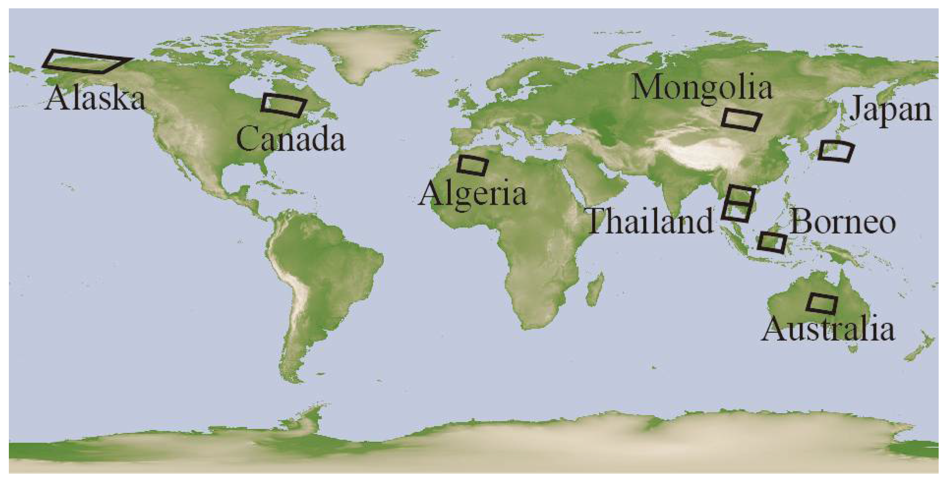
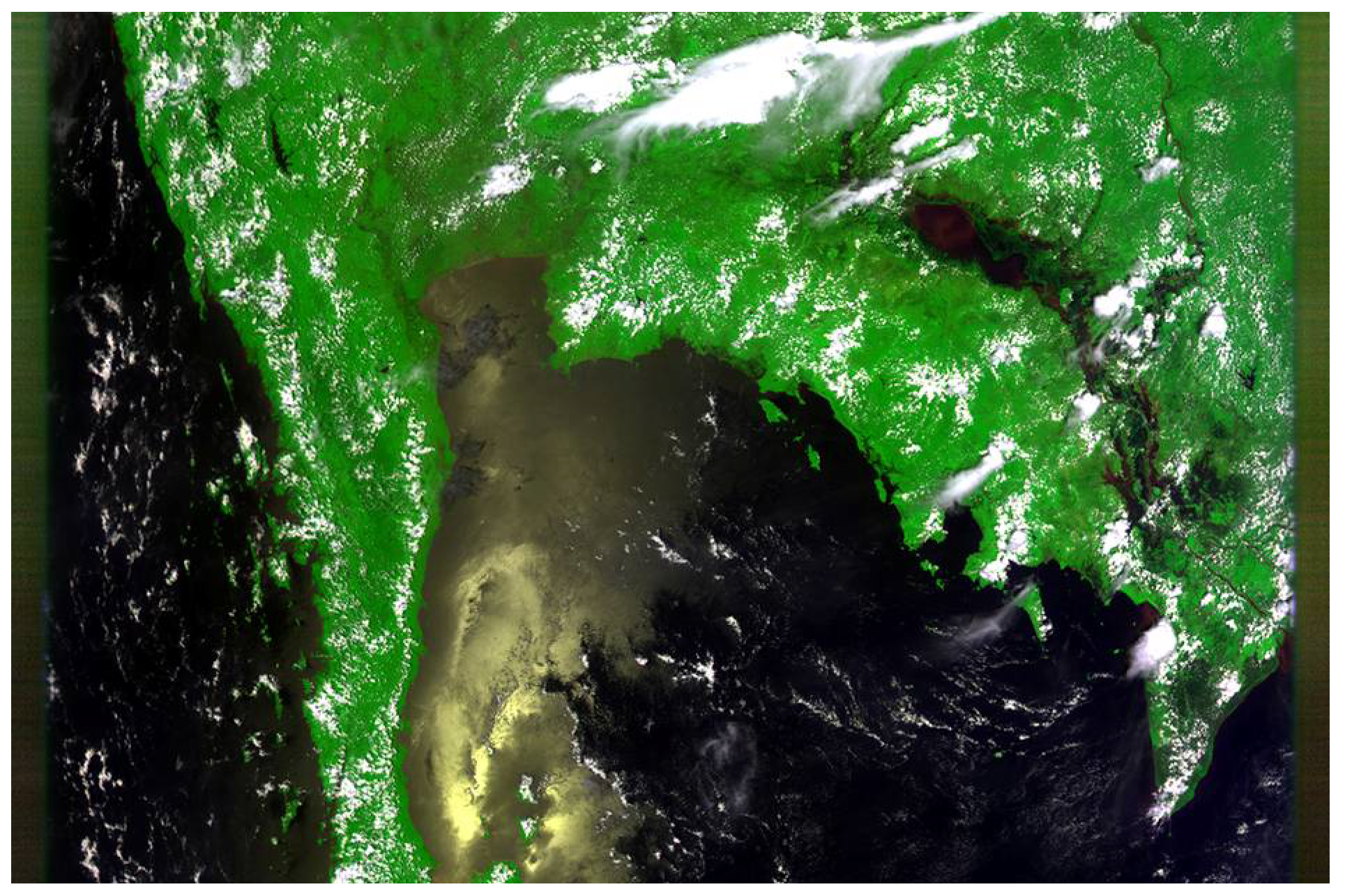
2.1. Satellite Data

We used GOSAT CAI Level 1B products, which can be downloaded from GOSAT Data Archive Service (GDAS, https://data2.gosat.nies.go.jp/index_en.html). GOSAT returns to a similar footprint after 44 orbits (44 CAI paths) in 3 days. The satellite ground path of one orbit is divided into 60 equidistant CAI frames. The study area and data period were the same as those used in a previous study [5] (Figure 1;

Table 1. GOSAT CAI Level 1B product used in this study. Land cover was derived from the MODerate resolution Imaging Spectroradiometer (MODIS) land cover type product (MCD12). Japan scenes include urban areas.

Location (CAI Path_Frame)	Data Period	Land Cover
Australia (4_35)	3 April 2012–3 March 2014	Open shrublands
Japan (5_25)	1 April 2012–1 March 2014	Mixed forests
Borneo (7_31)	3 April 2012–3 March 2014	Evergreen broadleaf forest
Thailand 1 (9_28)	2 April 2012–2 March 2014	Cropland/natural vegetation
Thailand 2 (9_29)	2 April 2012–2 March 2014	Cropland/natural vegetation
Mongolia (10_23)	3 April 2012–3 March 2014	Grasslands
Algeria (22_26)	3 April 2012–3 March 2014	Barren or sparsely vegetated
Canada (32_22)	1 April 2012–1 March 2014	Evergreen needleleaf forest
Alaska (43_19)	1 April 2012–1 March 2014	Open shrublands

). The spatial resolution of these products (pixel size at the nadir) was 500 m and the image size was 2048 × 1355 pixels (approximately 1000 × 680 km) (

Table 2. Specifications of Greenhouse gases Observing SATellite (GOSAT) CAI and GOSAT-2 CAI-2.

Specifications of CAI
Band		Central Wavelength (nm)	Spatial Resolution (m)	Swath (km)
1		380	500	1000
2		674
3		870
4		1600	1500	750
Specifications of CAI-2
Band	Central Wavelength (nm)	Spatial Resolution (m)	View Angle (deg.)	Swath (km)
1	343	460	+20 (Forward)	920
2	443
3	674
4	869
5	1630	920
6	380	460	−20 (Backward)
7	550
8	674
9	869
10	1630	920

).

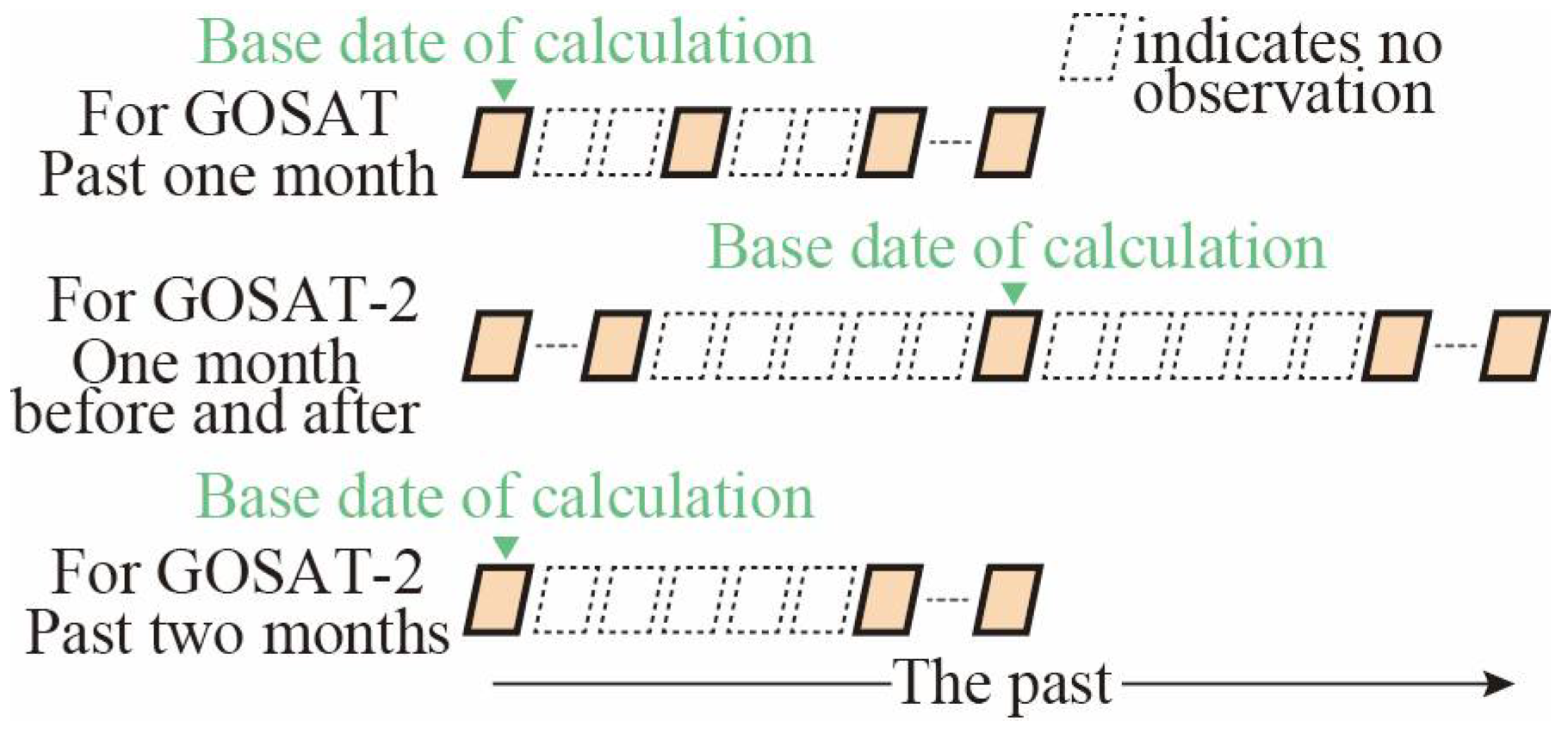
2.2. Methods to Choose the 10 Observations

In this section, we describe three different methods to choose the 10 observations.

Although R_min is created from the CAI L1B data for the past 30 days in GOSAT, with a revisit time of 3 days, R_min for GOSAT-2 is calculated using data obtained over 60 days with a recurrent cycle of 6 days. We compared CLAUDIA1 results obtained using three different methods to choose the 10 observations, i.e., the past one month for GOSAT (−1 month), one month before and after for GOSAT-2 (±1 month), and past two months for GOSAT-2 (−2 months) (Figure 2). The generation procedure for these comparisons is referred to as Procedure 1.

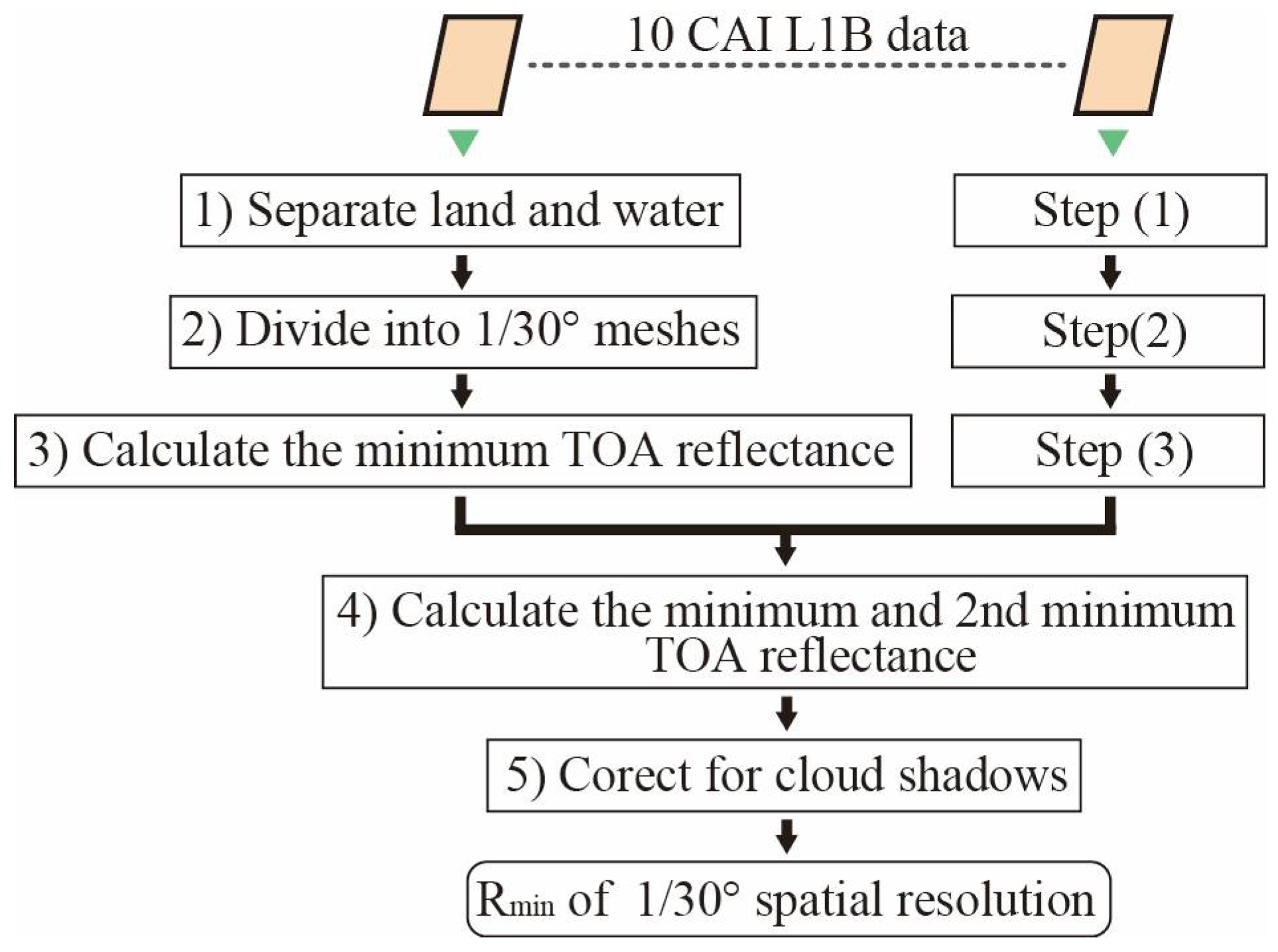
2.3. R_min Generation Procedure for Cloud and Aerosol Imager

In this section, we describe the R_min generation procedures.

R_min at a 1/30° resolution (hereafter R_min1) is generated by the following procedure for CAI version 01.00 (Procedure 1) (Figure 3).

First, steps (i)–(iii) are performed for each CAI L1B product.

• Separate land and water regions using land/sea flag in CAI L1B products
  The land/sea flag is generated from the Shuttle Radar Topography Mission’s (SRTM) 15 arc-seconds land/sea mask [15] and U.S. Geological Survey (USGS) Global Land 1-KM Advanced Very High Resolution Radiometer (AVHRR) Project data [16] for areas with latitudes higher than ±60°.
• Divide region into 1/30° meshes.
• Calculate the minimum TOA reflectance for band 2 for every mesh, treating land and water regions as distinct.

Next, steps (iv)–(v) are performed using 10 CAI L1B products for each mesh.

iv.

Calculate the minimum and second-minimum TOA reflectance for each mesh using the results of step (ii)

v.

Correct for cloud shadows by using the minimum and second-minimum TOA reflectance calculated in step (iv). Cloud shadow correction method, as follows:

$$R_{min}=\{\begin{array}{c}{R}_{2\mathrm{nd}} if\left(R_{2\mathrm{nd},band1}-R_{1\mathrm{st},band1}<0.04\right) and \left(R_{2\mathrm{nd},band3}-R_{1\mathrm{st},band3}>0.02\right)\\ R_{1\mathrm{st}} else\end{array},$$

(1)

where R_1st and R_2nd indicate the minimum and second-minimum reflectance, respectively; R_1st,bandn indicates the minimum reflectance of band n [17] Cloud shadow correction is also necessary because cloud shadows remain in R_min causes to misjudge clear-sky pixels as cloud pixels.

The R_min generation procedure for CAI version 02.00 (Procedure 2) differs from Procedure 1 as follows: it includes the addition of a simple cloud screening test; the use of band 1, rather than band 2, to calculate the minimum TOA reflectance; steps (ii)–(iii) are not performed in Procedure 2; and an iterative process for (iv)–(v) is performed. R_min at a 500-m spatial resolution (hereafter, R_min2) was calculated.

2.4. Comparative Analysis

In this section, we describe evaluation indices used in this study.

In this study, “degree of agreement (DA)” was defined as the ratio of the number of pixels for which the standard image and output from the cloud discrimination algorithm agreed to the total number of pixels in the input image. “Overlook” was defined as the ratio of the number of pixels identified as clear-sky in the output and cloudy in the standard image to the number of pixels that were identified as cloudy in the standard image. “Overestimate” was defined as the ratio of the number of pixels identified as cloudy in the output and clear-sky in the standard image to the number of pixels identified as clear-sky in the standard image. Each was defined by the following equations (the std subscript indicates standard results):

$$\mathrm{DA}=\frac{\mathrm{Both}\mathrm{cloudy}+\mathrm{Both}\mathrm{clear}-\mathrm{sky}}{\mathrm{Total}\mathrm{number}\mathrm{of}\mathrm{pixels}},$$

(2)

$$\mathrm{Overlook}=\frac{{\mathrm{Clear}-\mathrm{sky}\mathrm{despite}\mathrm{cloudy}}_{\mathrm{std}}}{{\mathrm{Both}\mathrm{cloudy}+\mathrm{Clear}-\mathrm{sky}\mathrm{despite}\mathrm{cloudy}}_{\mathrm{std}}},$$

(3)

$$\mathrm{Overestimate}=\frac{{\mathrm{Cloudy}\mathrm{despite}\mathrm{clear}-\mathrm{sky}}_{\mathrm{std}}}{{\mathrm{Both}\mathrm{clear}-\mathrm{sky}+\mathrm{Cloudy}\mathrm{despite}\mathrm{clear}-\mathrm{sky}}_{\mathrm{std}}}.$$

(4)

3. Results

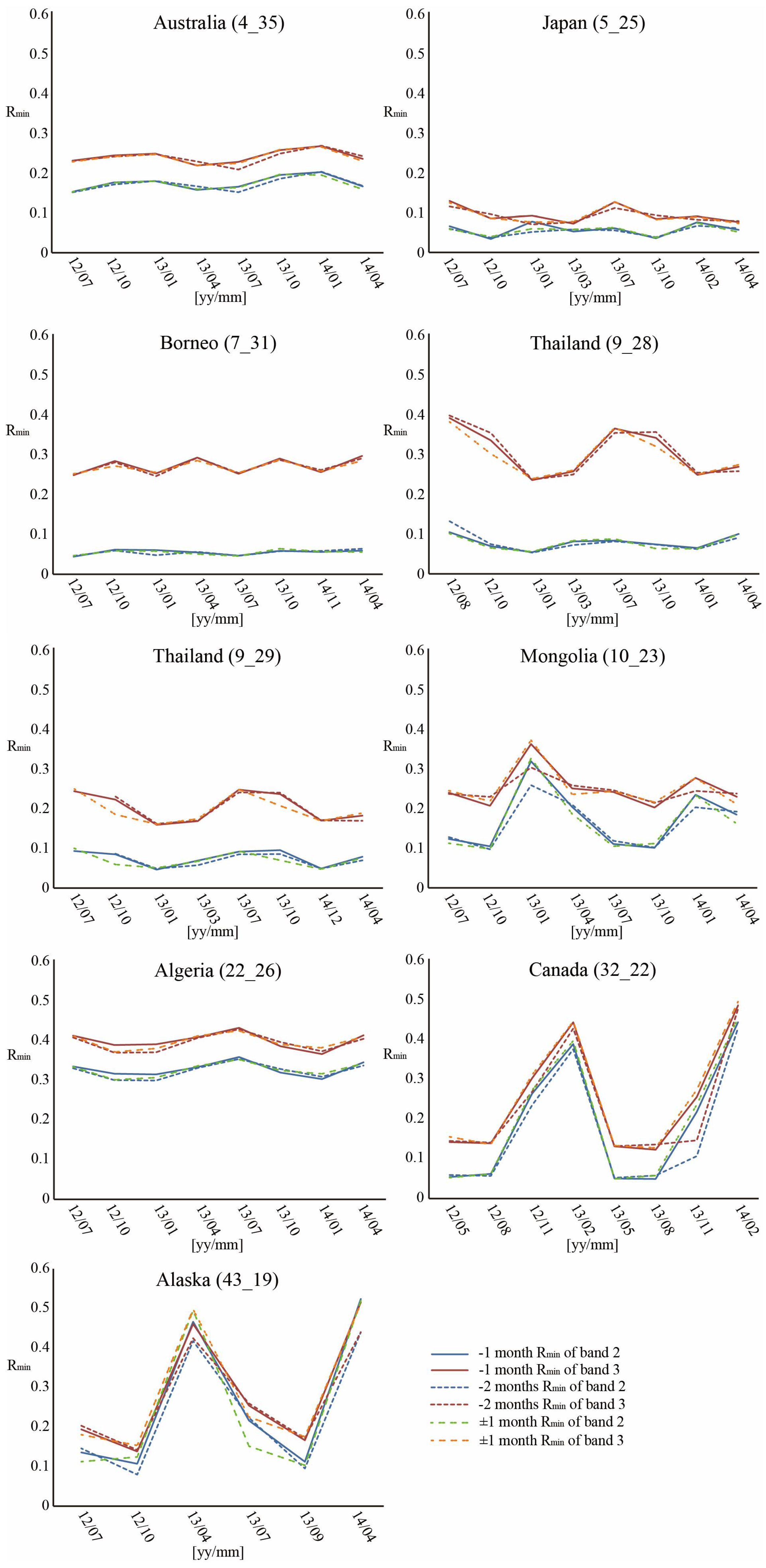
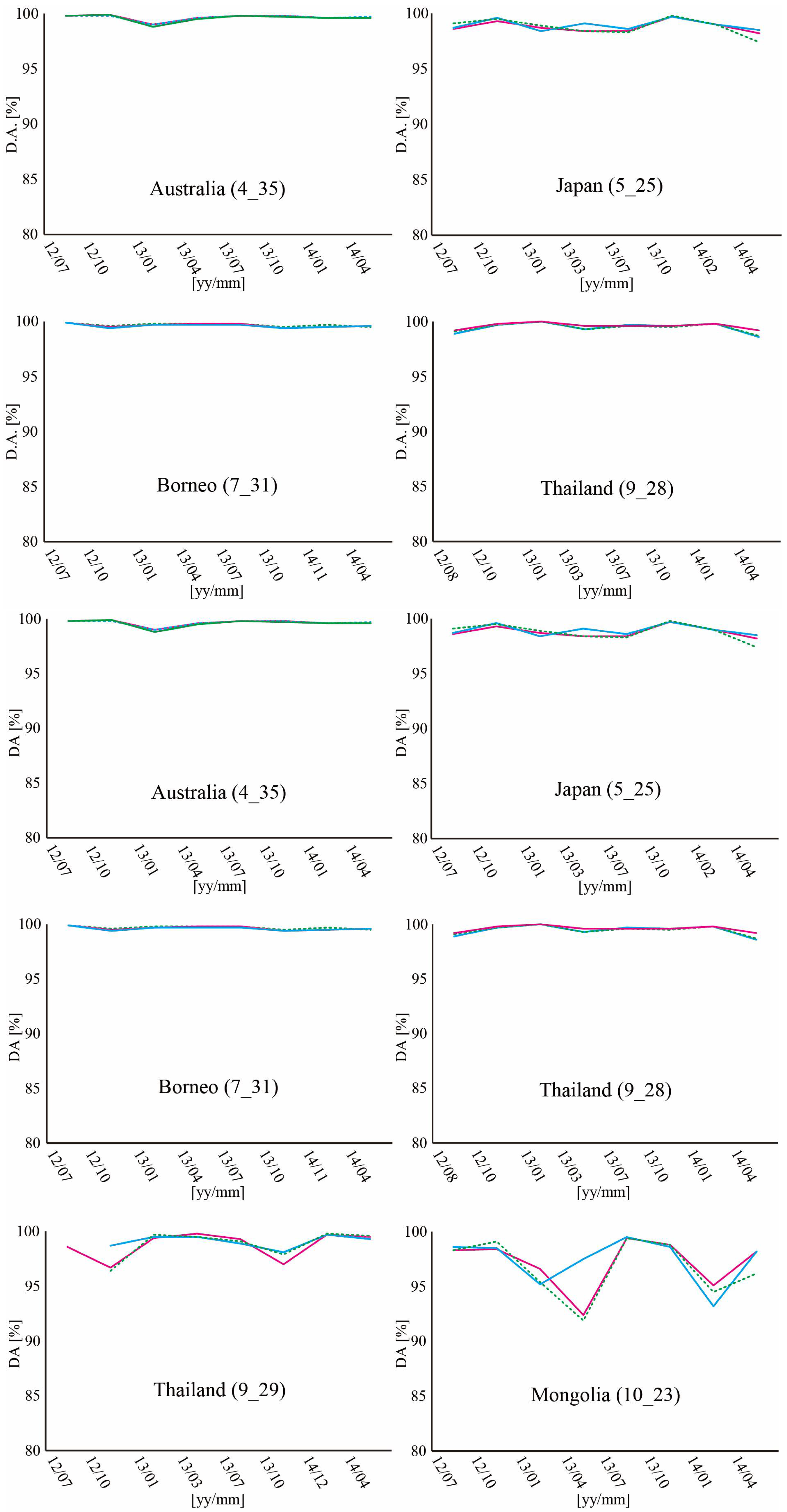
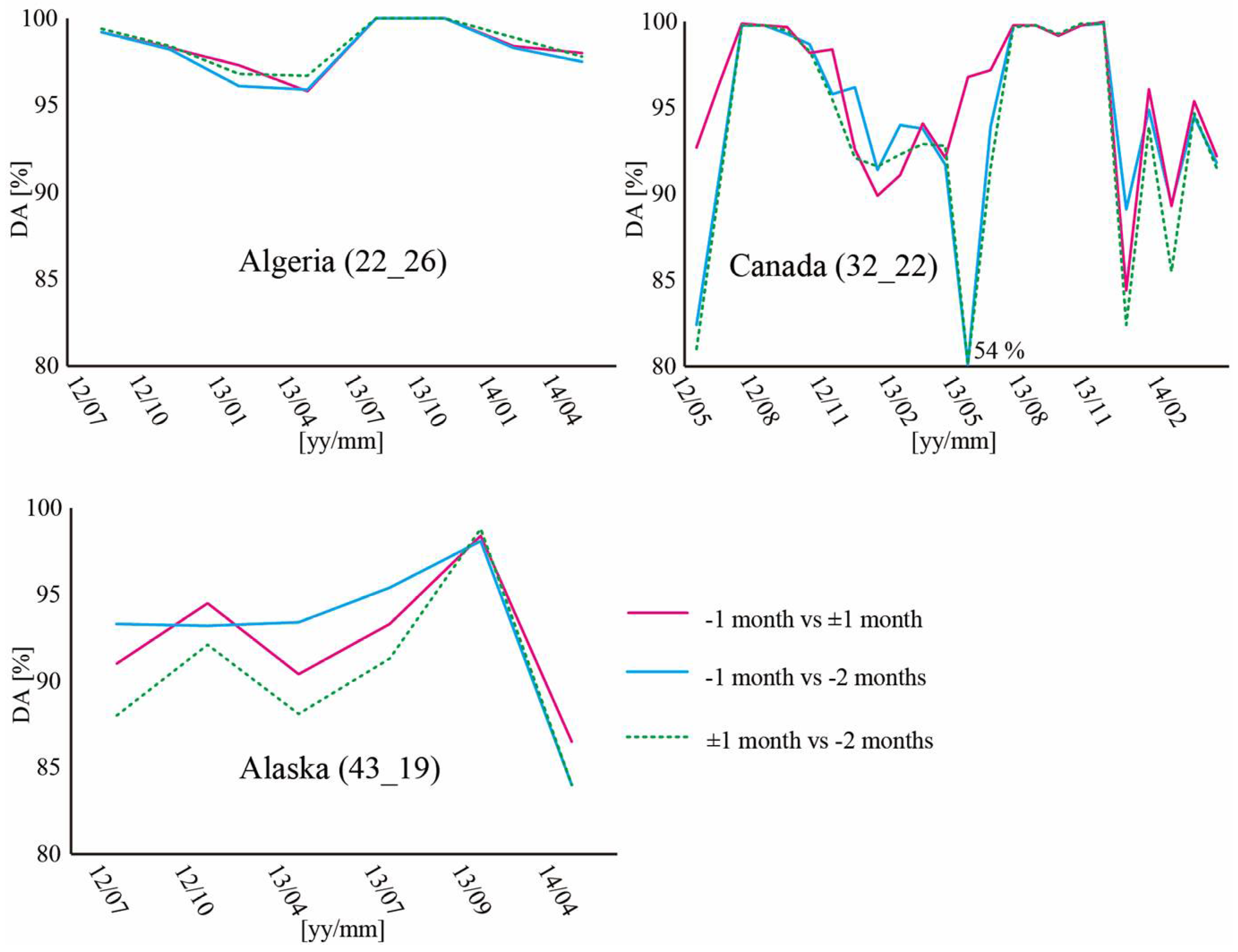
3.1. Comparison among Methods to Choose the 10 Observations

We compared R_min calculated using different methods to choose the 10 observations. Figure 4 shows the averaged R_min for each CAI scene generated using these different methods, i.e., −1 month, −2 months, and ±1 month.

In Australia, Borneo, and Algeria, there were no marked seasonal changes or differences between −1 month R_min, −2 months R_min, and ±1 month R_min. In Japan and Thailand, every R_min for band 3 in the summer for the Northern Hemisphere was greater than those for the other seasons due to seasonal vegetation changes. In Japan, Mongolia, Canada, and Alaska, every R_min for both bands 2 and 3 in the winter for the Northern Hemisphere was greater than those in the other seasons due to snow or ice cover.

Figure 5 shows comparative cloud discrimination results using various methods to choose the 10 observations.

In Australia, Borneo, and Thailand (Path 9, Frame 28), DA between −1 month, ±1 month, and −2 months was always greater than 99%, suggesting that there was no difference between methods. In Japan, there was a slight difference (the lowest DA was 97.4%) in cloud discrimination results among methods. In Algeria, there was a difference (the lowest DA was 95.8%) in cloud discrimination results. In Thailand (Path 9, Frame 29), there was a difference in cloud discrimination results in October (the lowest DA was 96.4%). In Mongolia, Canada, and Alaska, there was a difference (the lowest DA was 54.3%) among R_min methods with snow or ice.

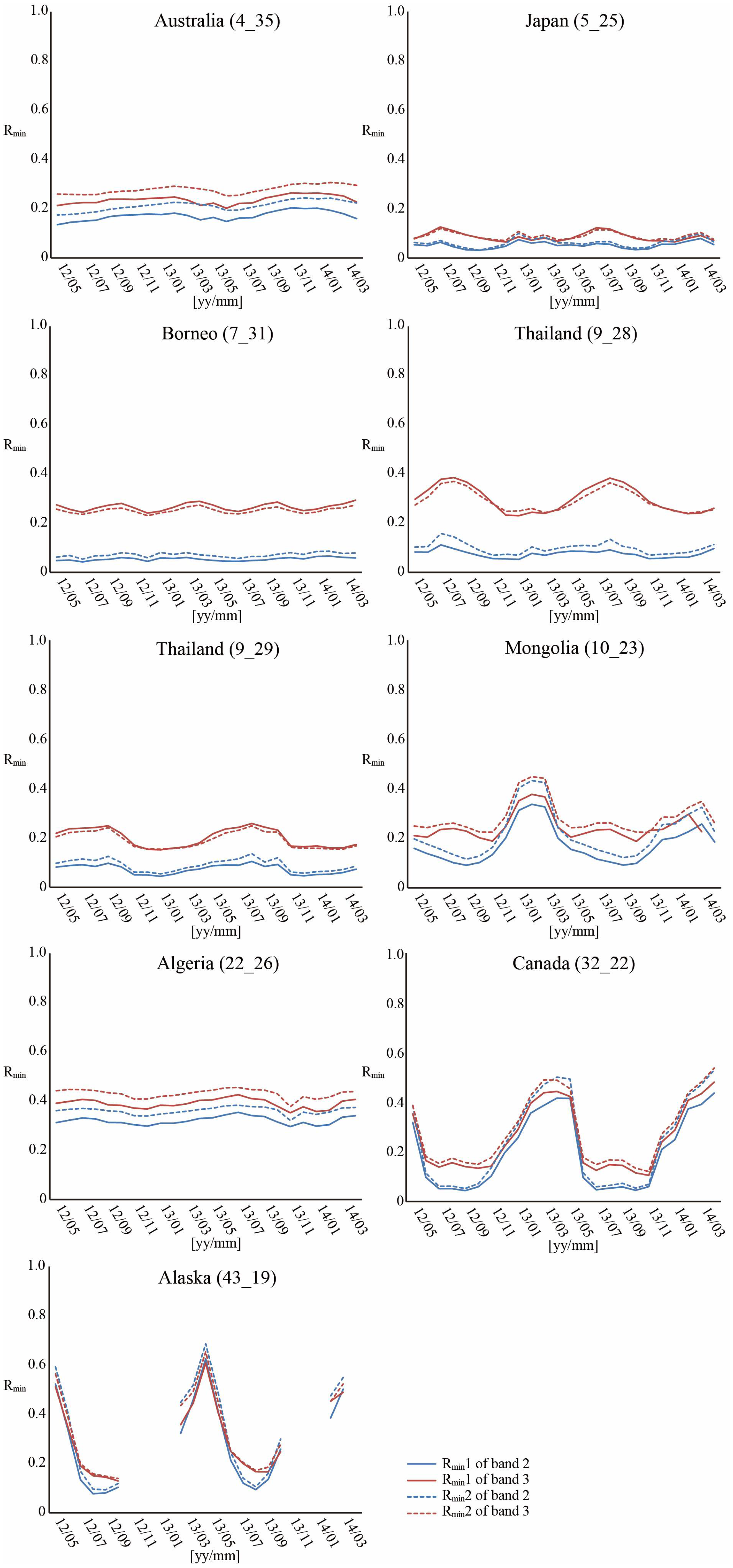
3.2. Comparison among Different Generation Procedures

We compared R_min calculated using different generation procedures. Figure 6 shows the averaged R_min in each CAI scene for various land cover types.

R_min1 of band 2 was lower than R_min2 of band 2 because the minimum TOA reflectance in 1/30° meshes was calculated using band 2 in Procedure 1 and the minimum TOA reflectance in each pixel was calculated in Procedure 2.

R_min1 of band 3 was greater than R_min2 of band 3 in Japan, Borneo, and Thailand. In Japan, Mongolia, Canada, and Alaska, both bands 2 and 3 in the winter for the Northern Hemisphere were greater than those in other seasons due to snow or ice cover.

In Figure 7, for Overlook and Overestimate, cloud discrimination results using R_min1 were used as standard images. Overlook was greater than Overestimate, except in Canada. This means that R_min2 tends to identify clear-sky more frequently than R_min1. This can be explained by the following reasons.

• R_min1 of band 2 is lower than R_min2 of band 2.
• R_min of band 2 is used for cloud discrimination on land regions. Land pixels occupy most of the test scenes.

There were also water pixels and some complex effects, such as cloud remains in R_min, the difference between bands used to generate R_min, and a simple cloud screening test of Procedure 2 (Figure 8).

In Australia and Algeria, which have highly reflective surfaces, Overlook was always high (average Overlook was 36.4%), regardless of the season. DA in Alaska was lower than that in the other regions. In Japan, Mongolia and Canada, Overlook in the winter for the Northern Hemisphere was greater than that in the other seasons, so that DA in winter was lower than that in the other seasons.

4. Discussion

4.1. Differences among Methods Used to Choose the 10 Observations

First, we discuss the differences in R_min with respect to the method used to obtain the 10 observations (Figure 4). In Thailand, ±1 month R_min was lower than −1 month R_min and −2 months R_min in October. This may explain why R_min in November was lower than that in summer in the Northern Hemisphere. In other words, ±1 month R_min preempts the R_min decline due to seasonal vegetation changes. In the same way, ±1 months R_min preempts the thawing of snow in Alaska in July. Conversely, −2 months R_min was lower than −1 month R_min and ±1 month R_min in Mongolia in January and in Canada in November. This means that −2 months R_min included data for areas before any snowfall.

Second, we discuss cloud discrimination using R_min obtained by different methods for choosing the 10 observations (Figure 5). In Japan, there was a slight difference in cloud discrimination results that could be explained by overlooked optically thin clouds in each result. This was explained by the use of R_min for cloud remains over the ocean (Figure 9).

In Algeria, there was a difference in cloud discrimination results due to the overestimation of clouds (Figure 5) arising from the use of R_min values when cloud shadow is present (Figure 10).

In Thailand (Path 9, Frame 29), there was a difference in cloud discrimination results in October (Figure 5). The −2 months R_min was generated from CAI data from the beginning of August to the beginning of October, −1 month R_min was generated from CAI L1B data from the beginning of September to the beginning of October, and ±1 month R_min was generated from CAI L1B data from the beginning of September to late October. There were sun-glint regions over the ocean until the beginning of October in this area (Figure 11). Cloud discrimination results overlook optically thin clouds when R_min was generated from only the sun-glint period.

In Mongolia, Canada, and Alaska, there was a difference in R_min depending on snow or ice (Figure 5). In particular, there was a difference between R_min generated from CAI data during only the snow-covered period and R_min generated from CAI data including the period after snow melting. The former had a tendency to overlook clouds, and the latter had a tendency to misjudge snow and ice as clouds.

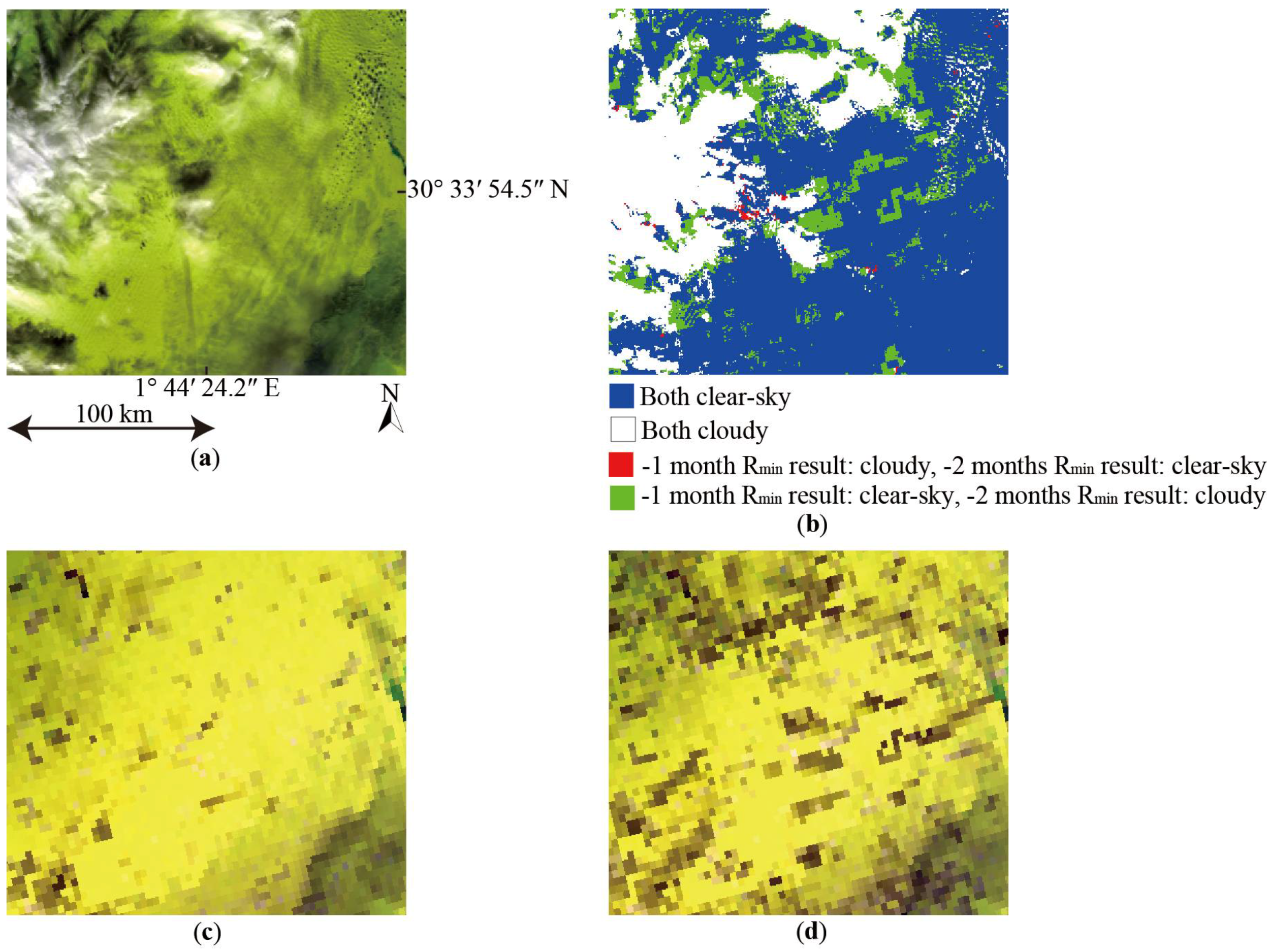
4.2. Discussion of the Differences of R_min among Generation Procedures

In this section, we evaluated differences in R_min depending on the generation procedure (Figure 6).

R_min1 of band 3 was greater than R_min2 of band 3 in Japan, Borneo, and Thailand. Vegetation has a low reflectance in the visible red band and high reflectance in the NIR band. Thus, estimates of R_min using band 2 have a tendency to select vegetation pixels. Accordingly, R_min1 of band 3 was greater than R_min2 of band 3 in regions with high vegetation cover. In Japan and Thailand, R_min for band 3 from spring to autumn in the Northern hemisphere was greater than that in the other seasons due to seasonal vegetation changes.

Neither R_min1 nor R_min2 could remove clouds in regions with a high cloud cover ratio or cloud shadows on regions with high surface reflectance. In general, tropical rainforests have a high cloud cover ratio due to evaporation along with photosynthesis of vegetation. As shown in Figure 12a,b, many clouds remain in both R_min1 and R_min2, although R_min1 was smoothed somewhat owing to its lower spatial resolution than that of R_min2. For desert regions, there were whitish pixels for which R_min of band 1 was greater than that around pixels in a RGB composite image of R_min1 (Figure 12d). The R_min generation procedure using band 2 could not remove optically thin clouds in highly reflective regions. Furthermore, both R_min1 and R_min2 could not remove cloud shadows in highly reflective regions (Figure 12d,e).

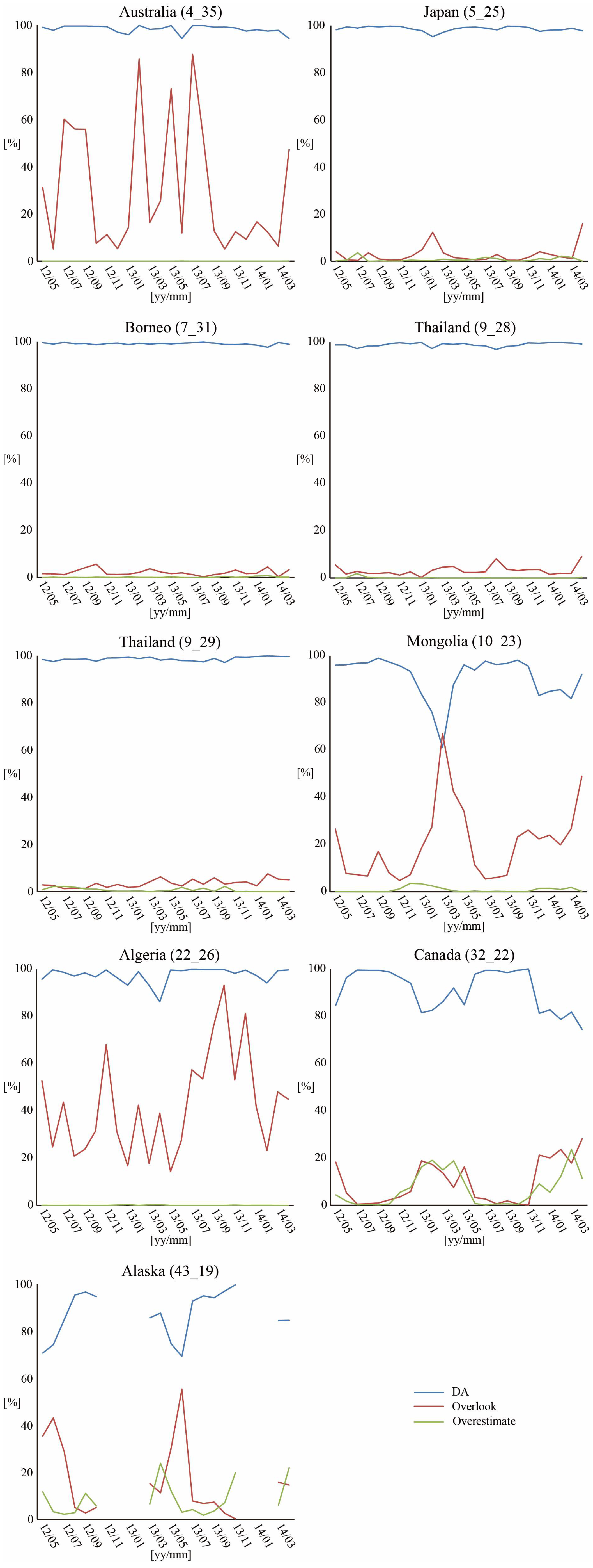
4.3. Discussion of the Differences of Cloud Discrimination Results among Generation Procedures

In this section, we evaluated cloud discrimination using R_min obtained by different generation procedures (Figure 7).

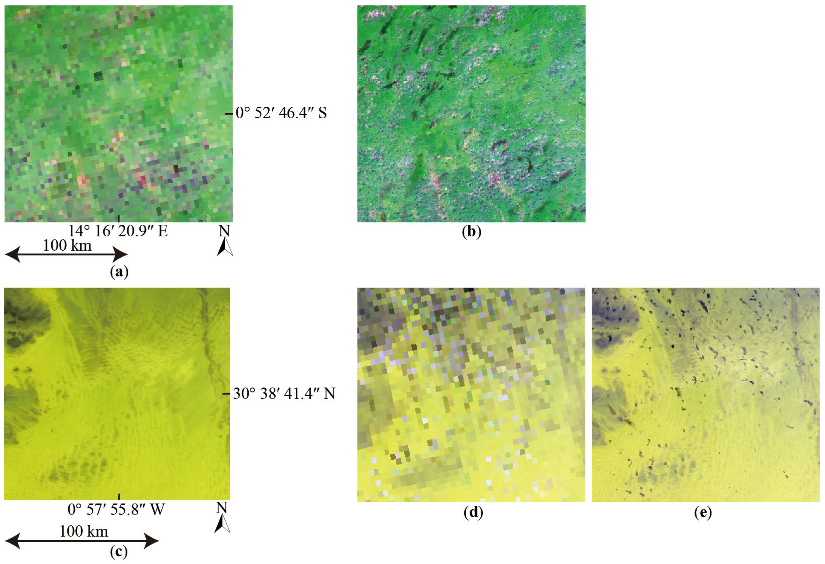
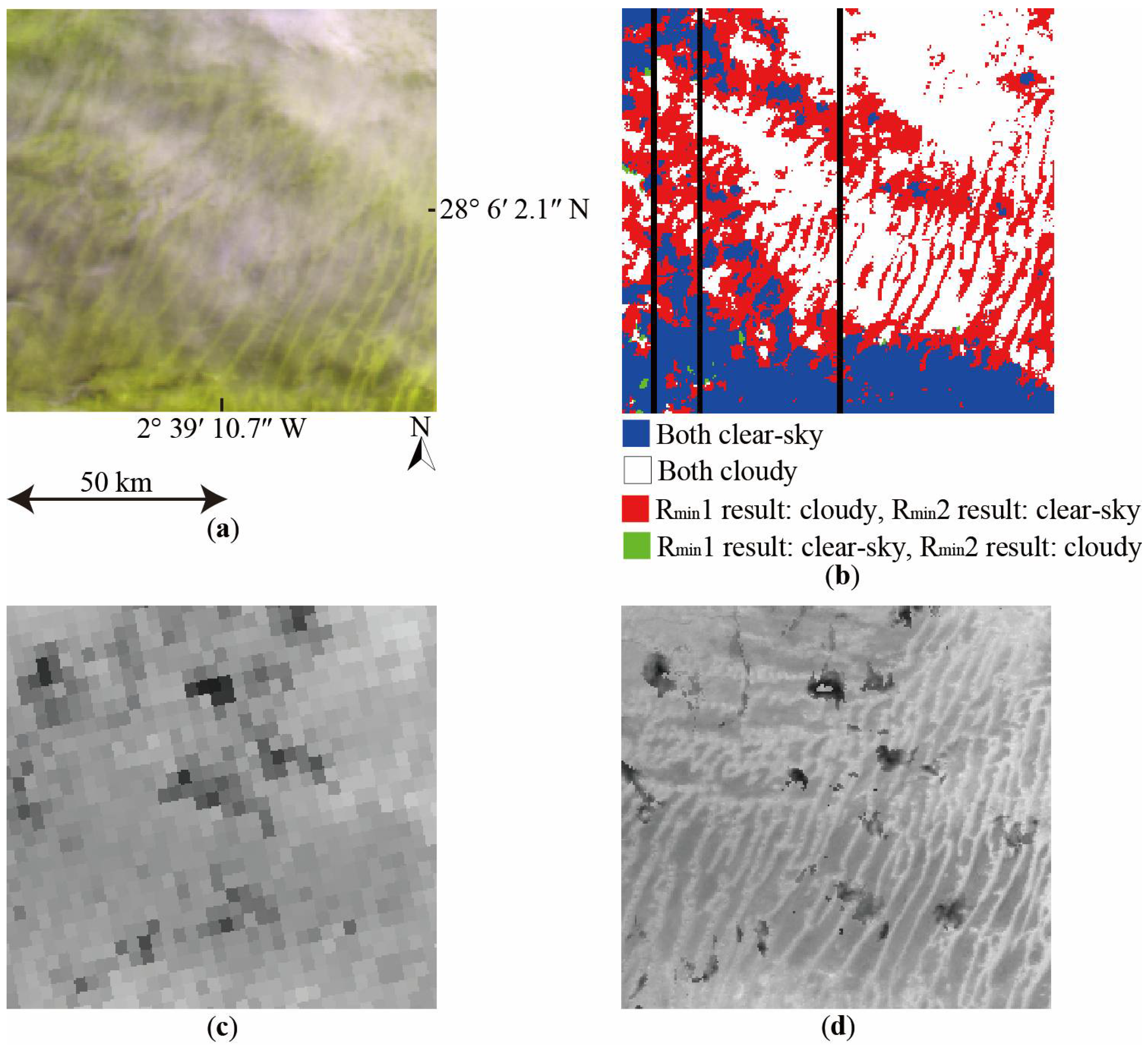
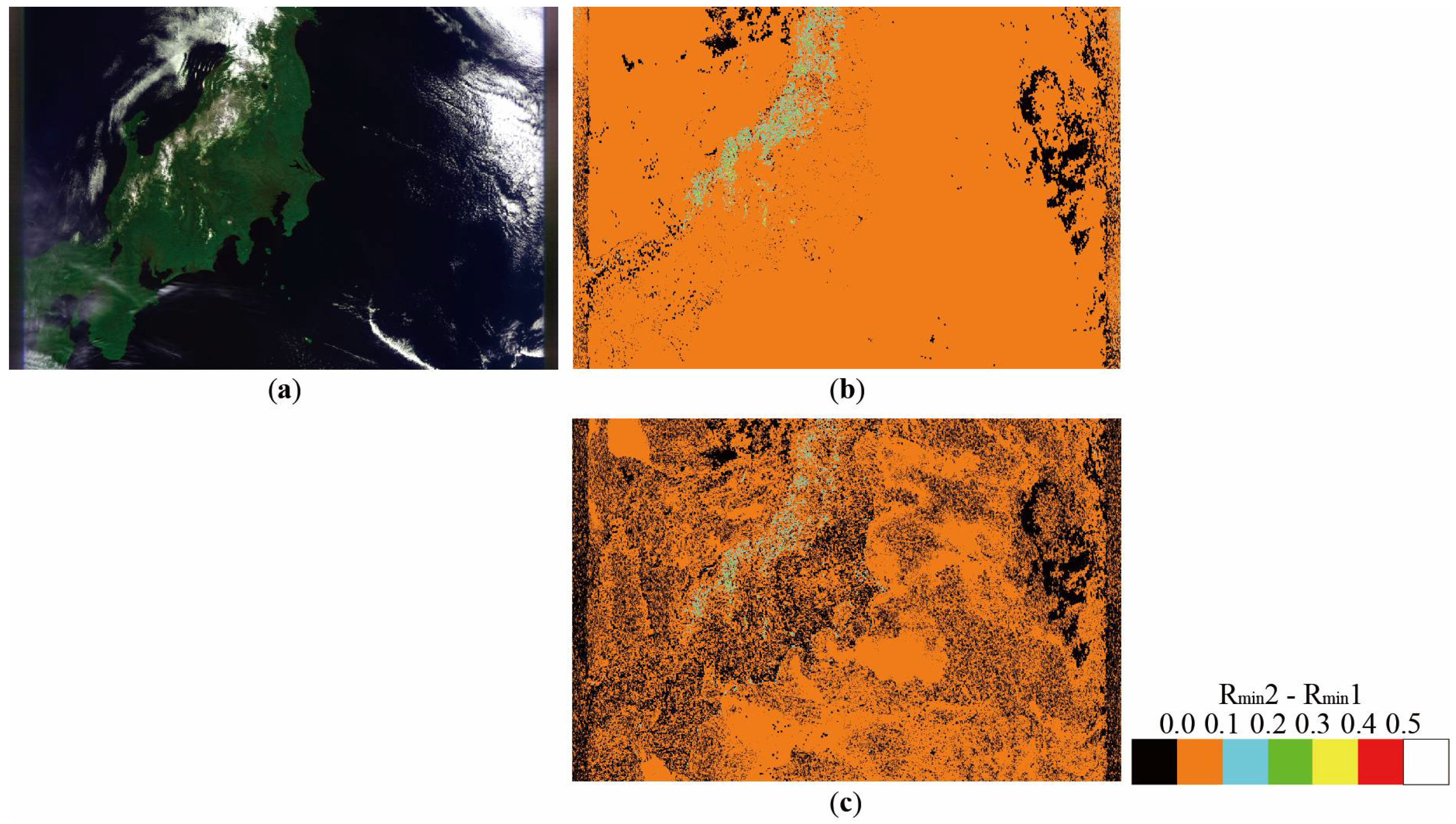
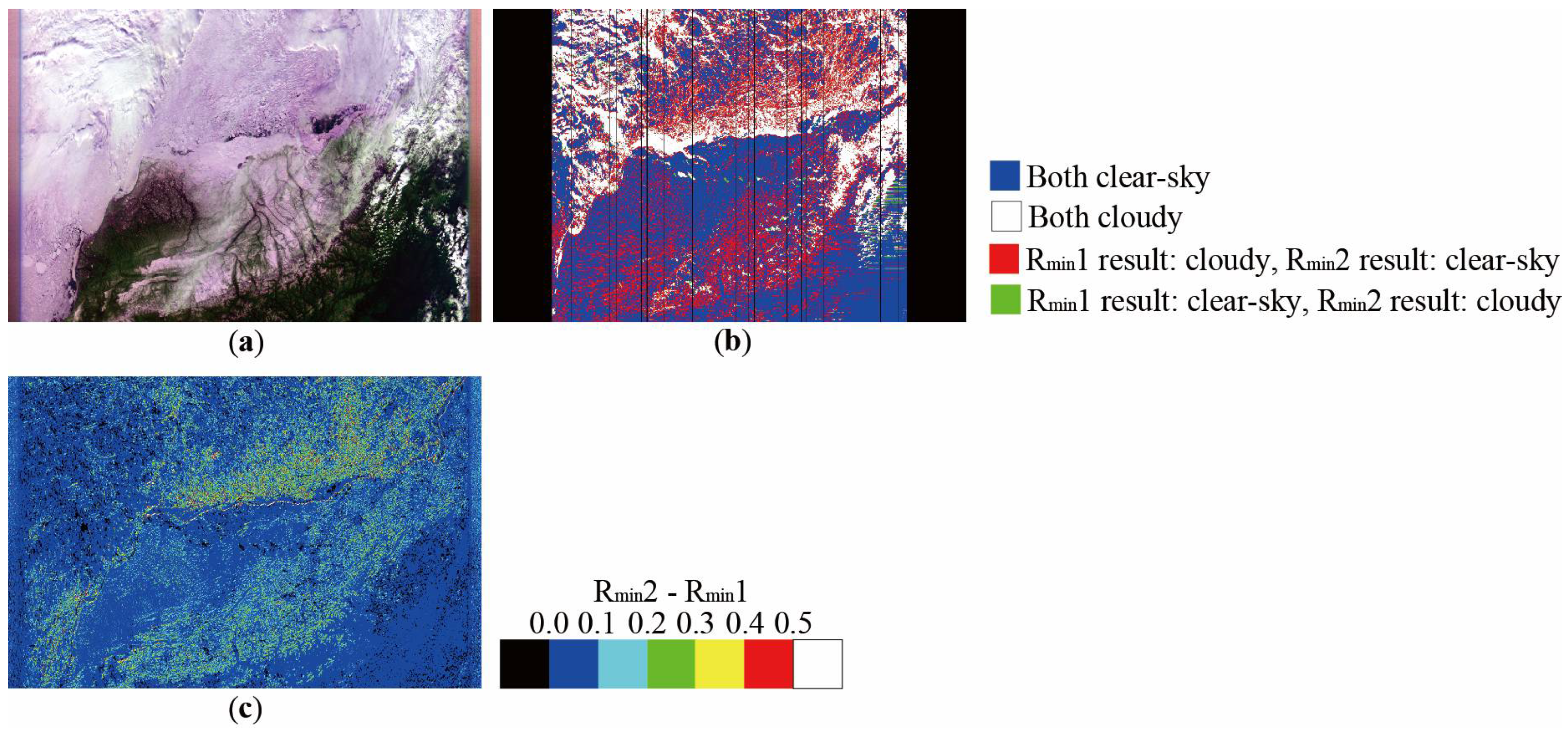
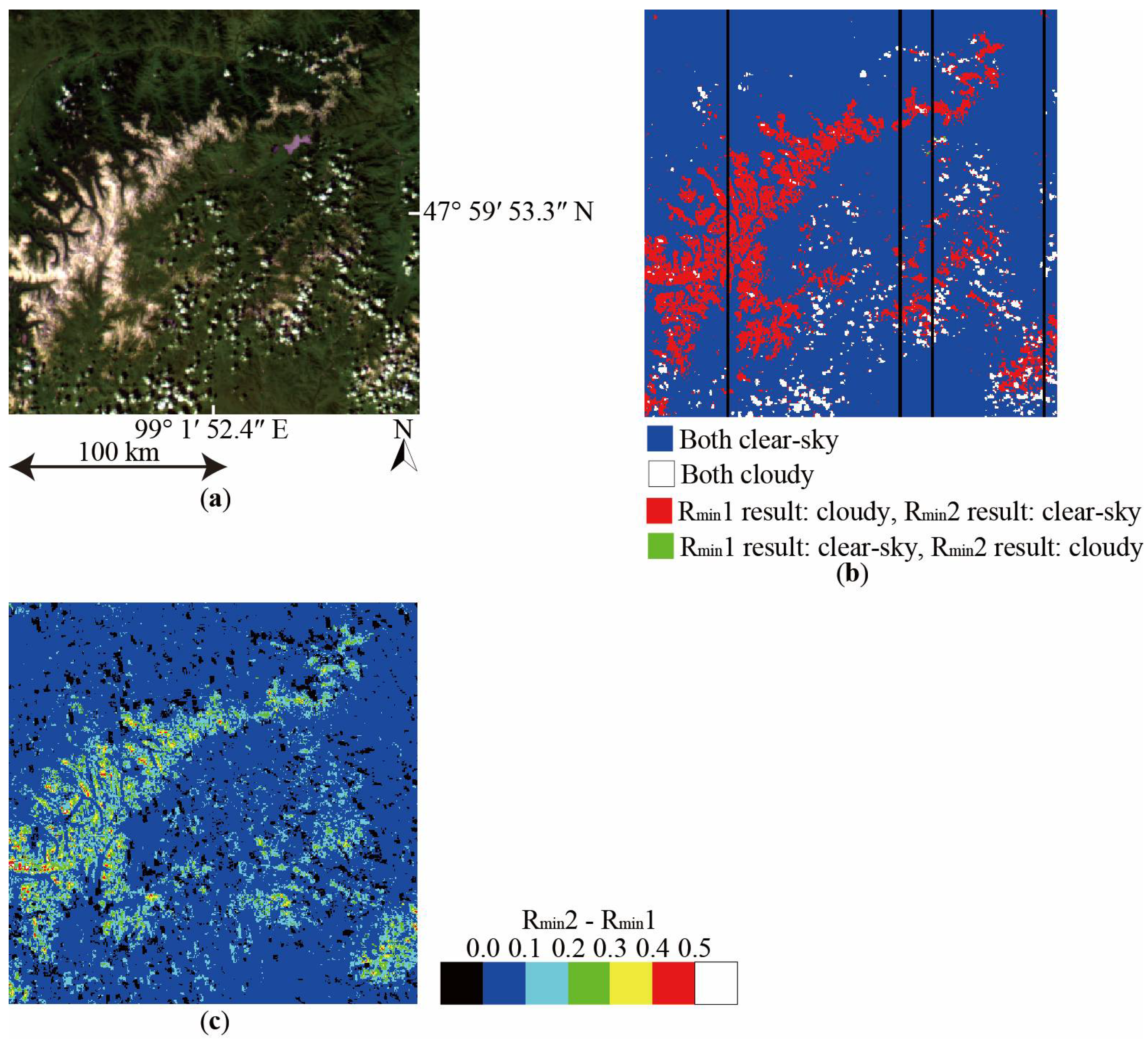
4.3.1. Highly Reflective Surface

In Australia and Algeria, which have highly reflective surfaces, Overlook was always high, regardless of the season. R_min2 results had a tendency to overlook optically thin clouds in comparison with R_min1 results (Figure 13). On the other hand, the local highly reflective surface where R_min1 incorrectly identified clouds was slightly improved in the R_min2 results (Figure 14). Procedure 1 chooses lower TOA reflectance pixels in 1/30° meshes when there is a local highly reflective surface. For this reason, R_min2 results have a tendency to overlook optically thin clouds and R_min1 results have a tendency to overestimate local high reflectance surfaces as clouds in regions with highly reflective surfaces. However, there are few cases in which cloud shadows cause the misidentification of highly reflective surfaces as cloudy.

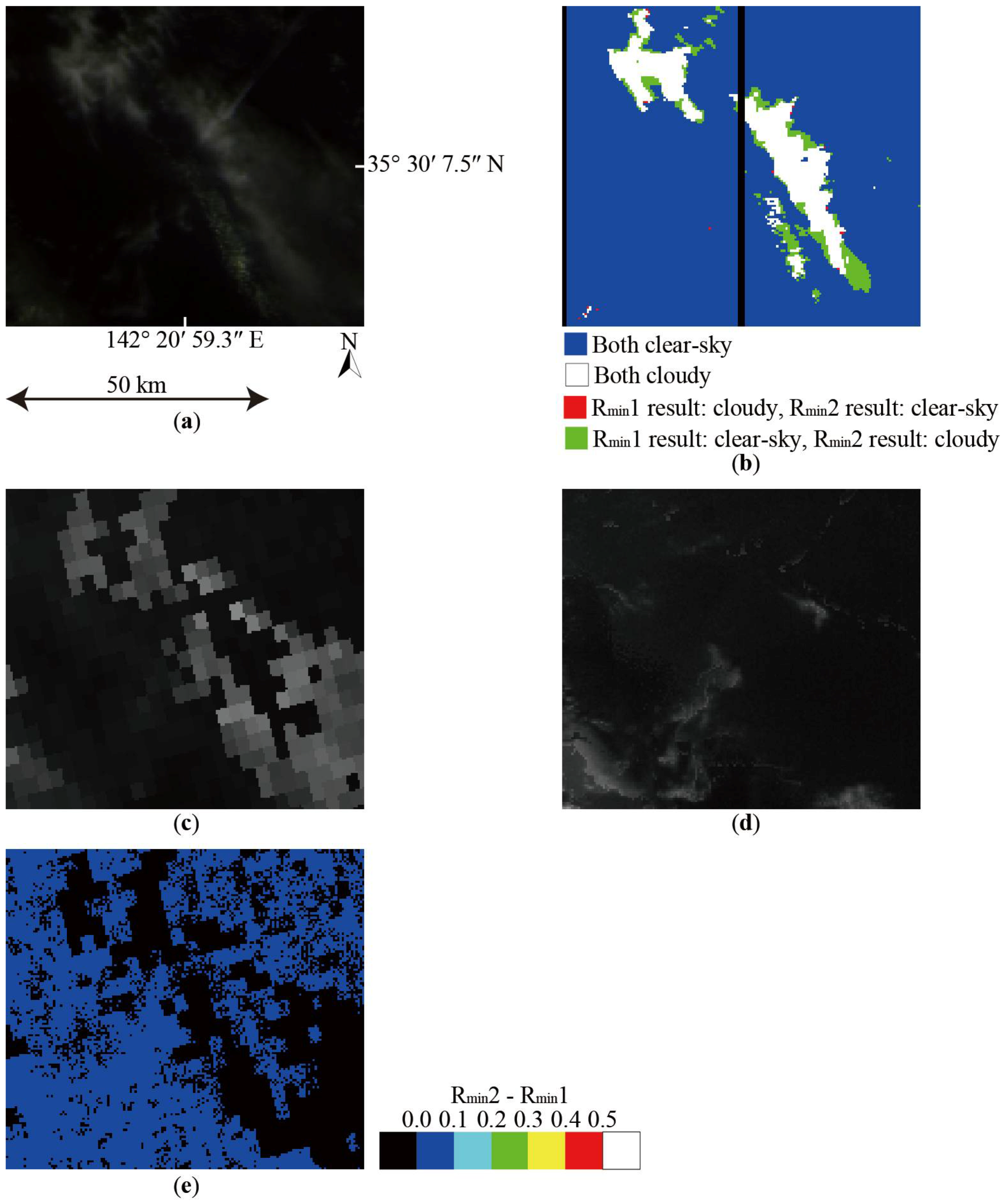
4.3.2. Snow or Ice

In Japan, Mongolia, and Canada, DA in winter of the Northern Hemisphere was lower than that in the other seasons (Figure 7). Since the CAI is not equipped with thermal infrared bands, cloud discrimination based on the temperature at the top of clouds is not feasible. Accordingly, it is difficult to discriminate between clouds and ice or snow [5]. The lower DA in Alaska than that in the other regions (Figure 7) can be attributed to the same source of error. However, regions with ice and snow, where R_min1 results were misidentified as clouds, were slightly improved in R_min2 (Figure 15). This can be explained by the tendency for R_min1 to be lower than R_min2, and cases in which R_min1 chooses pixels lacking snow around snow pixels in 1/30° meshes (Figure 16).

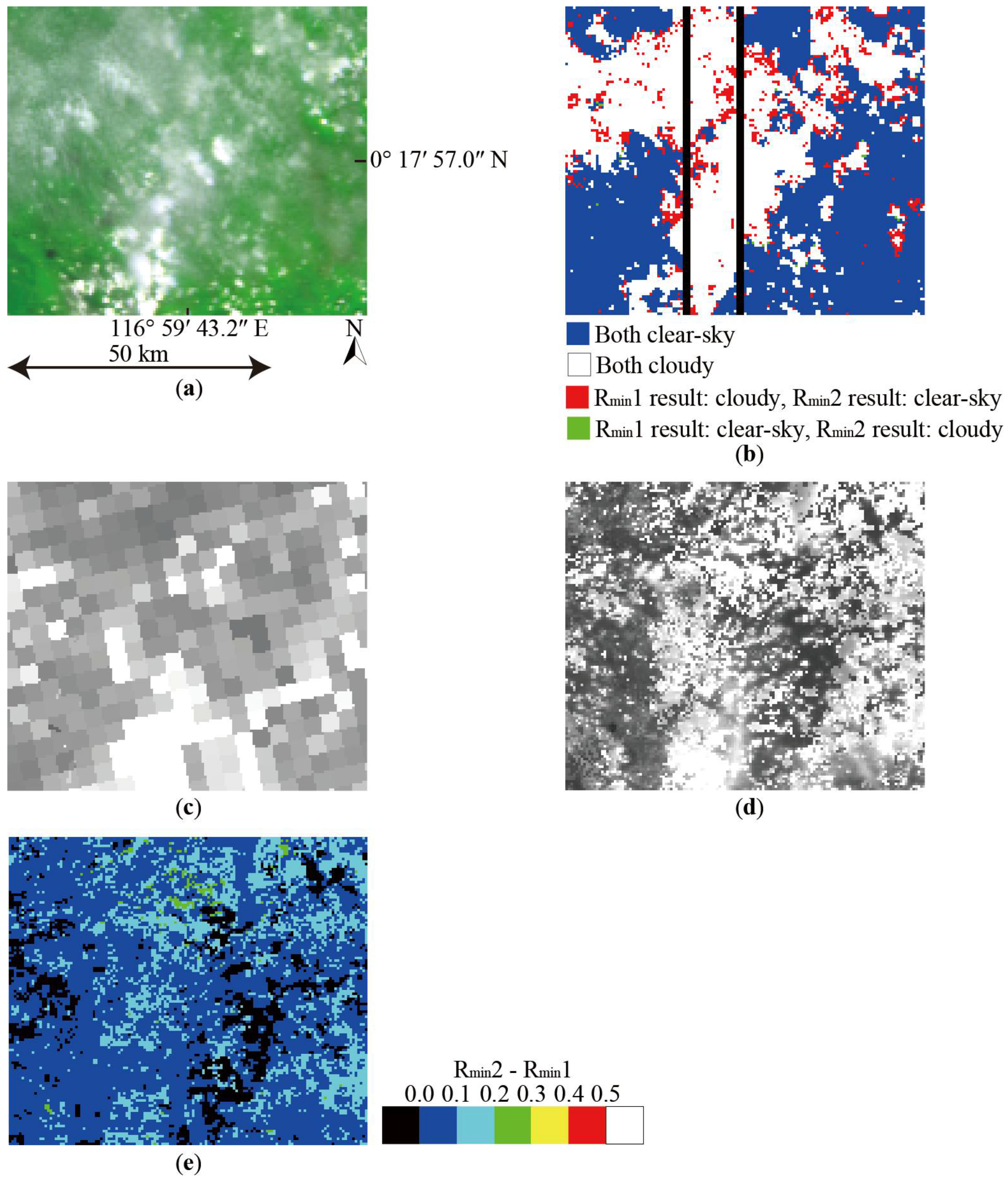
4.3.3. Cloud Remain

In some cases, R_min2 was lower than R_min1 according to cloud remains in R_min due to the high cloud cover ratio, which caused Overestimate (Figure 17). Overestimates in Canada and Alaska were greater than those in the other regions (Figure 7). Canada and Alaska, there was abundant snow or ice; accordingly, there were not almost areas that were judged as clear-sky areas in the R_min1 results. Therefore, when few clear-sky pixels in the R_min1 results changed to cloudy pixels in the R_min2 results, Overestimate was greater, according to the definition.

In Borneo and Thailand, in some cases, R_min2 results overlooked optically thin clouds, even though R_min1 results could identify the clouds over land regions, according to cloud remains in R_min, due to a high cloud cover ratio (Figure 18). These cases on low reflectance surface were opposite from cases with highly reflective surfaces shown in Figure 17.

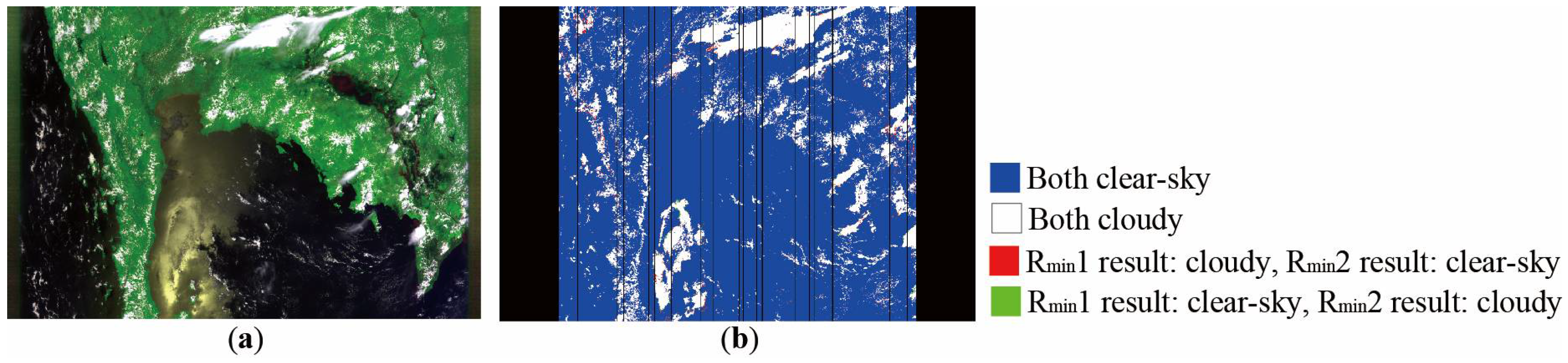
4.3.4. The Boundaries between Land and Water

There were unexpected R_min1 results in which clear-sky pixels were misidentified as clouds over water regions near the boundaries between land and water; however, R_min2 results could identify these areas as clear sky (Figure 19). Procedure 1 chooses surrounding water pixels because its spatial resolution is 1/30° when there are mixed pixels of land and water.

4.3.5. Sun-Glint

There were not almost differences between R_min1 results and R_min2 results in water sun-glint regions (Figure 20).

5. Conclusions

In this study, we had two major goals:

• To compare R_min calculated using different methods to choose 10 observations.
• To compare R_min using different generation procedures and spatial resolutions.

The method used to choose the 10 observations had a minor impact on cloud discrimination results, with some exceptions, such as snow-covered regions and sun-glint regions. In Japan, the difference was caused by using R_min when clouds over the ocean were not removed. However, this difference is not explained by differences in the selection of the 10 observations, but by random variation. In the same manner, the difference caused by using R_min in which cloud shadows were not removed in Algeria does not depend on the way in which the 10 observations were chosen. R_min for GOSAT-2 (−2 months and ±1 month) had a higher potential for the 10 observations to include the non-sun-glint period in sun-glint regions than R_min for GOSAT (−1 month), because the data period used to generate R_min for GOSAT-2 was longer than that for GOSAT. This has the effect of reducing the overlook of clouds. CLAUDIA raises thresholds in water sun-glint regions under the assumption that R_min does not include water sun-glint pixels. Furthermore, R_min for GOSAT-2 (−2 months and ±1 month) has a higher potential to use 10 observations that include the period after snow melting in snow-covered regions than R_min for GOSAT (−1 month). GOSAT-2 had fewer cases in which clouds were overlooked, but more cases in which snow or ice was misjudged as clouds compared with GOSAT in snow-covered regions. With respect to R_min of −2 months or ±1 month for GOSAT-2, R_min of ±1 months was better than that of −2 months in general because the average for ±1 month agreed with observations. From the viewpoint of steady processing for GOSAT-2 CAI-2 data, cloud discrimination processing using R_min of ±1 month cannot be performed unless a period of 1 month from the observation date elapses.

This study also demonstrated the impact of using R_min generated by different procedures. Cloud discrimination results using R_min2 generated by Procedure 2 had the following tendencies in comparison with results using R_min1 generated by Procedure 1.

• R_min2 results had a greater tendency to identify clear sky in comparison with R_min1 results.
• R_min2 results had a tendency to overlook optically thin clouds over local highly reflective surfaces.
• R_min2 results had a tendency to accurately identify local highly reflective surfaces as clouds.
• Ice and snow regions where R_min1 results misidentified clouds were slightly improved in R_min2 results.
• For regions with a high cloud cover ratio, R_min2 results occasionally overlooked optically thin clouds according to cloud remains in R_min.
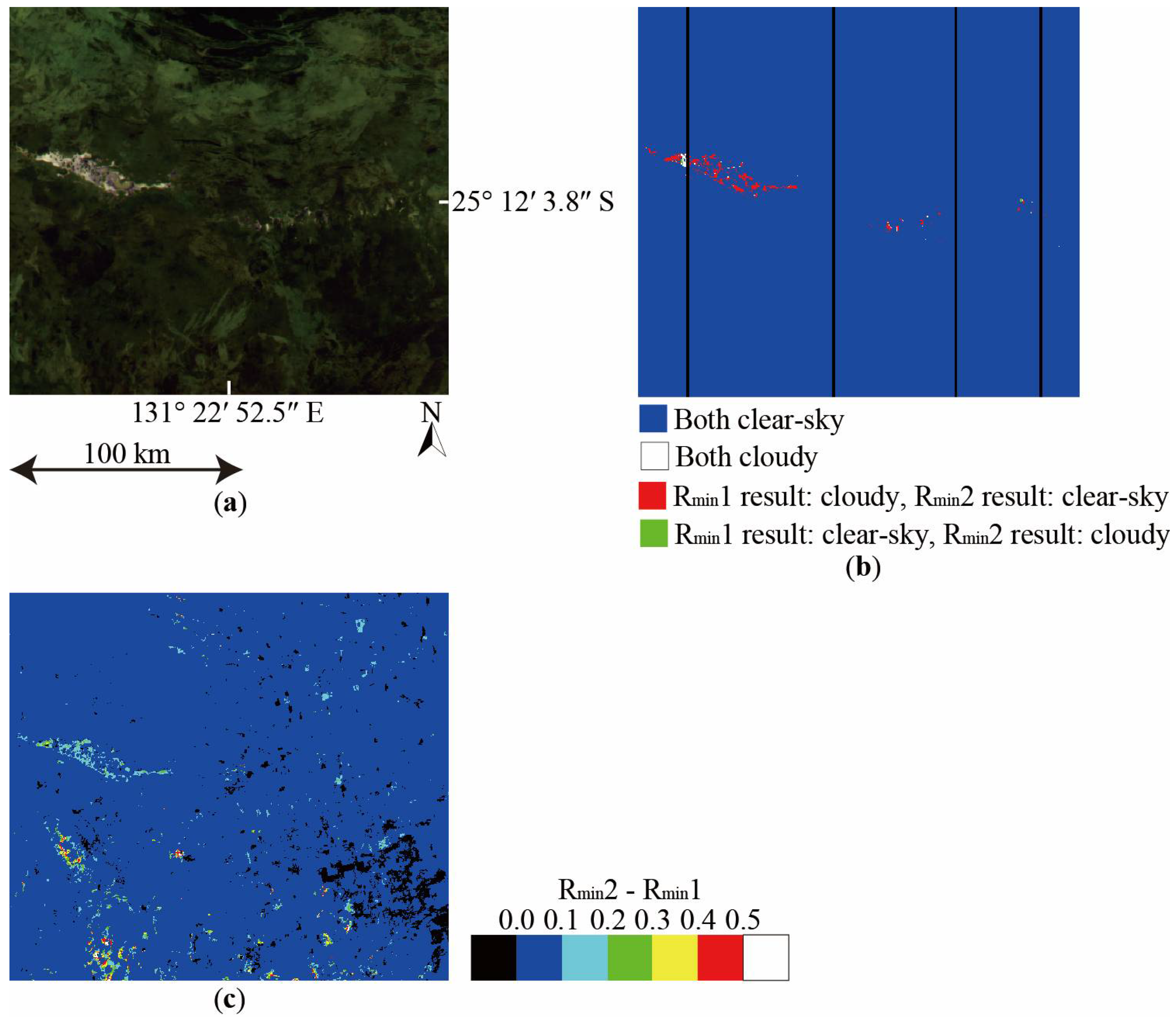
• Water regions near the boundary between land and water where R_min1 results misidentified clouds were improved in R_min2 results.
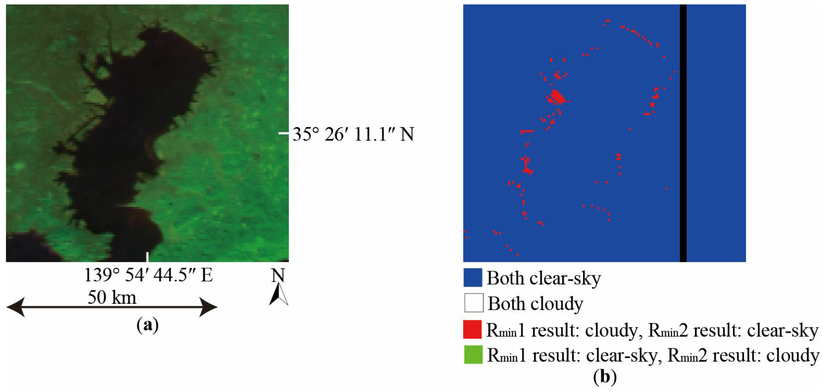
• Furthermore, there were almost no differences between R_min1 results and R_min2 results in water sun-glint regions.

For these reasons, R_min2 results were better than R_min1 results, except for particular situations, e.g., those described in ii and v above.

References

- NIES GOSAT-2 Project. Available online: www.gosat-2.nies.go.jp (accessed on 26 February 2018).
- Ishida, H.; Nakajima, T.Y. Development of an unbiased cloud detection algorithm for a spaceborne multispectral imager. J. Geophys. Res. 2009, 114, D07206. [Google Scholar] [CrossRef]
- Ishida, H.; Nakajima, T.Y.; Yokota, T.; Kikuchi, N.; Watanabe, H. Investigation of GOSAT TANSO-CAI cloud screening ability through an intersatellite comparison. J. Appl. Meteorol. Climatol. 2011, 50, 1571–1586. [Google Scholar] [CrossRef]
- Ishida, H.; Oishi, Y.; Morita, K.; Moriwaki, K.; Nakajima, T.Y. Development of a support vector machine based cloud detection method for MODIS including the adjustability to various conditions. Remote Sens. Environ. 2018, 205, 390–407. Available online: https://www.sciencedirect.com/science/article/pii/S0034425717305138 (accessed on 26 February 2018). [CrossRef]
- Oishi, Y.; Ishida, H.; Nakajima, T.Y.; Nakamura, R.; Matsunaga, T. The impact of different support vectors on GOSAT-2 CAI-2 L2 cloud discrimination. Remote Sens. 2017, 9, 1236. Available online: https://www.mdpi.com/2072-4292/9/12/1236 (accessed on 26 February 2018). [CrossRef]
- Oishi, Y.; Kamei, A.; Yokota, Y.; Hiraki, K.; Matsunaga, T. Evaluation of the accuracy of GOSAT TANSO-CAI L2 cloud flag product by visual inspection in the Amazon and of the impact of changes in the IFOV sizes of TANSO-FTS. J. Remote Sens. Soc. Jpn. 2014, 34, 153–165. Available online: https://www.jstage.jst.go.jp/article/rssj/34/3/34_153/_article (accessed on 26 February 2018). [CrossRef]
- Oishi, Y.; Hiraki, K.; Yokota, Y.; Sawada, Y.; Murakami, K.; Kamei, A.; Yoshida, Y.; Matsunaga, T. Usability evaluation of GPU for GOSAT-2 TANSO-CAI-2 L2 cloud flag processing. J. Remote Sens. Soc. Jpn. 2015, 35, 173–183. Available online: https://www.jstage.jst.go.jp/article/rssj/35/3/35_173/_article (accessed on 26 February 2018). [CrossRef]
- Oishi, Y.; Nagao, T.M.; Ishida, H.; Nakajima, T.Y.; Matsunaga, T. Preliminary study of a method using the GOSAT-2 CAI-2 cloud discrimination for screening of cloud-contaminated FTS-2 data. J. Remote Sens. Soc. Jpn. 2015, 35, 299–306. Available online: https://www.jstage.jst.go.jp/article/rssj/35/5/35_299/_article (accessed on 26 February 2018). [CrossRef]
- Oishi, Y.; Nakajima, T.Y.; Matsunaga, T. Difference between forward- and backward-looking bands of GOSAT-2 CAI-2 cloud discrimination used with Terra MISR data. Int. J. Remote Sens. 2016, 37, 1115–1126. [Google Scholar] [CrossRef]
- Cano, D.; Monget, J.M.; Albuisson, M.; Guillard, H.; Regas, N.; Wald, L. A method for the determination of the global solar radiation from meteorological satellite data. Sol. Energy 1986, 37, 31–39. Available online: https://www.sciencedirect.com/science/article/pii/0038092X86901040 (accessed on 26 April 2018). [CrossRef]
- Ipe, A.; Clerbaux, N.; Bertrand, C.; Dewitte, S.; Gonzalez, L. Pixel-scale composite top-of-the-atmosphere clear-sky reflectances for Meteosat-7 visible data. J. Geophys. Res. 2003, 108, D19. [Google Scholar] [CrossRef]
- Minnis, P.; Harrison, E.F. Diurnal variability of regional cloud and clear-sky radiative parameters derived from GOES data. Part I: Analysis method. J. Clim. Appl. Meteorol. 1984, 23, 993–1011. [Google Scholar] [CrossRef]
- Popp, C.; Hauser, A.; Foppa, N.; Wunderle, S. Remote sensing of aerosol optical depth over central Europe from MSG-SEVIRI data and accuracy assessment with ground-based AERONET measurements. J. Geophys. Res. 2007, 112, D24S11. [Google Scholar] [CrossRef]
- Algorithm Theoretical Basis Documents on the Processing of GOSAT TANSO-CAI L3 Global Reflectance Products. Available online: https://data2.gosat.nies.go.jp/GosatDataArchiveService/doc/GU/ATBD_CAIL3REF_V1.0_en.pdf (accessed on 26 February 2018).
- Shuttle Radar Topography Mission. Available online: https://www2.jpl.nasa.gov/srtm/ (accessed on 26 February 2018).
- U.S. Geological Survey (USGS) Global Land 1-KM Advanced Very High Resolution Radiometer (AVHRR) Project. Available online: https://lta.cr.usgs.gov/AVHRR (accessed on 26 February 2018).
- Fukuda, S.; Nakajima, T.; Takenaka, H.; Higurashi, A.; Kikuchi, N.; Nakajima, T.Y.; Ishida, H. New approaches to removing cloud shadows and evaluating the 380 nm surface reflectance for improved aerosol optical thickness retrievals from the GOSAT/TANSO-Cloud and Aerosol Imager. J. Geophys. Res. 2013, 118, 13521–13531. [Google Scholar] [CrossRef]