Article

A Geostatistical Approach for Modeling Soybean Crop Area and Yield Based on Census and Remote Sensing Data

by
Michel Eustáquio Dantas Chaves
1,*,
Marcelo De Carvalho Alves
1,
Marcelo Silva De Oliveira
2 and
Thelma Sáfadi
2
1
Department of Engineering, Federal University of Lavras, University Campus, P.O. Box 3037, Lavras 37200-000, Brazil
2
Department of Statistics, Federal University of Lavras, University Campus, P.O. Box 3037, Lavras 37200-000, Brazil
*
Author to whom correspondence should be addressed.
Remote Sens. 2018, 10(5), 680; https://doi.org/10.3390/rs10050680
Submission received: 16 March 2018 / Revised: 13 April 2018 / Accepted: 21 April 2018 / Published: 27 April 2018
(This article belongs to the Special Issue Remote Sensing Image Downscaling)

Abstract

:
Advances in satellite imagery and remote sensing have enabled the acquisition of spatial data at several different resolutions. Geographic information systems (GIS) and geostatistics can be used to link geographic data from different sources. This article discusses the need to improve soybean crop detection and yield prediction by linking census data, GIS, remote sensing, and geostatistics. The proposed approach combines Brazilian Institute of Geography and Statistics (IBGE) census data with an eight-day enhanced vegetation index (EVI) time series derived from Moderate Resolution Imaging Spectroradiometer (MODIS) data to monitor soybean areas and yields in Mato Grosso State, Brazil. In situ data from farms were used to validate the obtained results. Binomial areal kriging was used to generate maps of soybean occurrence over the years, and Gaussian areal kriging was used to predict soybean crop yield census data inside detected soybean areas, which had a downscaling effect on the results. The global accuracy and the Kappa index for the soybean crop detection were 92.1% and 0.84%, respectively. The yield prediction presented 95.09% accuracy considering the standard deviation and probable error. Soybean crop detection and yield monitoring can be improved by this approach.

Graphical Abstract

1. Introduction

Advances in satellite imagery and remote sensing now enable scientists to acquire spatial data at several different resolutions [1]. An increase in spatial resolution is known as downscaling. In the context of remote sensing, downscaling refers to a decrease in the pixel size of remotely sensed images [2]. Data also can be downscaled for area-to-point prediction or for areal interpolation, a kriging-based disaggregation technique [3]. Area-to-point prediction uses a downscaling process to predict the same continuous variable at a finer spatial resolution than the input. Once a prediction surface has been created, predictions can be aggregated back to a new set of polygons [2,3].
The issue of scaling is important in various fields, and is one of the most challenging and fascinating aspects of spatial statistics. The choice of an appropriate measurement scale is essential for understanding spatial processes, because mechanisms that are crucial to the spatial dynamics of a process at one scale may be unimportant at another. Relationships between variables at one scale may be obscured or distorted when viewed at another scale [1]. The measurement process involves the important aspect of uncertainty in both sampling and measurement. The sampling process is determined by the support—i.e., the space over which each observation is defined—and the spatial extent; the components of this process are the sampling scheme, the number of observations, and the density of the sample [4]. The support is the parameter of interest in downscaling.
Change-of-support issues are a concern within the field of geostatistics. The change-of-support problem (COSP) refers to the challenge of making a valid inference about a spatial variable at one support based on data at a different support [5]. Most COSPs and their solutions have been concerned with upscaling the prediction of a variable whose support is larger than that of the observed data. Block kriging prediction is commonly used to upscale spatial processes, and is one solution to the point-to-area COSP [5].
In geostatistics, the regularization of the semivariogram changes the support, or measurement scale, of the semivariogram function that is used to describe the structure of spatial variation, without requiring new data on the new support. Changing the support of a variable creates a new variable with different statistical properties. The issue of how the spatial variation in one variable that is associated with a given support relates to that of the new variable with a different support is a change-of-support problem [5].
The modifiable areal unit problem (MAUP) can change the support of soybean crop variables [6], since it is impossible to grow both soybeans and other crops in the same space simultaneously. The MAUP comprises two problems: scale effect and zoning effect. The scale or aggregation effect concerns the different inferences obtained when the same set of data is grouped into increasingly larger areal units. The grouping or zoning effect refers to the variability in results due to alternative configurations of the areal units, leading to differences in unit shape at the same or similar scales.
Geostatistical methods offer an approach to generating the best linear unbiased prediction (BLUP), creating a general method for combining data collected from different geographical units. BLUP can be used to provide a smooth surface of point support based on aggregated data, and make predictions for one set of geographic units based on another set of either nested or overlapping geographic units [5]. This kriging approach accounts for the shape and size of geographical units, accommodates different spatial supports for the data and the prediction without restriction to a single type of areal data at one time, and provides a measure of prediction error variance. Its recent generalization as area-and-point kriging allows the mapping of attribute values within each sampled geographical unit under the constraint that the average of point estimates returns the areal data with coherency [7].
This paper presents an uncertainty approach to the geostatistical mapping of harvested soybean areas and yields in the State of Mato Grosso (MT), Brazil, combining geographic sets of area-based data with remotely sensed data provided by an eight-day Moderate Resolution Imaging Spectroradiometer (MODIS) enhanced vegetation index (EVI) time series. This approach provides a measure of uncertainty in the results, and incorporates relevant covariate information that may be used to improve predictions.

2. Materials and Methods

2.1. Study Area

The study area is the State of Mato Grosso (MT), which is located in the central–west region of Brazil (Figure 1) and covers an area of approximately 905,000 km2. Mato Grosso was chosen for this study because its landscape is heterogeneous, which is a result of an active pioneer frontier shaped by different populations (public and private colonists, logging industries, indigenous societies), land uses, practices, and varying natural conditions (climate, soil, vegetation) [8].
The southern region of the State is a tropical wetland known as the Pantanal (61,000 km2). In the north are the moist forests of Amazonia (484,000 km2). The central region is dominated by vast tropical savannas known as Cerrado (360,000 km2), where agribusiness is concentrated [9]. According to Brown et al. [10], Mato Grosso’s climate (Köppen Aw) is hot—semi-humid to humid—with pronounced seasonality marked by a dry season from May to October. The rainy season occurs from October to May [11]. The climatic gradient is largely coincident with a gradient in land-use change, indicating the interconnectedness of biophysical and socio-economic processes [12]. Many of the State’s soils are old, deep, and nutrient-poor [10]. Nevertheless, these soils have the highest agricultural potential in the country, due to the use of modern agricultural techniques, the development of adapted soybean varieties, and favorable world markets [13]. According to Brazilian Institute of Geography and Statistics (IBGE) [14], the total planted area in Mato Grosso increased by 297% (from 4.74 million to 14.10 million ha) between 2000 and 2015.
By 2000, the widespread use of monoculture rendered the crops highly vulnerable to “Asian rust” (Phakopsora pachyrhizi Sydow & P. Sydow), which is a new soybean disease that appeared during the 2002/2003 harvest. Furthermore, the unfavorable exchange rate between the Brazilian currency (Real) and the United States (US) dollar from 2005 to 2007 highlighted the economic vulnerability of the region’s producers to soybean monoculture [15]. To reduce their vulnerability, the soybean producers changed their agricultural management practices. Since Asian rust makes soybean crops unfeasible between June and September, a soybean host-free period (Vazio Sanitário) was established in 2007. Additionally, a second crop (Safrinha) following the soybean harvest was introduced to prevent soil erosion, improve soil quality, break pest cycles, maintain soil moisture, and set the conditions for high-quality no-tillage operations [16]. This strategy enables growers to take advantage of the long tropical growing season and produce two crops per year [8].

2.2. Data Acquisition and Processing

The Moderate Resolution Imaging Spectroradiometer (MODIS) sensor provides a reliable reflectance time series with acceptable resolution and frequency, showing high potential for large-scale mapping. Two of the most suitable products are MOD13Q1 and MYD13Q1, which are provided every 16 days at a 250-m spatial resolution, presenting the enhanced vegetation index (EVI) and the normalized difference vegetation index (NDVI). These products start on different days (one starts in the middle of the compositing period of the other). This situation effectively creates an eight-day product, which improves temporal change detection [17]. Previous research has successfully used MODIS time series data as an input to classify land cover types [10,16,18,19] and monitor the soybean crops in Mato Grosso [11,20,21] over the last decade. Due to the singular characteristics of the soybean-producing farms in the State, the MODIS data, with a near daily temporal resolution and 250-m spatial resolution, can be considered as adequate for crop mapping.
Between the EVI and NDVI vegetation indexes, the EVI was chosen due to its potential to reduce atmospheric and soil background effects [22]. Different studies, such as Zhu et al. [20] and Zhong et al. [23], consider EVI to be the most suitable index to represent crop growth with sufficient sensitivity in high biomass periods, especially for soybean discrimination during maximum crop development. According to Risso et al. [18], the EVI performs the best for soybean discrimination during the crop seasons in Mato Grosso, while the NDVI is unfit for this objective. The EVI time series profiles gradually increase as the vegetative growth stage progresses over time; it reaches the peak value on the heading date, and then begins to decline in the reproductive growth stage until the mature crop is harvested [24]. The EVI is determined by:
EVI = G ( ρ N I R ρ r e d ) ( ρ N I R + C 1 ) ( ρ r e d C 2 ) ( ρ b l u e + L )
where the ρ values are partially atmospherically corrected (Rayleigh and ozone absorption) surface reflectance; L is the canopy background adjustment (L = 1), C1 and C2 are coefficients of the aerosol resistance term that uses the blue band (458–479 nm) of MODIS to correct for aerosol influences in the red band (C1 = 6 and C2 = 7.5), and G is a gain factor (G = 2.5) [25].
However, some limitations may occur when attempting to apply this approach to the large-scale classification and monitoring of crops [16,20,24]. The EVI time series generated from the MODIS surface reflectance data include various noise components, such as aerosols and bidirectional reflectance distribution factors; thus, it is necessary to reprocess these data to remove the noise components before using them to discriminate crop growth profiles [24]. The MOD13Q1 and MYD13Q1 have quality assessment (QA) fields that indicate cloud state and snow/ice presence; these quality control fields are divided into VI Quality and Pixel Reliability, respectively. This information allows MODIS database users to verify the reliability of a pixel in relation to the atmospheric conditions (clouds, ozone, dust, and other aerosols), and check the bidirectional effects related to data acquisition geometry (source–target–sensor) and possible failure of instruments or data processing methods [26]. In this paper, the EVI data were obtained from the United States Geological Survey’s Land Processes Distributed Active Archive Center (LP DAAC) [27]. We acquired one MODIS tile (h12v10), which covered all of the main soybean cultivation areas. The images were re-projected into GeoTIFF format, using the MODIS Reprojection Tool [27]. The QA fields were used to eliminate noisy pixels.

2.3. Proposition of the Soybean Enhanced Index SEI P i x e l

The EVI images obtained for each crop season were chronologically organized. We then proposed a calculation of the total change magnitude per pixel, called the Soybean Enhanced Index ( SEI P i x e l ) . The Euclidean distance between endpoints (dates 1 and 2) was calculated based on the change in dimensional space characterized by the MODIS EVI tile h12v10 for each crop season, according to Equation (2), which was modified from Jensen (2005):
SEI P i x e l = g = 1 n [ EVI i j k ( d a t e   2 ) EVI i j k ( d a t e   1 ) ] 2
where i and j are the latitude and longitude of the two-dimensional space of each MODIS tile, and EVI i j k ( d a t e   1 ) and EVI i j k ( d a t e   2 ) are the values of dates 1 and 2 in EVI band k, for the n seasonal growth profile.
For this procedure, the in situ data were stratified according to the sowing date described for each crop field. The EVI dates 1 and 2 refer respectively to the minimum and maximum vegetative vigor of soybean in a seasonal growth profile.
The SEI P i x e l for each crop season was classified into binary (0 and 1) values, where 0 and 1 were “Non-soybean” and “Soybean” cropland, respectively. The threshold values for the classification were defined based on the time series responses and on the Brazilian Institute of Geography and Statistics (IBGE) survey of soybean crop production and harvested area [28] for all of the crop seasons in all of the Mato Grosso municipalities. The harvested soybean crop areas estimated by the SEI P i x e l were recorded and compared with the IBGE survey, defining the best threshold values based on the highest similarity between the “Soybean” and “Non-soybean” cropland classification results of both surveying methods.
The Mato Grosso municipalities vector boundaries—2007 reference year, 1:2,500,000 scale, SIRGAS 2000 geographic latitude and longitude—were obtained from IBGE [14]. The vector boundaries were converted to WGS84 geographic latitude and longitude. The vector boundary zones for each of the 141 municipalities corresponded to the harvested area and yield data obtained for the 2000/2001 to 2011/2012 crop seasons. Zonal statistics were used to calculate the number of soybean crop pixels, according to the SEI P i x e l , inside each vector boundary zone of the 141 municipalities.
The intensification of soybean cropland in Mato Grosso, per pixel ( iSEI P i x e l ) , was computed by summing the ( SEI P i x e l ) binary images (0 or 1) for the n crop seasons, generating information about the number of years harvested (Equation (3)):
iSEI P i x e l = n ( SEI P i x e l   i j k )
The R-squares goodness of fit criteria, which were derived from the polynomial regression linear fit, were used to compare the classified results of the ( SEI P i x e l ) and IBGE [28] data.

2.4. Geostatistical Analysis

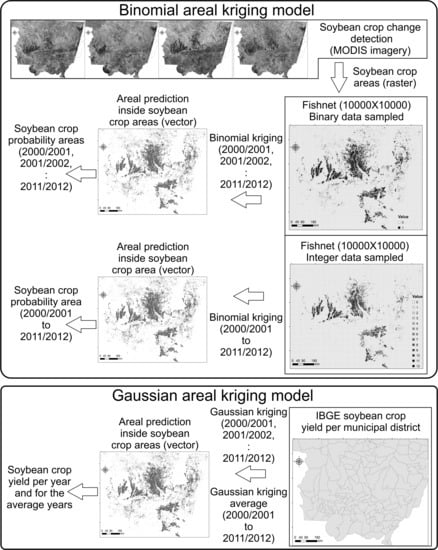
2.4.1. Binomial Areal Kriging Model

The Mato Grosso region (D) was composed of N areas determined by a vector that was used to sample the SEI P i x e l imagery for each evaluated crop season, and the iSEI P i x e l imagery for all of the crop seasons collectively. The sampled pixels of the SEI P i x e l imagery were classified as either “Non-soybean” (0) or “Soybean” (1) binary values. In the iSEI P i x e l imagery, each pixel was assigned a value between 0–12, where 12 represented the agroecosystems cultivated with soybean crops for 12 consecutive years. The value of the soybean crop areas and the total quantity of soybean crop areas were denoted by l(ui) and n(ui), respectively. The vector of spatial coordinates ui = (xi, yi), i = 1, ..., N, was georeferenced to the centroid of the i-th area. The random variable Z(ui) was the percentage of soybean crop area occurrence, and one of the realizations of Z(ui) was z(ui), which was defined by l(ui)/n(ui).
Soybean crop areas within region A were assumed to be influenced by an underlying event—denoted by R(u)—that was caused by a stochastic process { R ( u ) , u D 2 } , where R(u) was a random variable with continuous variation and correlation over space and whose values were not directly observed. Therefore, there are two distinct geographic supports. The first relates to the geographic areas inside region D, with z(ui) observed values of the random variable Z(ui). The second relates to the nature of the evaluated process, which was characterized by the continuous surface R(u). Considering R(ui), i = 1, ..., N, the average event associated with the centroid of the i-th geographical support of the area vi is defined by [29]:
R ( u i ) = 1 v i v i R ( u ) d u
The R(ui) values are associated with the percentage of occurrence of the event P(ui) in the i-th geographical support area vi, in the time interval δt [30]:
R ( u i ) = P ( u i ) δ t
where for δt = 1, R(ui) = P(ui).
The random variable L(ui) relates to the number of occurrences of the event in n(ui) repetitions of the i-th geographical support and presents binomial distribution as:
L ( u i ) ~ B i n [ r ( u i ) , n ( u i ) ]
where Bin denotes a binomial distribution, the parameter r(ui) = p(ui), and n(ui) is the total quantity of soybean crop areas in the i-th geographical support.
The different cases of the risk of occurrence of soybean crop areas are independent when R(u) is fixed, because R(u) is the only source of correlation between the cases. Thus, the observed rates are variables with distribution [29]:
Z ( u i ) | R ~ 1 n ( u i ) B i [ r ( u i ) , n ( u i ) ]
The following conditional moments can be established based on Equation (7) [3]:
E [ Z ( u i ) | R ] = R ( u i )
E [ Z 2 ( u i ) | R ] = n ( u i ) 1 n ( u i ) R 2 ( u i ) + R ( u i ) n ( u i )
E [ Z ( u i ) Z ( u i ) | R ] = R ( u i ) R ( u i )
The semivariogram of the binomial kriging was established based on the conditional moments [29]:
γ ( u i , u j ) R = γ ( u i , u j ) Z 1 2 { 1 n ( u i ) + 1 n ( u j ) } μ ( 1 μ ) + 1 2 { σ R ( u i ) 2 n ( u i ) + σ R ( u j ) 2 n ( u j ) } E [ Z ( u i ) Z ( u i ) | R ] = R ( u i ) R ( u i )
where γ ( u i , u j ) R = 1 2 E [ R ( u i ) R ( u j ) ] 2 and is defined as the semivariogram function of the risk of soybean crop area occurrence; γ ( u i , u j ) Z = 1 2 E [ Z ( u i ) Z ( u j ) ] 2 is the semivariogram function of the rates; and n(ui) and n(uj) are the total number of soybean crop areas in the i-th and j-th geographic supports, with centroids in ui and uj, respectively. The average risk µ is E[R(u)]. The risk variances in the i-th and j-th geographic supports are σ R ( u i ) 2 and σ R ( u j ) 2 , respectively. If the variogram is bounded by a finite value γ(∞), a covariance function can be found, such as [31]:
C ( u ) = γ ( ) γ ( u )
When an experimental variogram exhibits a sill, it can be fit to a theoretical variogram that is a covariance function C(u), and based on the formula for bounded variograms [31]:
γ ( u ) = C ( 0 ) C ( u )
where C(u) is the stationary covariance and C(0) = Var{Z(u)} is the value at the origin of the covariance function.
The risk R(u) was estimated based on the information of Z(ui). Binomial kriging was done based on the direct covariance between Z(ui) and Z(uj). Binomial kriging in an unknown location u0 was estimated by a linear combination of neighbor rates z(ui) [32]:
R ^ ( u 0 ) = i = 1 N λ ( u i ) z ( u i )
where z(ui) is the rate observed in the i-th geographical support with a centroid in ui, N is the total number of centroids used in the calculus of R ^ ( u 0 ) , and λ ( u i ) is the weight attributed to the i-th observation of z(ui).
The λ ( u i ) was determined according to the spatial correlation of the risk and the properties of non-bias and minimum variance. Non-bias implies that the difference between the estimated value and the true value at the same point must be null:
E [ R ^ ( u 0 ) R ( u 0 ) ] = 0
E [ i = 1 N λ ( u i ) z ( u i ) R ( u 0 ) ] = 0
E i = 1 N λ ( u i ) E [ z ( u i ) ] E [ R ( u 0 ) ] = 0
E i = 1 N λ ( u i ) μ μ = 0
μ [ i = 1 N λ ( u i ) 1 ] = 0 i = 1 N λ ( u i ) = 1
The non-bias property requires that the sum of the weights equals 1.
The minimum variance property means that the estimator has minimum variance when compared to other linear estimators:
σ R ( u 0 ) 2 = E { [ R ^ ( u 0 ) R ( u 0 ) ] 2 }   is   minimal
Equation (18) must be minimized under the restriction that i = 1 N λ ( u i ) = 1 . Minimization is achieved using Lagrange techniques. Minimizing σ R ( u 0 ) 2 , the weights were obtained by applying [29]:
{ i = 1 N λ ( u i ) C ( u i , u j ) Z + φ = C ( u j , u 0 ) Z R   for   all   j = 1 , , N i = 1 N λ ( u i ) = 1
where C ( u i , u j ) Z is the covariance of the frequencies, and C ( u j , u 0 ) Z R is the covariance between frequency and risk. The covariance depends not only on the spatial separations, xixj, between the centroids of the fishnet, but also on the number of soybean crop areas therein. φ is the Lagrange multiplier.
The dispersion around the resulting estimate of risk, or the kriging variance, was obtained by [32]:
σ ^ R 2 ( u 0 ) = C ( 0 ) Z i = 1 N λ ( u i ) C ( u i , u 0 ) Z R + φ = C ( 0 ) R i = 1 N λ ( u i ) C ( u i , u 0 ) R + φ   if   i 0
The binomial kriging prediction values depend on the structure of the semivariogram or the covariance function.

2.4.2. Gaussian Areal Kriging Model

The soybean crop yield model does not observe a realization of the point-level process, Z(s), but instead uses census data (B) pertaining to the 141 vector boundaries of the Mato Grosso municipalities, Z(B) = (Z(B1), ..., Z(Bn))′, and the prediction of Z(A) is of interest. The A can be general, leading to several different types of change-of-support problems. For example, when Bi values are points instead of areas and Ai values are areas, the point-area change-of-support problem arises. If Ai values are points and Bi values are areas, then the problem becomes one of the spatial disaggregation, an area-to-point COSP, requiring the prediction of a spatial intensity function from aggregated data. Ai and Bi may be different geographic regions at the same spatial scale or different spatial scales. In such cases, A may be wholly contained in one of the Bi, or it may overlap with two or more of the B units. Thus, the best linear unbiased predictor had the form [5]:
Z ^ ( A ) = w ( A ) Z ( B ) ,   with   w ( A ) = ( w 1 ( A ) , , w n ( A ) )
where each weight wi(A) measures the influence of datum Z(Bi) on the prediction of Z(A).
Gotway and Young [5] provides the optimal weights, as follows:
w u = ( u ) 1 σ u
where wu = (w1(A), ..., wn(A), m′)′ ≡ (w(A)′m′)′, and m is a (p × 1) vector of Lagrange multipliers.
The (n + p) × (n + p) matrix Σu is based on the data and covariates of the B units [5]:
u = [ B B x ( B ) x ( B ) ϕ ]
The elements of the (n × n) matrix ΣYY are the (Bi, Bj) covariance:
C ( B i , B j ) = cov ( Z ( B i ) , Z ( B j ) ) = 1 | B i | 1 | B j | B i B j C ( u v ) d u d v
The matrix σu comprises information on the A units, as well as their spatial relationships to the B-units, and is equal to:
u = [ σ A B x ( A ) ]
where the elements of the (n × 1) vector σAB are the (A, Bi) covariance:
C ( A , B i ) = cov ( Z ( A ) , Z ( B i ) ) = 1 | A | 1 | B i | A B i C ( u v ) d u d v
The (p × 1) vector x(A) comprises the covariate information associated with A, x(A) = (x1(A), x2(A), ..., xP(A))′ [5].
Gotway and Young [5] sets forth the corresponding mean-squared prediction errors:
σ A A w u σ u
with σAA = cov(Z(A), Z(A)).
The measurement error in the data Z(Bi) can be accommodated by assuming that:
Z ( B ) = B Z ( s ) d s + ε ( B )
in addition to using a filtered version of this predictor [5,33].
When it is necessary to predict Z(s) associated with a point s using data Z(B), the predictor becomes:
Z ^ ( s ) = i = 1 N w i ( s ) Z ( B i )
The weights wi(s) can be obtained using Equation (24) with σu replaced by [σsBʹ x(s)ʹ ]ʹ, where σsB is the (n × 1) vector with ith element cov(s, Bi).
The relationship between the semivariogram associated with Z(B) and the one associated with the underlying point-support process, Z(s), is given by Cressie [33] and Gotway and Young [5]:
2 γ ( B i , B j ) var ( Z ( B i ) Z ( B j ) ) = 1 | B i | | B i | B i B i γ ( s u ) 1 | B j | | B j | B j B j γ ( s u ) d s d u + 2 | B i | | B j | B i B j γ ( s u ) d s d u
where γ(su) = (1/2)var(Z(s) − Z(u)) is the semivariogram of the point-support process {Z(s)}.
The binomial and Gaussian kriging implementations were synthesized in Figure 2.

2.4.3. Block Kriging Model

The prediction results of the binomial and Gaussian areal kriging at locations with point support were predicted in the soybean crop areas detected by remote sensing. The percentage of soybean crop occurrence and yield were predicted by block kriging, which was used to predict the average value of the process at a larger scale, accounting for not only the size but also the shape and orientation of volume B. The prediction of the spatial average from point-support measurements Z(s1), Z(s2), ..., Z(sn) was:
Z ( B ) = 1 | B | B Z ( s ) d s
The set B is a soybean cropland region that forms the spatial support of Z(B). The resulting predictor is given by:
Z ^ ( B ) = i = 1 N w i Z ( s i )
The optimal weights (wi) were obtained by applying [5,33,34]:
i = 1 N w k C ( s i , s k ) + j = 1 P m j x j ( s i ) = C ( B , s i ) i = 1 , , N j = 1 P w i x j ( s i ) = x j ( B ) j = 1 , , P
where x j ( B ) = 1 | B | B x j ( u ) d u , j = 1 , 2 , , p ; mj represents the Lagrange multipliers from the constrained minimization, and C(B, si) is C ( B , s i ) = cov ( Z ( B ) , Z ( s i ) ) = B C ( u , v ) d u d v / | B | .
The advantage of predicting Z(B)—rather than predicting Z(uj) for many points uj in B and averaging the resulting predictions—is the ease of obtaining an uncertainty measure of the resulting predictor. The mean-squared prediction error associated with Z ^ ( B ) was [5,33,34]:
C ( B , B ) i = 1 N C ( B , s i ) j = 1 P m j x j ( B )
where C ( B , B ) = 1 | B | 2 B B C ( u v ) d u d v .
The point-to-point covariance function, C(uv), is assumedly known for theoretical derivations, but is estimated and modeled with a valid positive definite function based on the point-support data.

2.4.4. Modeling Semivariogram and Covariance Function

The estimation of the covariance terms in the kriging system requires knowledge of the point-support covariance or point-support semivariogram model. Given the availability of areal or polygon data only, it was necessary to compute and model the variogram of the areal data and deconvolute the block-support model to derive the point-support semivariogram. The point-support variogram was inferred using iterative deconvolution [35]. An experimental semivariogram and a covariogram were computed and then modeled by a weighted least-squares fitting procedure. A candidate point-support model, or deconvoluted model, was then chosen and regularized. The regularized model was then compared to the model fitted to the experimental variogram of the areal or polygon data. Based on the differences between the regularized model and the areal model, the optimal point-support model was rescaled, providing a new candidate model for the next iteration. The deconvoluted model was closest to the model for the areal data, and was used for the area-to-point kriging. This procedure considered the irregular shape and size of areal units [36].
Each polygon was overlaid with a square lattice, and a point was assigned to each intersection in the lattice to produce the semivariogram or covariance function. The lattice spacing parameter specifies the horizontal and vertical distance between each point. The horizontal axis of the semivariogram or covariance function presents the average distance between the polygons, which was calculated using the cells of the overlapping grid. The crosses represent the empirical semivariances, or covariance values, which were calculated using the available averaged data for the polygons.
The line is the estimated point semivariogram or covariance function models. The bars are the confidence intervals, which are calculated assuming re-estimated empirical semivariances or normally distributed and uncorrelated covariance. For the properly specified semivariogram or covariance model, 90% of the empirical covariance is expected to fall within the confidence intervals, indicating that the model fits the data and that the results can be trusted. The line of the semivariogram model might not pass through the confidence intervals, but this is not a problem, and the criteria for a good model does not change. If a large percentage of the empirical semivariances fall within the confidence intervals, the areal kriging can produce more accurate predictions and prediction standard errors than point kriging, with values assigned to the centroids of polygons [3].
The stable covariance function and semivariogram models were used to characterize the soybean harvested areas and yields, respectively. The stable model has the same behavior near the origin and reaches a sill [34]:
C ( u ) = b exp ( ( u a ) α )   ( a > 0 ,   0 < α 2 ,   b > 0 )
where b is the sill, a is the range, and α is the parameter.
Wackernagel [31] determines the stable semivariogram model:
γ ( u ) = b ( 1 exp ( | u | α a ) )   ( a > 0 ,   0 < α < 2 ,   b > 0 )

2.5. Validation Phase

The in situ data were kindly provided by the farmers of five visited agglomerates. This data referenced the cultivation practices applied at the crop field level in the 2010/2011 crop season, and included: variety, sowing, germination, and harvesting dates, soil texture, total planted area, and the number of 60-kg bags of harvested crop per hectare (ha) of each crop field. The 2010/2011 crop season was chosen for analysis because it sustained minimal impact from climatic variations caused by La Niña (rainfall reduced) or El Niño (excessive rainfalls) [37], which are phenomena that directly affect Mato Grosso, causing losses in yield [38].
The soybean crop expansion occurred in four main agricultural regions: (1) along the BR-163 highway that links Cuiabá to Santarém (State of Pará); (2) on the Parecis plateau, in the western region, including Sapezal and Diamantino; (3) the eastern region, near Santo Antônio do Leverger and Querência; and (4) the southeastern region, near Rondonópolis and Primavera do Leste. In this context, five agglomerates with high soybean production were chosen for the validation: Vale do Rio Verde (northern region, in Tapurah/Ipiranga do Norte); Santa Luzia and Colorado (western region, in Sapezal and Diamantino, respectively); Malu (eastern region, in Bom Jesus do Araguaia/Ribeirão Cascalheira); and Colibri (southeastern region, Santo Antônio do Leverger) (Figure 3).

2.5.1. Soybean Crop Area Validation Phase

Punctual crop field analyses were applied to verify the accuracy of the SEI P i x e l mapping. To validate the “Soybean” class, one point was chosen from each crop field, totaling 386 samples. To validate the “Non-soybean” areas, the TerraClass land use/land cover map of 2012 [39] was used. TerraClass is a partnership between the National Institute for Space Research (INPE) and the Brazilian Company for Agricultural Research (EMBRAPA) that aimed to classify land use and occupation in the deforested areas of the Legal Amazon. The TerraClass map had the same number of sampling points, but these points were distributed in “Non-soybean” areas. The classification was assessed using an error matrix, overall accuracy, and Kappa statistics [40].

2.5.2. Soybean Crop Yield Validation Phase

To effectuate downscaling at the crop field level, the validation of soybean crop yields involved the verification of the soybean crop yield for each crop field in the agglomerates relative to the yield predicted for 2010/2011, computing the number of 60-kg bags obtained per ha−1. For this, each soybean crop field detected on the farms was sampled once, and the yields obtained from the in situ data were compared with the map of yield classes generated by the Gaussian areal kriging model. For each crop field, the total number of 60-kg bags of soybean harvested per ha−1 at the end of the harvest period was recorded and compared with the prediction. The results were presented in five classes of 60-kg bags per ha−1: less than or equal to 0, from 0.1 to 25, from 25.01 to 45, 45.01 to 55, and equal to or greater than 55.1.
The approach adopted in this study is synthesized in Figure 4.

3. Results

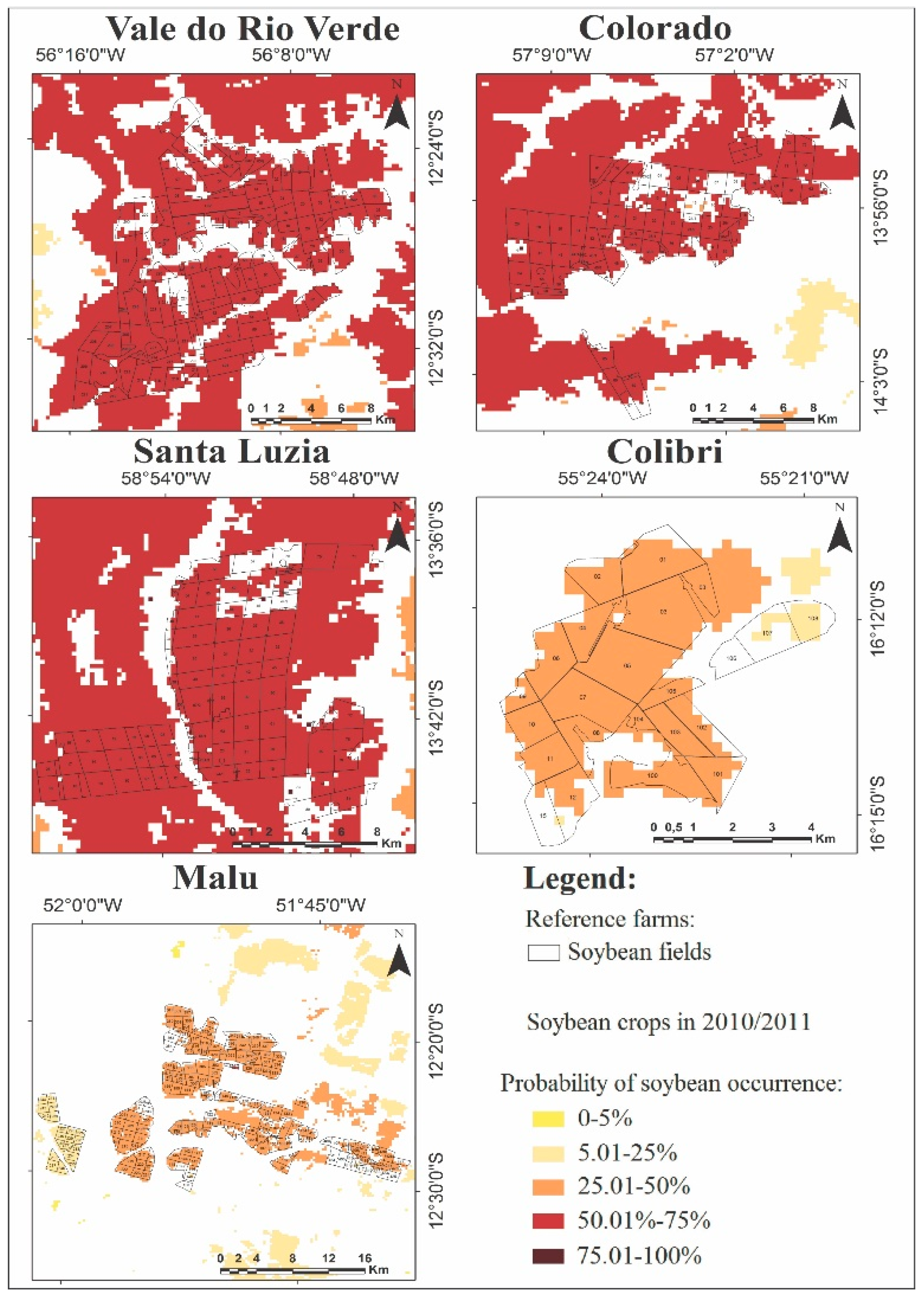
3.1. Soybean Crop Area Results

The SEI P i x e l enabled the detection of soybean harvested areas when compared with IBGE data for the municipalities of Mato Grosso. The regression models between the SEI P i x e l and IBGE presented strong correlations, which were represented by R2 values above 93% (Figure 5).

Binomial Areal Kriging Model for Soybean Crop Area Identification

The covariance function described how soybean harvested areas vary, on average, in Mato Grosso. Since the spatial variability does not change with direction, omnidirectional covariograms were computed, and stable models were fitted using the least-square algorithm (Figure 6).
The values for the binomial kriging equations were obtained based on the mathematical expression of the covariance function. The kriging equations, the estimated percentage of soybean crop areas, kriging variance, and standard errors were solved. Then, the binomial kriging results were predicted for the soybean harvested vector areas detected by remote sensing using block kriging. The maps were classified into percentage of occurrence classes (Figure 7).
The kriging errors were mapped in the same way as the percentage of soybean crop areas. In general, the errors associated with the estimates were small. The largest errors, which were those above 3%, occurred mainly in sparse rural areas; however, highly aggregated areas in regions of Sorriso, Lucas do Rio Verde, Nova Mutum, Nova Maringá, and Sapezal also presented errors above 3%. The periods 2006/2007 and 2010/2011 presented low errors in the sparse rural areas. The period 2010/2011 also presented low errors in highly aggregated soybean crop areas (Figure 8).

3.2. Accuracy Assessment of Soybean Crop Area Results

The SEI P i x e l classification accuracy was evaluated by the analysis of the soybean mapping and the 2010/2011 in situ checkpoint data (Table 1).
The absolute identification of other land uses as being “Soybean” occurred on a major scale, which was possibly due to the similarity in temporal behavior between soybean and other summer crops such as cotton and corn, which were well represented in the region. Subsequently, an accuracy assessment of soybean classification was conducted using the reference data (Table 2).
The SEI P i x e l classification was compared with in situ data in the analysis of the spatial distribution of the probability of soybean occurrence in the agglomerates Vale do Rio Verde, Colorado, Santa Luzia, Colibri, and Malu in the 2010/2011 crop season (Figure 9).

3.3. Soybean Crop Yield Results

Gaussian Areal Kriging Model for Yield Prediction

While the covariance function has described the variation among the soybean-harvested areas in Mato Grosso, the semivariogram can also be used to describe soybean crop yield throughout the space. Omnidirectional semivariograms have been computed using stable models fitted by the least-squares algorithm. The deconvoluted point semivariogram (line) differed from the estimated empirical semivariogram values for the polygons. In this case, areal kriging, in which values are assigned to polygons, can produce more accurate predictions and fewer prediction standard errors than point kriging. Almost all of the re-estimated empirical semivariogram values for polygons (crosses) were inside the 90% confidence intervals (vertical lines) (Figure 10).
The Gaussian areal kriging results were predicted for the soybean harvested vector areas that were detected by remote sensing using block kriging. The highest yield occurred not only in the aggregated soybean crop areas but also in sparse rural areas. However, major producer areas represented a higher proportion of the total yield, and those with smaller areas represented a lower proportion of the total yield. The major producer-aggregated areas presented high yields, particularly in 2010/2011 (Figure 11).
Yield predictions with the most uncertainty did not necessarily correspond to units with low-yield predictions, but the smallest uncertainty values tended to be associated with the predicted high-yield regions (Figure 12).

3.4. Accuracy Assessment of Soybean Crop Yield Results

A comparison of yield estimates (60-kg bags per ha−1) for each agglomerate and the in situ data is presented in Table 3.
Given the limitations, the standard deviation component derived from the interpolation (Equation (40)) is evaluated [41]:
E 50 = ± 0.6745 . σ
The probable error was considered in the yield evaluation, because the defined yield classes do not include the extensive crop fields for which the high yield was approximated. The soybean crop yield prediction analysis was improved by accounting for the probable error (Table 4).
The spatial distribution of the soybean crop yield in the agglomerates Vale do Rio Verde, Colorado, Santa Luzia, Colibri, and Malu in the 2010/2011 crop season (Figure 13) highlights the predominance of the soybean crop in the agricultural regions of Mato Grosso.

4. Discussion

4.1. Soybean Crop Area Results

Gusso et al. [42] used MODIS EVI images from the soybean-sowing period in Mato Grosso to observe their approximated thresholds (Figure 5). Arvor et al. [8], using MODIS EVI for crop mapping in Mato Grosso, observed accuracies higher than 95% in 2006/2007. Risso et al. [18], evaluating MODIS EVI and NDVI for soybean crop area discrimination, also observed a satisfactory application of EVI images from the maximum crop development period for soybean classification in Mato Grosso. Similarly, Souza et al. [43] noted that an EVI time series could be compared to official data to identify soybean croplands. For Victoria et al. [44], estimates based on MODIS vegetation indices presented good agreement with large cultivated areas, but poor agreement with municipalities with small cropland areas. These studies used 16-day composites derived only from MOD13Q1 images. In contrast, we used eight-day composites derived through combining the MOD13Q1 and MYD13Q1 images. Furthermore, the aforementioned studies did not consider large-scale interannual variations resulting from the agricultural dynamics in Mato Grosso. We address this issue with the proposed SEI P i x e l , which covers the phenological cycle of the crop through the 2000/2001 to 2010/2011 crop seasons. The analysis of eight-day rather than 16-day composites, as well as the consideration of large-scale interannual variations, allows the detection of subtle spectral–temporal differences between crop types, improving the method’s crop area identification.
Although IBGE data were used as a reference, the high correlation between the estimates generated by the SEI P i x e l and the IBGE data for some municipalities indicates that the sampling may not accurately represent the IBGE estimate. In this respect, adopting a more reliable reference, with satellite image mapping at greater spatial detail, allowed us to determine the level of uncertainty in the objective and subjective methods of crop forecasting. We were able to ascertain the planted soybean area at the end of the crop development cycle but before harvest, unlike the IBGE survey, which extends beyond the end of the harvesting period.
The intensification of soybean cropland was described by the iSEI P i x e l . The minimum and maximum iSEI P i x e l values were 0 and 12, respectively. Based on the chosen threshold values, SEI P i x e l overestimated the total soybean harvested areas when compared with the IBGE data. Due to the impossibility of determining the real soybean harvested area in Mato Grosso, the use of binomial kriging was necessary to measure the uncertainty in the estimates.

Binomial Areal Kriging Model

The binomial areal kriging results show the soybean expansion in Mato Grosso. Kastens et al. [9] evaluated soybean cultivation in Mato Grosso during 2001 and 2014 in relation to the Soy Moratorium initiative, finding the deforestation rate in the pre-Soy Moratorium period to be more than five times the post-Soy Moratorium rate, while simultaneously observing the pre-Soy Moratorium forest-to-soy conversion rate to be more than twice the post-Soy Moratorium rate. Gibbs et al. [45] observed that, in the two years prior of the agreement, almost 30% of the soybean expansion had occurred through deforestation. After the Soy Moratorium, this value decreased to 3% in the Amazon biome until 2011. These observations indicate that the Soy Moratorium played a role in reducing both deforestation and the subsequent use of the land for soybean production. However, the authors considered that, in the Cerrado biome, where the Soy Moratorium does not apply, the annual rate of soybean expansion over native vegetation areas has remained high, varying from 11% to 23% between 2007 and 2013, demonstrating that the Cerrado is less protected by environmental laws than the Amazon rainforest.
This information corroborates the results obtained by the SEI P i x e l index. An analysis of the maps of each crop season shows that the soybean crop areas expanded mostly in the Cerrado biome. Figure 7 illustrates that the expansion of the soybean crop areas occurred in the four main agricultural regions cited above in item 2.5. The same scenario was found by Gusso et al. [11], Arvor et al. [46] and Dubreuil et al. [47]. In these four agricultural areas, located in the Cerrado biome, the crop identification showed that soybean is the main crop.
Regarding the Amazon biome, region (1) presented soybean expansion in forest areas. This deforestation can be explained by the direct influence exerted by the BR-163 (the main route between the north and south regions of Mato Grosso and principal access road to the Santarém port) on the regional landscape change [47]. According to Morton et al. [48], the improvements of the roads network and the construction of grain storage facilities in northern Mato Grosso have encouraged the direct conversion of forest to soybean crops. To circumvent the Soy Moratorium, the deforested areas in this region were first converted to pasture before being used for soybean production [16,37,47].
Considering that the spatial structure of the soybean areas in Mato Grosso shows that soybean crops are spatially correlated, and that the correlation of the underlying probability of soybean occurrence extends by about 180 km on average, the binomial kriging results mean that soybean crop areas and the uncertainty in their prediction can be mapped geostatistically. The maps show that sparse rural areas present lower percentages of soybean occurrence than the highly aggregated soybean crop areas. Using binomial kriging, we combined different types of geographical units and various sources of information to create maps illustrating where the percentage of soybean harvested areas varied continuously in the space, thereby reducing the visual bias associated with the interpretation of the classified vector maps. By measuring the variance of the prediction errors, we identified large and sparse areas where the estimates were less reliable.
Binomial kriging can be considered a noise filter for generating maps of regional patterns, such as information about the concentration of soybean-harvested areas. This result can be observed in the map of the averaged years, where sparse areas present a low probability of soybean occurrence, due to less agricultural intensification over the years, compared to consolidated agroecosystems (Figure 7). Galford et al. [19] used a wavelet analysis of eight-day MODIS time series data as a filtering approach to detect crops in Mato Grosso, but they left a gap in relation to the determination of uncertainties. The binomial kriging results are promising for the determination of spatial prediction uncertainties as well as for soybean mapping.

4.2. Accuracy Assessment of Soybean Crop Area Results

The comparison between the reference data and the classification of soybean crop areas for the 2010/2011 crop season indicated high alignment. The global accuracy and the Kappa index obtained from the error matrix were 92.1% and 0.84% for the soybean crop, respectively. According to Foody [49], a global accuracy higher than 85% is desirable. However, according to the levels of agreement of Kappa index values proposed by Landis; Koch [50], a classification above 0.80 is considered excellent and highly aligned with the in situ data. On the basis of these indices, the classification could be considered excellent, which indicates the potential for the identification of soybean crop areas in Mato Grosso. These results confirm the potential for using eight-day MODIS EVI composites with geostatistical techniques to map soybean crops.
The values we obtained were even more significant when compared with studies that used data from the same sensor. Arvor et al. [8], using only the MOD13Q1 (16-day time series) to evaluate soybean crop expansion in the vicinity of protected areas in Mato Grosso, obtained 74% global accuracy and a Kappa value of 0.675. Lamparelli et al. [51] obtained Kappa values between 0.60 and 0.80 when estimating soybean crop areas with MODIS data. The values we obtained for user and producer accuracy were also considered excellent. The omission errors were 0.05 for the “Soybean” class, and 0.11 for the “Non-soybean” class. Nevertheless, the commission errors were 0.10 for “Soybean” and 0.05 for “Non-soybean”. Epiphanio et al. [52], using the spectral–temporal response surface (STRS) method for soybean classification in Mato Grosso, obtained omission errors of 0.06 and commission errors of 0.17 for the soybean class, as well as 80% global accuracy and a Kappa value of 0.26, with 343 checkpoints.
The detected errors can be explained by both in situ and orbital data. The in situ data reveals that the distribution of some crop fields is not representative in terms of yield in edge areas bordering other land uses. Therefore, their temporal values of maximum and minimum EVI, amplitude, and mean and standard deviation, are different to the medium and high-yield crop fields. With the mixed response resulting from spectral mixing between different land uses, these crop fields tended to fall below the threshold that is used to define the “Soybean” class, and were thus considered by the classification algorithm as within the “Non-soybean” class. Another important factor is the spatial variability of agricultural calendars. Due to the large extent of Mato Grosso and the differences in edaphoclimatic conditions, soybeans are not sowed uniformly on all farms, and this non-uniformity of phenological cycles caused spectral confusions. This problem was also detected by Zhu et al. [20] and Arvor et al. [8], who evaluated the spatial distribution of soybean crops in Mato Grosso. The soybean crop is sown from late September to early November (the onset of the rainy season), and harvested from January to March. The soybean cotton crop can be confused with the cotton crop, because the sowing period of cotton is in December, immediately following the September–November sowing period of soybean [16].
Other factors that can affect the sowing date are the phenological cycle of the crop variety, edaphoclimatic differences, and economic and social factors related to the global food supply. Uncertainty about the exact location of soybean crops, which can be caused by the satellite image spatial resolution, sowing period, crop variety, agricultural intensification, and census data from large municipalities, can result in commission and omission errors in soybean crop detection.
Regarding the analysis of orbital data, two factors can cause errors: spectral similarity and pixel size. The spectral similarity between soybean crops and other summer crops such as corn and cotton may confuse the classification algorithm. Lu et al. [53] observed that the errors in agriculture classifications using MODIS are directly linked to the size of the pixel in proportion to the size of the crop field. Each MODIS pixel has a spatial detection potential of 6.25 hectares. Therefore, crop fields smaller than 6.25 ha may be subject to interference from other land uses, which obscure their exact temporal pattern; consequently, they may not be considered as “Soybean”. From the in situ data, we identified crop fields smaller than 6.25 hectares in all of the agglomerates.
In terms of area, the classification made by the SEI P i x e l algorithm detected 6,460,429 ha cultivated with soybean crops in the 2010/2011 crop season. In comparison, the IBGE estimate for the same period was 6,454,331 ha, showing a coefficient of determination (R2) of 0.98. These results are in line with those obtained by Gusso et al. [42], who also analyzed the temporal variation of the soybean EVI profile, finding scores between 0.93 and 0.98 for the period between 2001 and 2005.

4.3. Soybean Crop Yield Results

4.3.1. Gaussian Areal Kriging Model

The results for the agglomerates reveal a high alignment between the in situ data and the classification achieved by the SEI P i x e l . The classification presented a probability of soybean occurrence of 50–75% for the Vale do Rio Verde, Santa Luzia, and Colorado agglomerates, and 25–50% for Malu and Colibri. Geographic location may explain this variation: Malu is in the eastern part of the State, and Colibri is in the south. In addition to their agricultural areas, both of these regions have extensive pasturelands, which show seasonal variation in satellite images. This factor may have caused spectral confusion by reducing the algorithm’s accuracy in capturing the areas of soybean crop fields. The Vale do Rio Verde, Santa Luzia, and Colorado agglomerates are located in the mid–west portion, which is known as the agribusiness region [54], with most of these areas devoted to soybean production [8]. The resulting uniformity of development limits the spectral confusion from mixed pixels, and allows better soybean crop detection.
Some adjustments may increase the reliability of soybean identification. One of these consists of using the phenological metrics of the crop cycle. Recently, the use of these parameters as the main input data has gained recognition for directly representing crop characteristics throughout their phenological cycles, such as dates of sowing, emergence, peak maturation, and harvest [23].
The Gaussian areal kriging results were predicted for the soybean-harvested vector areas that were detected by remote sensing using block kriging. The highest yields occurred not only in the aggregated soybean crop areas, but also in sparse rural areas. However, major producer areas represented a higher proportion of the total yield, and those with smaller areas represented a lower proportion of the total yield. The main aggregated producer areas presented high yields, particularly in the 2010/2011 crop season (Figure 11).

4.4. Accuracy Assessment of Soybean Crop Yield Results

Considering that international trade decisions based on inadequate information about the global food supply can have severe economic and social effects, the Gaussian areal kriging results indicate that the downscaling methodology is promising for soybean crop yield visualization with uncertain spatial prediction results. When we have information about the planted soybean crop area per municipality in Mato Grosso, it is possible to make predictions for soybean crop areas using Gaussian areal kriging and remote sensing, generating prediction and uncertainty results.
The high average standard error observed for all of the harvest periods was expected, considering the large size of the Mato Grosso municipalities and the characteristics of the IBGE data. The high prediction standard error values in the soybean crop yield prediction demonstrated ecological fallacy effects. According to Gotway and Young [5], ecological fallacy occurs when analysis based on grouped data leads to conclusions that differ from those based on individual data. The resulting bias is often called ecological bias. The aggregation bias is analogous to the scale and zoning effects in the modifiable areal unit problem. Openshaw [55] observed that ecological fallacy effects are endemic to areal census data, although their magnitude is perhaps not as large as might be expected.
The yield results show that increasing yield was not directly correlated with area expansion. Arvor et al. [16] explained that agricultural intensification has evolved rapidly in Mato Grosso, particularly the proportion of the net planted area cultivated with double-cropping systems and producing two successive harvests of commercial crops. Rudorff et al. [21] categorized the expansion into previously deforested areas in Mato Grosso as a process that was encouraged by the Soy Moratorium established by producers, non-governmental organizations (NGOs), State administrations, and private enterprises. Sentelhas et al. [37], Arvor et al. [16] and Dubreuil et al. [47] explained that the impact of soybean expansion on deforestation in Mato Grosso was indirect, as the deforested areas were first converted to pasture before being used for soybean production.
In relation to the yield prediction, many factors could explain the errors that were detected. In addition to the natural lack of uniformity in cultivation, due to the territorial extent, five other variables complicate the estimation of crop yield at the State level: different crop varieties, crop diseases, climatic components at the regional scale, soil type, and management. According to Prasad et al. [56], factors such as pests, plant diseases, the mass adoption of new hybrid crop varieties with high yields, and the large variations in climatic conditions and agricultural practices can cause local or regional deviations in the predicted crop yield, seriously limiting any forecasting method.
Battisti and Sentelhas [57] has noted that the soybean cultivars that are most tolerant to water stress presented the lowest potential yield, and the less tolerant group presented a higher potential yield. Observing the in situ data, we note that the soybean varieties are selected for sowing in Mato Grosso according to higher productivity and higher resistance to environmental stresses. In the agglomerates used in the validation phase, the three most planted varieties were TMG 123 RR, TMG 132 RR, and GB 874 RR, which are considered superprecocial, tolerant to rain at harvest, and resistant to nematodes. Other disease-resistant varieties were also planted on a large scale between 2000 and 2011, such as FMT Tabarana, M 7639 RR, M-SOY 8866, and BRSMT Pintado. While this diversity decreased the uniformity of the soybean variation, diseases still affected production throughout the State. Sentelhas et al. [37] showed that the use of crop rotation could improve yield and mitigate the effects of diseases. According to Franchini et al. [58], there are many medium and long-term benefits to crop rotation, such as improvements in soil quality and the disruption of the dynamics of diseases, pests, and weeds. The use of different crops in the same area improves soil biology and increases the efficiency of nutrient cycling and nitrogen fixation. However, crop rotation is not practiced uniformly in Mato Grosso, which is evidenced by the EVI profiles of the soybean crop fields in the agglomerates.
Regarding climatic conditions, the 2010/2011 crop season was only slightly affected by the effects of La Niña or El Niño. However, the natural variability causes water deficit and large-scale effects on soybean crop yield. According to Sinclair et al. [59], the principal effect relates to in-season weather stresses due to water deficit. Although irrigation during the critical crop phases, and in years with reduced rain, could minimize the impact of water deficit, the practice in not widespread in Mato Grosso.
The soil variability also complicates yield prediction, because the soils in Mato Grosso have low natural fertility and impeding layers, limiting root growth. When the soil exhibits good fertility and favorable physical properties, soybean roots develop well [60], reducing the water deficit and increasing the availability of nutrients. For southern Brazil, Franchini et al. [61] highlighted that crop rotation increased the soil microbial biomass, reduced soil compaction, and improved root growth, increasing water availability for the soybean crop during growth and reducing drought and the water deficit-related yield gap.
Based on the validation phase results, 206 crop fields were classified according to the established yield classes, with an SEI P i x e l accuracy of 56.13%. This value can be explained by the regional variations presented in Section 4.3.1, and by the characteristics of the data. IBGE’s Automatic Recovery System (SIDRA) database, which is available at (http://www.sidra.ibge.gov.br/), provides time-series data from 1990 to the present that is aggregated at the national, State, and municipal levels. This dataset does not distinguish between yields obtained in different cropping cycles, providing only an estimate of the annual gross yield for each crop type [62].
The IBGE yield survey is not completely consistent. The “yield” is defined in the IBGE dataset as the average ratio of production (kg) per harvested area (ha), rather than sowed area, for each crop. Since the data pertain to municipal administrative limits, IBGE’s information does not include the occurrence of crops that are planted in one municipality but commercialized in another, as reported by Arvor et al. [63] and Dubreuil et al. [54]. These authors explain that many farms are distributed in more than one municipality, and that final yields are taken to the municipality where the farm has its headquarters, changing the municipal statistics. Many multinationals are located in these municipalities, and some agricultural negotiations are carried out by producers who grow crops in neighboring communities. This scenario can affect the extrapolation of the yield model to the total State count.
The yield prediction presents a 95.09% accuracy considering the standard deviation and the probable error, demonstrating the potential of the method based on census and remote sensing data. Considering the temporal variation of this study, the use of historical crop production data can optimize the yield predictions, or at least reduce the error.
Analyzing the spatial distribution of the soybean crops, Vale do Rio Verde and Santa Luzia agglomerates confirmed the high productive potential of the agribusiness region [54], presenting a yield of over 55 bags of 60 kg per ha−1. The Malu agglomerate also presented a yield of over 55 bags of 60 kg per ha−1, contributing significantly to the soybean production observed in eastern Mato Grosso. This region experienced the largest expansion of soybean area over the observed crop seasons. The Colorado and Colibri agglomerates were classified with 45 to 55 bags of 60 kg per ha−1.

5. Conclusions

The methodology presented here links geographically aggregated yield data from different sources and different spatial supports, downscaling crop yields from one set of spatial units to another set of overlapping spatial units. Soybean crop detection and yield monitoring can be improved by this geostatistical approach. It can also be used to predict environmental variables related to soybean agroecosystems, such as disease incidence, pest infestation, chemical application, and other variables of interest. The advantages of this approach over those developed specifically for crop detection are the availability of in situ data and the ability to adjust predictions using the covariate values and the measures of uncertainty obtained for each prediction.
Binomial areal kriging was used to generate maps of soybean areas in Mato Grosso, presenting the probability of soybean occurrence over the years. Gaussian areal kriging was used to predict the crop yields of soybean areas detected by remote sensing, having a downscaling effect on the results. The global accuracy and the Kappa index values for soybean crop detection were 92.1% and 0.84%, respectively. The yield prediction presented 95.09% accuracy considering the standard deviation and the probable error. The validation phase confirmed this accuracy rate and revealed the uncertainties of the SEI P i x e l classification. The higher accuracy values show that the MODIS eight-day composite time series data performs best for the discrimination of crops with a similar phenology, because the higher temporal resolution allows subtle spectral–temporal differences between crop types to be detected, improving identification.

Author Contributions

Marcelo de C. Alves led in the design of the experiment. Michel E. D. Chaves performed data analysis. Michel E. D. Chaves, Marcelo de C. Alves, Marcelo S. de Oliveira and Thelma Sáfadi interpreted the results. Michel E. D. Chaves wrote the paper with significant contributions from all authors.

Acknowledgments

The authors wish to thank (i) the farmers for providing the in situ data, (ii) the Coordination for the Improvement of Higher Education Personnel (CAPES) for support, (iii) the Federal University of Lavras (UFLA) for providing office space and infrastructure to achieve this article and (iiii) the Reviewers and the Editor for their constructive comments and helpful suggestions, which have greatly improved this article.

Conflicts of Interest

The authors declare no conflict of interest.

References

  1. Gotway, C.A.; Young, L.J. Combining incompatible spatial data. J. Am. Stat. Assoc. 2002, 97, 632–648. [Google Scholar] [CrossRef]
  2. Atkinson, P.M. Downscaling in remote sensing. Int. J. Appl. Earth Obs. Geoinf. 2013, 22, 106–114. [Google Scholar] [CrossRef]
  3. Krivoruchko, K.; Gribov, A.; Krause, E. Multivariate areal interpolation for continuous and count data. Proc. Environ. Sci. 2011, 3, 14–19. [Google Scholar] [CrossRef]
  4. Atkinson, P.M.; Tate, N.J. Spatial scale problems and geostatistical solutions: A review. Prof. Geogr. 2000, 52, 607–623. [Google Scholar] [CrossRef]
  5. Gotway, C.A.; Young, L.J. A geostatistical approach to linking geographically aggregated data from different sources. J. Comput. Graph. Stat. 2007, 16, 15–35. [Google Scholar] [CrossRef]
  6. Openshaw, S. The Modifiable Areal Unit Problem; Concepts and Techniques in Modern Geography, No. 38; GeoBooks: Norwich, UK, 1984. [Google Scholar]
  7. Goovaerts, P. Combining areal and point data in geostatistical interpolation: Applications to soil science and medical geography. Math. Geosci. 2010, 42, 535–554. [Google Scholar] [CrossRef] [PubMed]
  8. Arvor, D.; Jonathan, M.; Meirelles, M.S.P.; Dubreuil, V.; Durieux, L. Classification of MODIS EVI time series for crop mapping in the state of Mato Grosso, Brazil. Int. J. Remote Sens. 2011, 32, 7847–7871. [Google Scholar] [CrossRef]
  9. Kastens, J.H.; Brown, J.C.; Coutinho, A.C.; Bishop, C.R.; Esquerdo, J.C.D.M. Soy moratorium impacts on soybean and deforestation dynamics in Mato Grosso, Brazil. PLoS ONE 2017, 12, e0176168. [Google Scholar] [CrossRef] [PubMed]
  10. Brown, J.C.; Kastens, J.H.; Coutinho, A.C.; de Castro Victoria, D.; Bishop, C.R. Classifying multiyear agricultural land use data from Mato Grosso using time-series MODIS vegetation index data. Remote Sens. Environ. 2013, 130, 39–50. [Google Scholar] [CrossRef]
  11. Gusso, A.; Arvor, D.; Ducati, J.R.; Veronez, M.R.; Silveira Junior, L.G. Assessing the MODIS Crop Detection Algorithm for Soybean Crop Area Mapping and Expansion in the Mato Grosso State, Brazil. Sci. World J. 2014. [Google Scholar] [CrossRef] [PubMed]
  12. Davidson, E.A.; Araújo, A.C.; Artaxo, P.; Balch, J.K.; Brown, I.F.; Bustamante, M.M.C.; Coe, M.T.; DeFries, R.S.; Keller, M.; Longo, M.; et al. The Amazon basin in transition. Nature 2012, 481, 321–328. [Google Scholar] [CrossRef] [PubMed]
  13. Raucci, G.S.; Moreira, C.S.; Alves, P.A.; Mello, F.F.C.; Frazão, L.A.; Cerri, C.E.P.; Cerri, C.C. Greenhouse gas assessment of Brazilian soybean production: A case study of Mato Grosso State. J. Clean. Prod. 2015, 96, 419–425. [Google Scholar] [CrossRef]
  14. Brazilian Institute of Geography and Statistics (IBGE), 2017. Geociências: Produtos, IBGE. Available online: http://downloads.ibge.gov.br/downloads_geociencias.htm (accessed on 18 January 2017).
  15. Arvor, D.; Dubreuil, V.; Mendez Del Villar, P.; Ferreira, C.M.; Meirelles, M.S.P. Développement, crises et adaptation des territoires du soja au Mato Grosso: l’exemple de Sorriso. Confins 2009, 6. Available online: http://confins.revues.org/index5934.html (accessed on 27 February 2017). [CrossRef]
  16. Arvor, D.; Meirelles, M.S.P.; Dubreuil, V.; Bégué, A.; Shimabukuro, Y.E. Analyzing the agricultural transition in Mato Grosso, Brazil, using satellite-derived indices. Appl. Geogr. 2012, 32, 702–713. [Google Scholar] [CrossRef]
  17. Solano, R.; Didan, K.; Jacobson, A.; Huete, A. MODIS Vegetation Index (MOD 13) C5 User’s Guide; The University of Arizona: Tucson, AZ, USA, 2010; p. 38. [Google Scholar]
  18. Risso, J.; Rizzi, R.; Rudorff, B.F.T.; Adami, M.; Shimabukuro, Y.E.; Formaggio, A.R.; Epiphanio, R.D.V. Modis vegetation indices applied to soybean area discrimination. Pesq. Agropec. Bras. 2012, 47, 1317–1326. [Google Scholar] [CrossRef]
  19. Galford, G.L.; Mustard, J.F.; Melillo, J.; Gendrin, A.; Cerri, C.C.; Cerri, C.E.P. Wavelet analysis of MODIS time series to detect expansion and intensification of row-crop agriculture in Brazil. Remote Sens. Environ. 2008, 112, 576–587. [Google Scholar] [CrossRef]
  20. Zhu, C.; Lu, D.; de Castro Victoria, D.; Dutra, L.V. Mapping Fractional Cropland Distribution in Mato Grosso, Brazil using time series MODIS Enhanced Vegetation Index and Landsat Thematic Mapper data. Remote Sens. 2016, 8, 22. [Google Scholar] [CrossRef]
  21. Rudorff, B.F.T.; Adami, M.; Aguiar, D.A.; Moreira, M.A.; Mello, M.P.; Fabiani, L.; Amaral, D.F.; Pires, B.M. The soy moratorium in the Amazon biome monitored by remote sensing images. Remote Sens. 2011, 3, 185–202. [Google Scholar] [CrossRef]
  22. Huete, A.R.; Didan, K.; Miura, T.; Rodriguez, E.P.; Gao, X.; Ferreira, L.G. Overview of the radiometric and biophysical performance of the MODIS vegetation indices. Remote Sens. Environ. 2002, 83, 195–213. [Google Scholar] [CrossRef]
  23. Zhong, L.; Hu, L.; Yu, L.; Gong, P.; Biging, G.S. Automated mapping of soybean and corn using phenology. ISPRS J. Photogramm. Remote Sens. 2016, 119, 151–164. [Google Scholar] [CrossRef]
  24. Yan, H.; Xiao, X.; Huang, H.; Liu, J.; Chen, J.; Bai, X. Multiple cropping intensity in China derived from agro-meteorological observations and MODIS data. Chin. Geogr. Sci. 2014, 24, 205–219. [Google Scholar] [CrossRef]
  25. Huete, A.R.; Liu, H.Q.; Batchily, K.; van Leewen, W. A comparison of vegetation indices over a global set of TM images for EOS-MODIS. Remote Sens. Environ. 1997, 59, 440–451. [Google Scholar] [CrossRef]
  26. Roy, D.P.; Borak, J.S.; Devadiga, S.; Wolfe, R.E.; Zheng, M.; Descloitres, J. The MODIS Land product quality assessment approach. Remote Sens. Environ. 2002, 83, 62–76. [Google Scholar] [CrossRef]
  27. National Aeronautics and Space Administration (NASA). Land Processes Distributed Active Archive Center (LP DAAC), MOD13Q1; USGS/Earth Resources Observation and Science (EROS) Center: Sioux Falls, SD, USA, 2001.
  28. Brazilian Institute of Geography and Statistics (IBGE), 2011. Sistema IBGE de Recuperação Automática, Produção Agrícola Municipal. Instituto Brasileiro de Geografia e Estatística. Available online: https://sidra.ibge.gov.br/home/lspa/brasil (accessed on 18 January 2017).
  29. Lajaunie, C. Local Risk Estimation for a Rare Non Contagious Disease Based on Observed Frequencies; Note N-36/91/G; Centre de Geostatistique de l’Ecole des Mines de Paris: Fontainebleau, France, 1991. [Google Scholar]
  30. Waller, L.A.; Gotway, C.A. Applied Spatial Statistics for Public Health Data; John Wiley and Sons: Hoboken, NJ, USA, 2004; p. 494. [Google Scholar]
  31. Wackernagel, H. Multivariate Geostatistics: An Introduction with Applications, 3rd ed.; Springer: Berlin, Germany, 2003; p. 388. [Google Scholar]
  32. Webster, R.; Oliver, M.; Muir, K.; Mann, J. Kriging the Local Risk of a Rare Disease from a Register of Diagnoses. Geogr. Anal. 1994, 26, 168–185. [Google Scholar] [CrossRef]
  33. Cressie, N.A.C. Statistics for Spatial Data, 1st ed.; Wiley Interscience: New York, NY, USA, 1993; p. 903. [Google Scholar]
  34. Chilès, J.P.; Delfiner, P. Geostatistics: Modeling spatial uncertainty, 1st ed.; Wiley Interscience: New York, UY, USA, 1999; p. 695. [Google Scholar]
  35. Goovaerts, P. Kriging and semivariogram deconvolution in the presence of irregular geographical units. Math. Geosci. 2008, 40, 101–128. [Google Scholar] [CrossRef]
  36. Kerry, R.; Goovaerts, P.; Rawlins, B.G.; Marchant, B.P. Disaggregation of legacy soil data using area to point kriging for mapping soil organic carbon at the regional scale. Geoderma 2012, 170, 347–358. [Google Scholar] [CrossRef] [PubMed] [Green Version]
  37. Sentelhas, P.C.; Battisti, R.; Câmara, G.M.S.; Farias, J.R.B.; Hampf, A.C.; Nendel, C. The soybean yield gap in Brazil—Magnitude, causes and possible solutions for sustainable production. J. Agric. Sci. 2015, 65, 1–18. [Google Scholar] [CrossRef]
  38. Ronchail, J.; Cochonneau, G.; Molinier, M.; Guyot, J.L.; de Miranda Chaves, A.G.; Guimaraes, W.; de Oliveira, E. Rainfall variability in the Amazon Basin and SSTs in the tropical Pacific and Atlantic oceans. Int. J. Climatol. 2002, 22, 1663–1686. [Google Scholar] [CrossRef]
  39. Almeida, C.A.; Coutinho, A.C.; Esquerdo, J.C.D.M.; Adami, M.; Venturieri, A.; Diniz, C.G.; Dessay, N.; Durieux, L.; Gomes, A.R. High spatial resolution land use and land cover mapping of the Brazilian Legal Amazon in 2008 using Landsat-5/TM and MODIS data. Acta Amazon. 2016, 46, 291–302. [Google Scholar] [CrossRef]
  40. Congalton, R.G.; Green, K. Assessing the Accuracy of Remote Sensing Data: Principles and Practices, 2nd ed.; CRC Press: Boca Raton, FL, USA, 2009; p. 200. [Google Scholar]
  41. Ghilani, C.D.; Wolf, P.R. Elementary Surveying: An Introduction to Geomatics, 13th ed.; Prentice Hall: Boston, MA, USA, 2012; p. 958. [Google Scholar]
  42. Gusso, A.; Formaggio, A.R.; Rizzi, R.; Adami, M.; Rudorff, B.F.T. Soybean crop area estimation by MODIS/EVI data. Pesq. Agropec. Bras. 2012, 47, 425–435. [Google Scholar] [CrossRef]
  43. Souza, C.H.W.; Mercante, E.; Johann, J.A.; Lamparelli, R.A.C.; Uribe-Opazo, M.A. Mapping and discrimination of soya bean and corn crops using spectro-temporal profiles of vegetation indices. Int. J. Remote Sens. 2015, 36, 1809–1824. [Google Scholar] [CrossRef]
  44. De Victoria, D.C.; da Paz, A.R.; Coutinho, A.C.; Kastens, J.; Brown, J.C. Cropland area estimates using Modis NDVI time series in the state of Mato Grosso, Brazil. Pesq. Agropec. Bras. 2012, 47, 1270–1278. [Google Scholar] [CrossRef]
  45. Gibbs, H.K.; Rausch, L.; Munger, J.; Schelly, I.; Morton, D.C.; Noojipady, P.; Soares-Filho, B.; Barreto, P.; Micol, L.; Walker, N.F. Brazil’s Soy Moratorium. Science 2015, 347, 377–378. [Google Scholar] [CrossRef] [PubMed]
  46. Arvor, D.; Dubreuil, V.; Meirelles, M.S.P.; Bégué, A. Mapping and spatial analysis of the soybean agricultural frontier in Mato Grosso, Brazil, using remote sensing data. GeoJournal 2013, 78, 833–850. [Google Scholar] [CrossRef]
  47. Dubreuil, V.; Nédélec, V.; Arvor, D.; Le Derout, M.; Laques, A.E.; Mendez, P. Colonisation agricole et déforestation en Amazonie Brésilienne: Exemple du front pionnier du Mato Grosso. Enquêtes Rurales 2009, 12, 107–135. [Google Scholar]
  48. Morton, D.; DeFries, R.S.; Shimabukuro, Y.E.; Anderson, L.O.; Del Bon Espírito-Santo, F.; Hansen, M.; Carroll, M. Rapid assessment of annual deforestation in the Brazilian Amazon using MODIS data. Earth Interact. 2005, 9, 1–22. [Google Scholar] [CrossRef]
  49. Foody, G.M. Status of land cover classification accuracy assessment. Remote Sens. Environ. 2002, 80, 185–201. [Google Scholar] [CrossRef]
  50. Landis, J.; Koch, G. The measurement of observer agreement for categorical data. Biometrics 1977, 33, 159–174. [Google Scholar] [CrossRef] [PubMed]
  51. Lamparelli, R.A.C.; de Carvalho, W.M.O.; Mercante, E. Mapeamento de semeaduras de soja (Glycinemax (L.) Merr.) mediante dados MODIS/Terra e TM/Landsat 5: Um comparativo. Eng. Agric. 2008, 28, 334–344. [Google Scholar] [CrossRef]
  52. Epiphanio, R.D.V.; Formaggio, A.R.; Rudorff, B.F.T.; Maeda, E.E.; Luiz, A.J.B. Estimating soybean crop areas using spectral-temporal surfaces derived from MODIS images in Mato Grosso, Brazil. Pesq. Agropec. Bras. 2010, 45, 72–80. [Google Scholar] [CrossRef]
  53. Lu, D.; Batistella, M.; Moran, E.; Hetrick, S.; Alves, D.; Brondizio, E. Fractional forest cover mapping in the Brazilian Amazon with a combination of MODIS and TM images. Int. J. Remote Sens. 2011, 32, 1–19. [Google Scholar] [CrossRef]
  54. Dubreuil, V.; Laques, A.-E.; Nédélec, V.; Arvor, D.; Gurgel, H. Paysages et fronts pionniers amazoniens sous le regard des satellites: L’exemple du Mato Grosso. Espace Geographique 2008, 37, 57–74. [Google Scholar] [CrossRef]
  55. Openshaw, S. Ecological fallacies and the analysis of areal census data. Environ. Plan. A 1984, 16, 17–31. [Google Scholar] [CrossRef] [PubMed]
  56. Prasad, A.K.; Singh, R.P.; Tare, V.; Kafatos, M. Use of vegetation index and meteorological parameters for the prediction of crop yield in India. Int. J. Remote Sens. 2007, 28, 5207–5235. [Google Scholar] [CrossRef]
  57. Battisti, R.; Sentelhas, P.C. Drought tolerance of Brazilian soybean cultivars simulated by a simple agrometeorological yield model. Exp. Agric. 2015, 51, 285–298. [Google Scholar] [CrossRef]
  58. Franchini, J.C.; Costa, J.M.; Debiasi, H.; Torres, E. Importância da rotação de culturas para a produção agrícola sustentável no Paraná; Documentos 327; Embrapa Soja: Londrina, Brazil, 2011; p. 52. [Google Scholar]
  59. Sinclair, T.R.; Messina, C.D.; Beatty, A.; Samples, M. Assessment across the united states of the benefits of altered soybean drought traits. Agron. J. 2010, 102, 475–482. [Google Scholar] [CrossRef]
  60. Torrion, J.A.; Setiyono, T.D.; Cassman, K.G.; Ferguson, R.B.; Irmak, S.; Specht, J.E. Soybean root development relative to vegetative and reproductive phenology. Agron. J. 2012, 104, 1702–1709. [Google Scholar] [CrossRef]
  61. Franchini, J.C.; Debiasi, H.; Sacoman, A.; Nepomuceno, A.L.; Farias, J.R.B. Manejo do solo para redução das perdas de produtividade pela seca; Documentos 314; Embrapa Soja: Londrina, Brazil, 2009; p. 39. [Google Scholar]
  62. Anderson, M.C.; Zolin, C.A.; Sentelhas, P.C.; Hain, C.R.; Semmens, K.; Yilmaz, M.T.; Gao, F.; Otkin, J.A.; Tetrault, R. The Evaporative Stress Index as an indicator of agricultural drought in Brazil: An assessment based on crop yield impacts. Remote Sens. Environ. 2016, 174, 82–99. [Google Scholar] [CrossRef]
  63. Arvor, D.; Dubreuil, V. Etude par Télédétection de la Dynamique du soja et de L’impact des Précipitations sur les Productions au Mato Grosso (Brésil). Ph.D. Thesis, Université Rennes 2, Rennes, France, 2009. [Google Scholar]
Figure 1. Geographic location of the State of Mato Grosso, Brazil, with its mesoregions and biomes. Source: Brazilian Institute of Geography and Statistics (IBGE) (2017).
Remotesensing 10 00680 g001
Figure 2. Scheme of binomial and Gaussian areal kriging implementation.
Remotesensing 10 00680 g002
Figure 3. Geographic location of the Colibri, Colorado, Malu, Santa Luzia and Vale do Rio Verde agglomerates used for the validation phase. The four main agricultural regions of Mato Grosso are indicated in blue.
Remotesensing 10 00680 g003
Figure 4. Technical flowchart.
Remotesensing 10 00680 g004
Figure 5. Evaluation of the model for soybean harvested area estimation based on Moderate Resolution Imaging Spectroradiometer (MODIS) data, when compared to IBGE statistics per municipality and the total harvested area in Mato Grosso.
Remotesensing 10 00680 g005
Figure 6. Empirical covariance values (crosses), estimated point of the stable covariance model (line), and bars with the 90% confidence intervals of the binomial areal kriging of the probability of occurrence of soybean crop areas per harvest period and the averaged years (2001/2011).
Remotesensing 10 00680 g006
Figure 7. Binomial areal kriging prediction of the percentage of occurrence of soybean crop areas inside soybean harvested areas detected by remote sensing, per harvest period (2000/2001 to 2010/2011) and the averaged years (2001/2011).
Remotesensing 10 00680 g007
Figure 8. Binomial areal kriging prediction standard error of the percentage of occurrence of soybean crop areas inside soybean harvested areas detected by remote sensing, per harvest period (2000/2001 to 2010/2011) and the averaged years (2001/2011).
Remotesensing 10 00680 g008
Figure 9. Spatial distribution of the probability of soybean occurrence in the agglomerates Vale do Rio Verde, Colorado, Santa Luzia, Colibri, and Malu in the 2010/2011 crop season.
Remotesensing 10 00680 g009
Figure 10. Empirical semivariogram values (crosses), estimated point of the stable semivariogram model (line), and bars with the 90% confidence intervals of the Gaussian areal kriging of the soybean crop yield (total number of 60-kg bags per ha−1) per harvest period (2000/2001 to 2010/2011) and the averaged years (2001/2011).
Remotesensing 10 00680 g010
Figure 11. Gaussian areal kriging prediction of the soybean crop yield (total number of 60-kg bags per ha−1) inside the soybean-harvested areas that were detected by remote sensing, per harvest period (2000/2001 to 2010/2011) and the averaged years (2001/2011).
Remotesensing 10 00680 g011
Figure 12. Gaussian areal kriging prediction standard error of the soybean crop yield (total number of 60-kg bags per ha−1) inside the soybean-harvested areas that were detected by remote sensing, per harvest period (2000/2001 to 2010/2011) and the averaged years (2001/2011).
Remotesensing 10 00680 g012
Figure 13. Spatial distribution of the soybean crop yield (60-kg bags per ha−1) in the agglomerates Vale do Rio Verde, Colorado, Santa Luzia, Colibri, and Malu in the 2010/2011 crop season.
Remotesensing 10 00680 g013
Table 1. Classification errors detected by the punctual crop field area analysis.
AgglomerateSoybean Classified as SoybeanSoybean Classified as Non-soybeanNon-Soybean Classified as SoybeanCrop Fields in 2010/2011Accuracy Ratio
Santa Luzia570106785.1%
Colorado61166889.8%
Vale do Rio Verde770128986.6%
Colibri21102295.5%
Malu151171418283.0%
Total367194242885.8%
Table 2. Error matrix with SEI P i x e l and in situ checkpoint data, and mapping accuracy for the 2010/2011 crop season.
Classified Data Reference Data
SoybeanNon-SoybeanReferencesCommission ErrorsUser’s Accuracy
Soybean367424090.100.90
Non-soybean193443630.050.95
References386386772
Omission errors0.050.11
Producer’s accuracy0.950.89
Overall accuracy0.92
Kappa Index0.84
Table 3. Yield classification errors detected by the punctual crop field analysis.
AgglomerateSoybean Crop FieldsCorrect Class of Soybean Crop YieldStandard DeviationAccuracy Ratio
Santa Luzia571323.3322.80%
Colorado611623.6926.22%
Vale do Rio Verde773823.3349.35%
Colibri211023.6947.61%
Malu15112923.3385.43%
Total36720623.5456.13%
Table 4. Yield classification considering the probable error ( E 50 ) in the interpretation of the standard deviation.
AgglomerateCrop FieldsStandard Deviation50% Error ( E 50 = ± 0.6745 . σ ) Correct Class of Soybean Crop YieldAccuracy RATIO
Santa Luzia6723.33±15.745785.00%
Colorado6823.69±15.986798.53%
Vale do Rio Verde8923.33±15.748595.51%
Colibri2223.69±15.982195.45%
Malu18223.33±15.7417797.25%
Total42823.54±15.8440795.09%

