Utilizing Pansharpening Technique to Produce Sub-Pixel Resolution Thematic Map from Coarse Remote Sensing Image


Abstract
1. Introduction
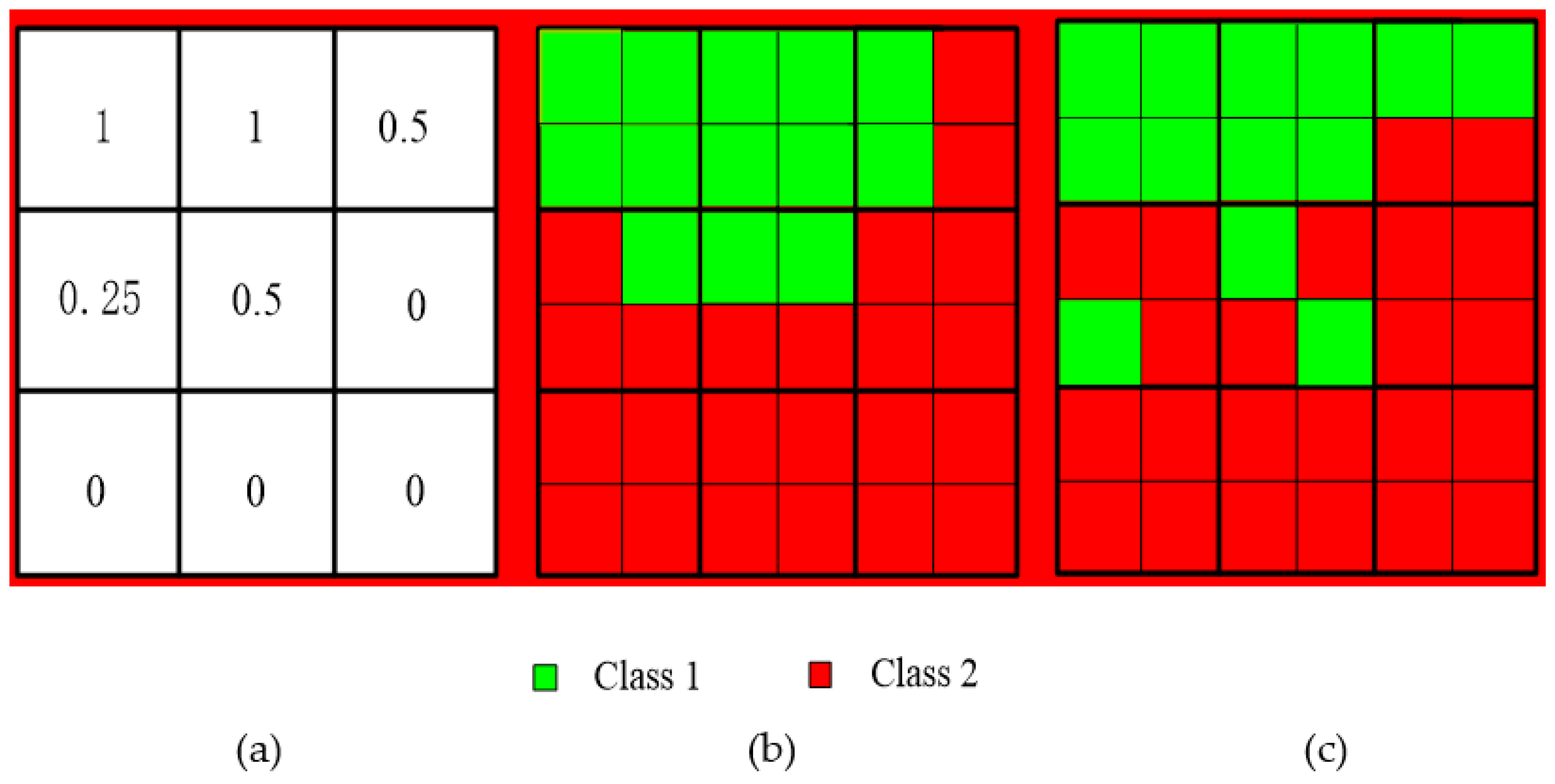
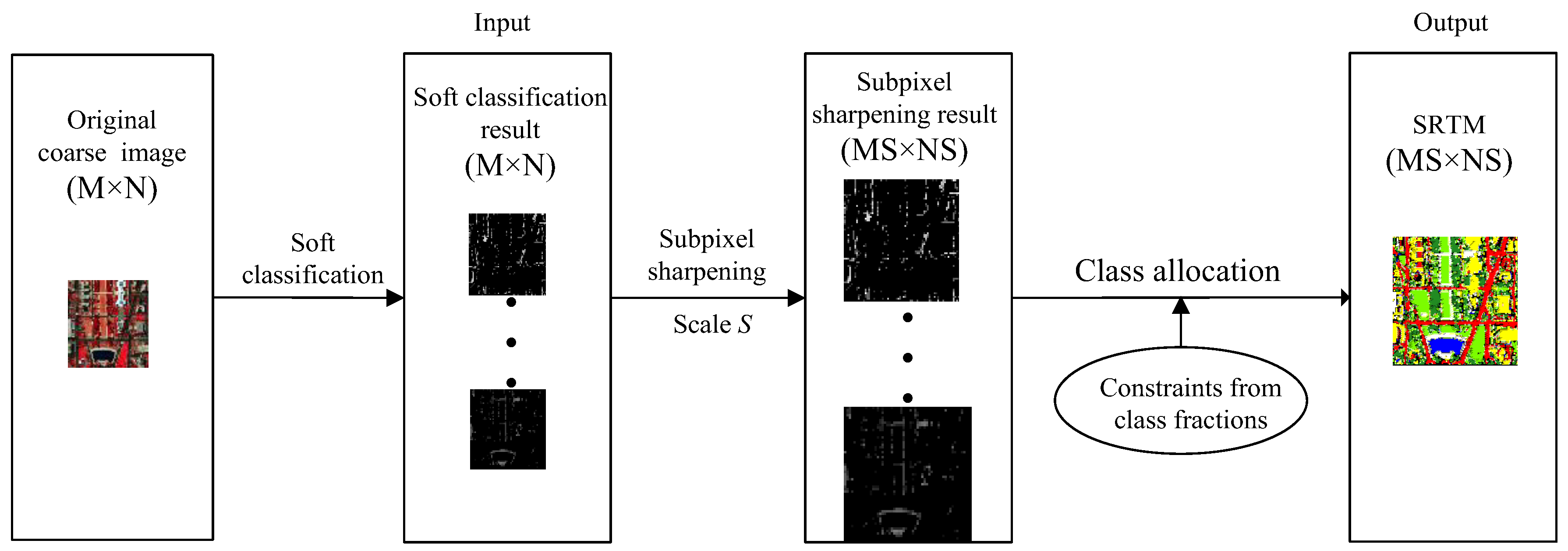
2. Soft-then-Hard Super-Resolution Mapping
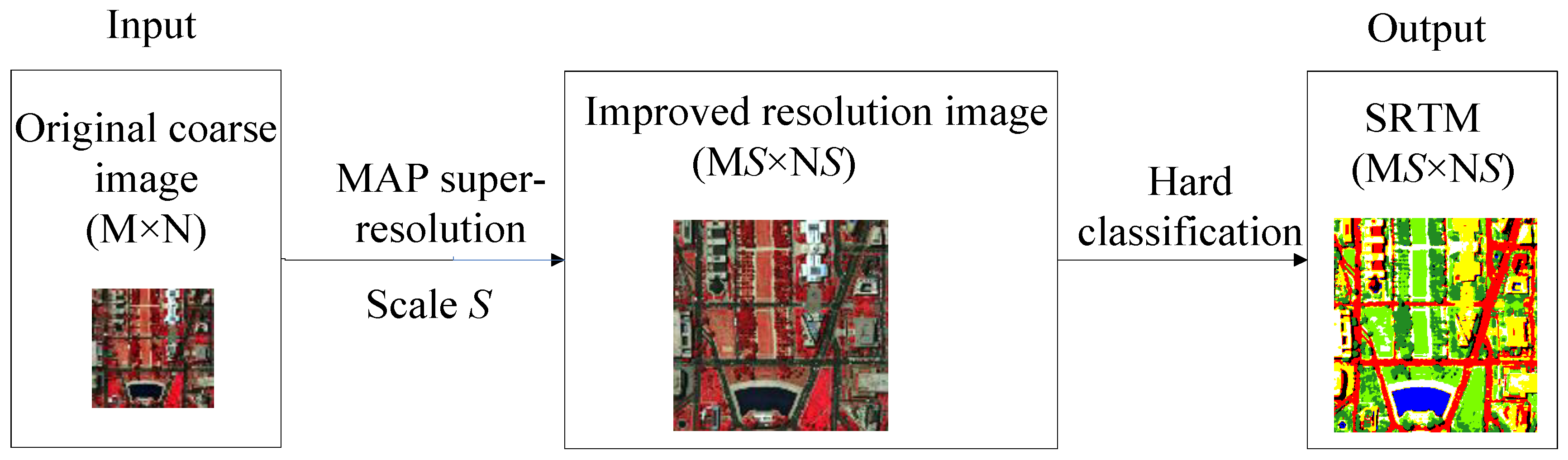
3. MAP Super-Resolution then Hard Classification
4. The Proposed Method
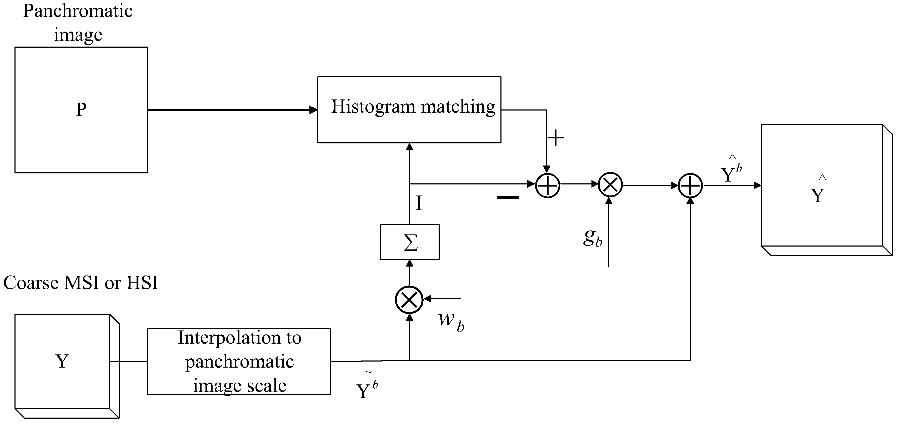
4.1. Pansharpening Technique
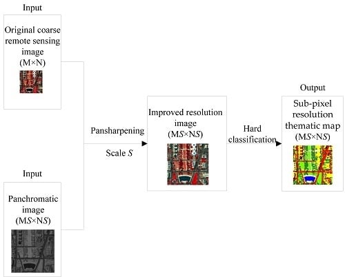
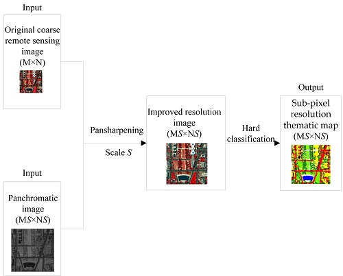
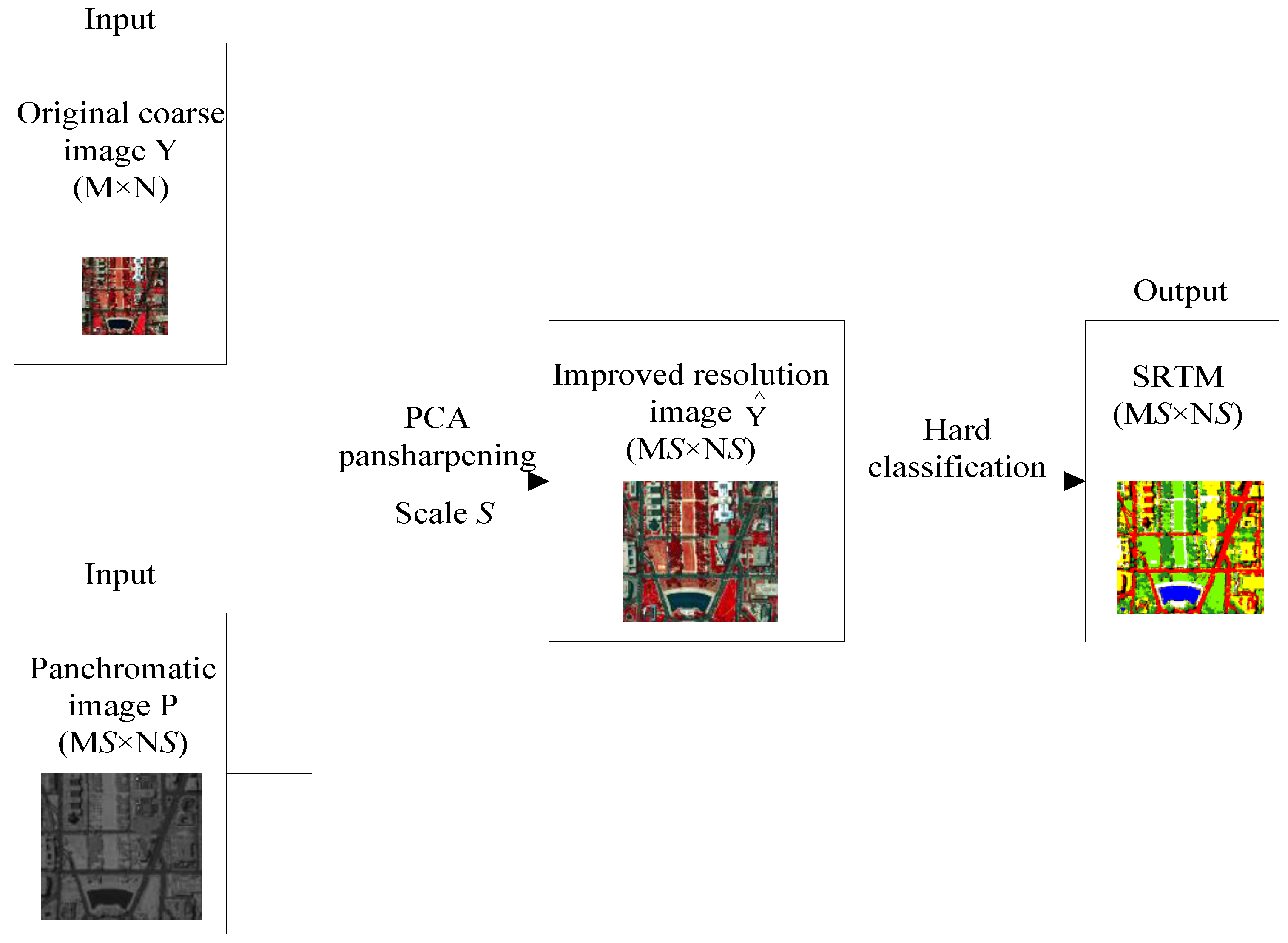
4.2. Pansharpening then Hard Classification
- Step (1)
- Utilizing the endmembers of interest (EOI) map the original high dimensional MSI or HSI into a low dimensional transformation space.
- Step (2)
- The original coarse MSI or HSI in the low dimensional transformation space and a panchromatic image are fused (see Equation (2)) with the PCA pansharpening technique, to generate an improved resolution image.
- Step (3)
- SRTM is produced by classifying the improved resolution image.
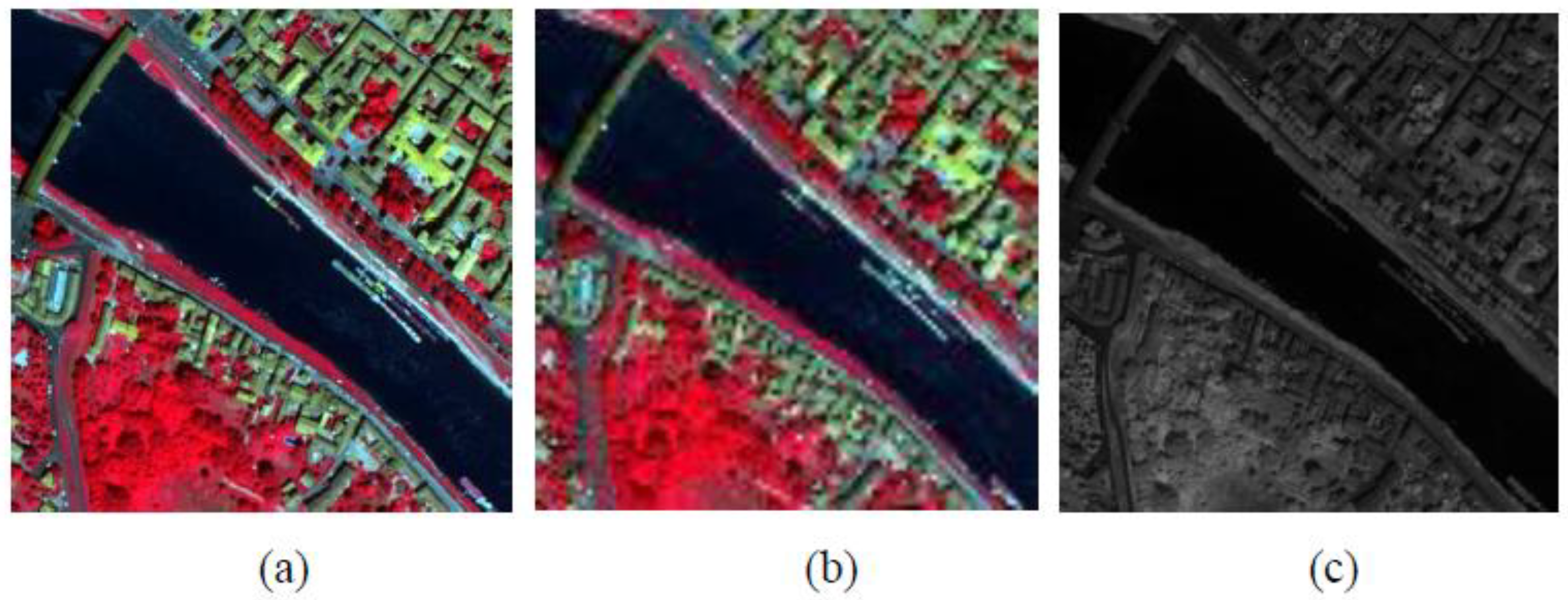
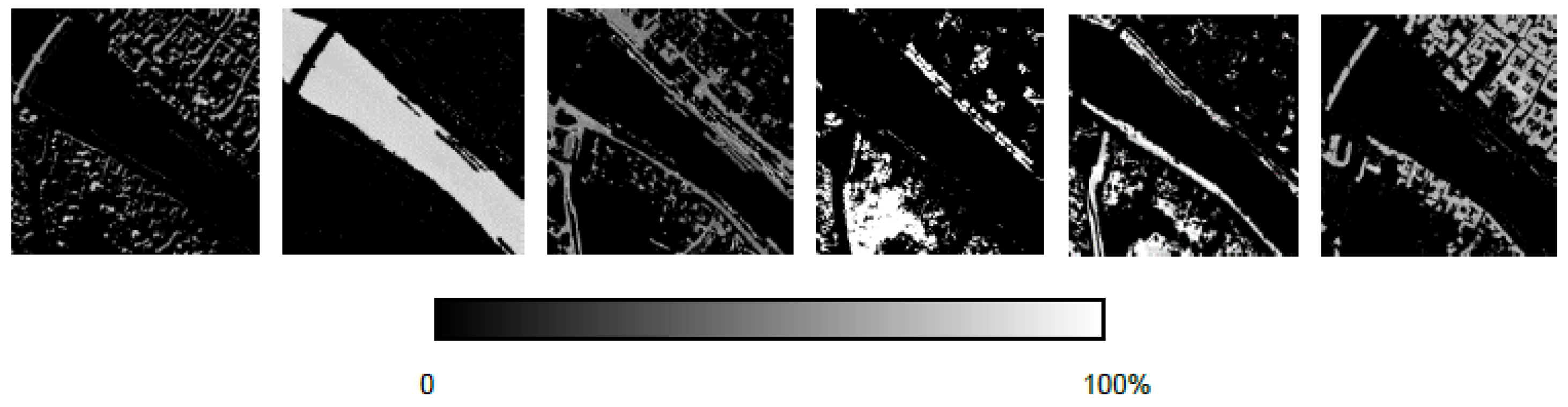
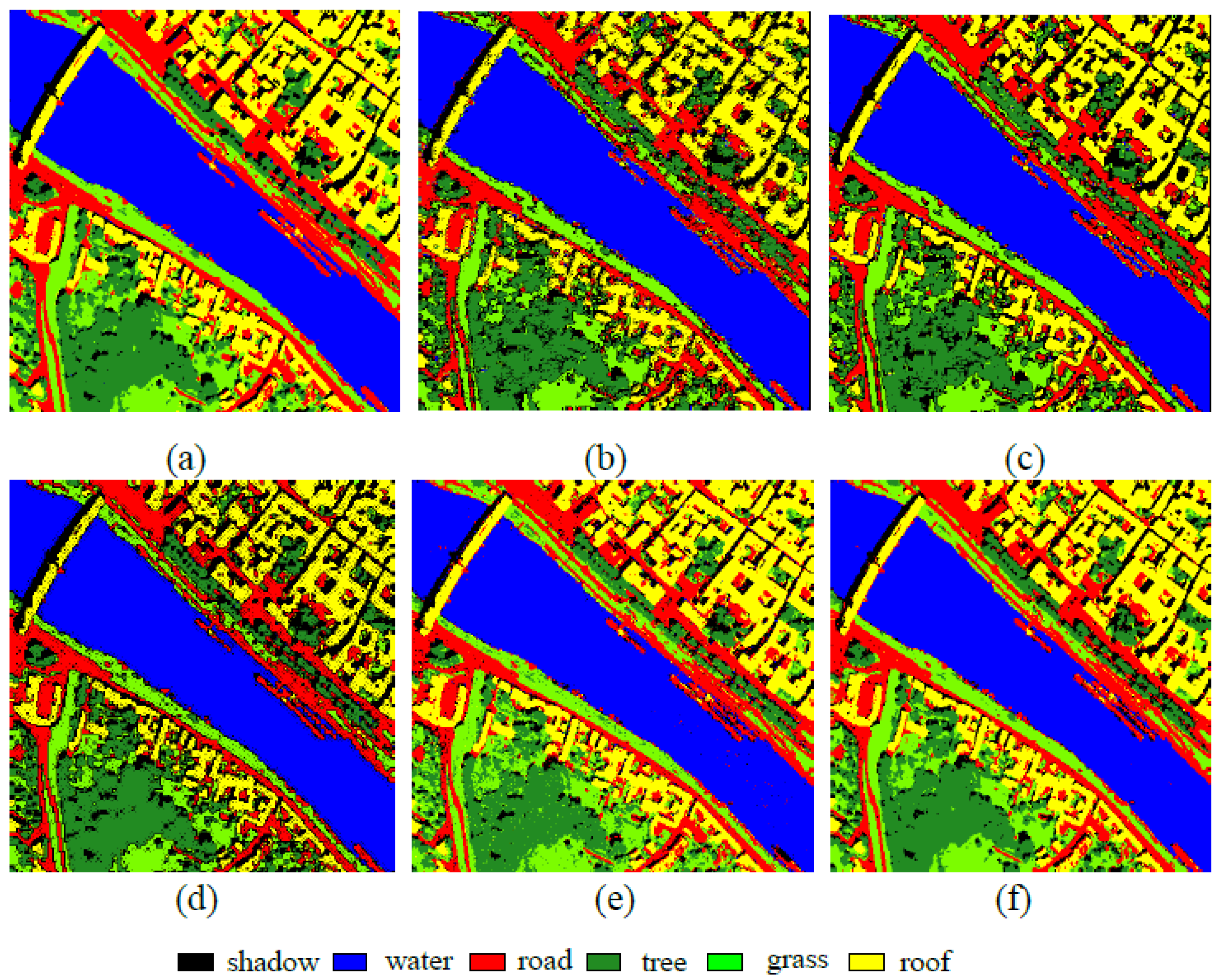
5. Experimental Analysis
5.1. Experiment 1
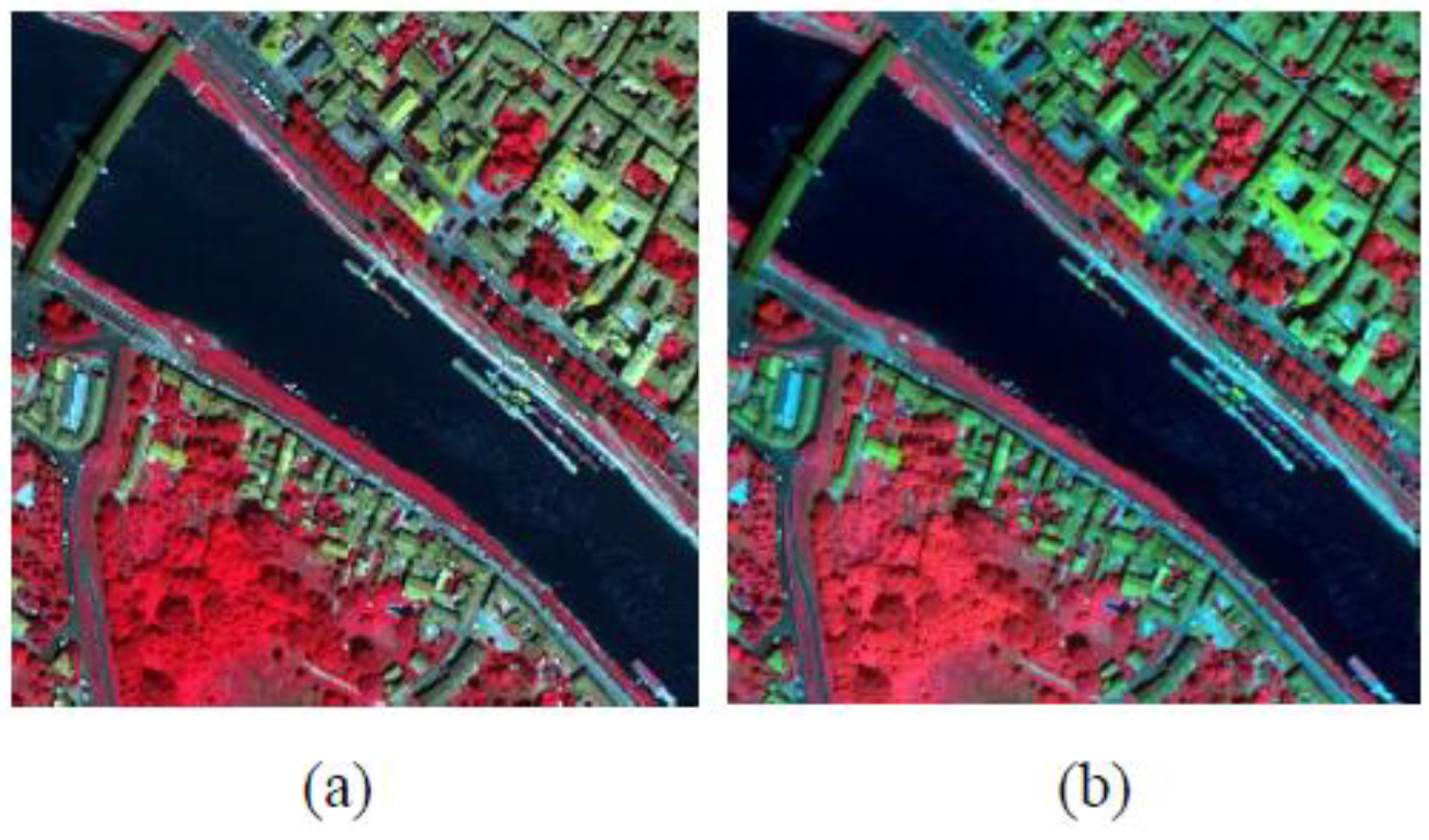
5.2. Experiment 2
6. Conclusions
Author Contributions
Acknowledgments
Conflicts of Interest
Abbreviation
| Acronyms | Acronym Definitions |
| MSI | Multispectral image |
| HSI | Hyperspectral image |
| SRM | Super-resolution mapping |
| STHSRM | Soft then hard super-resolution mapping |
| SRTM | Sub-pixel resolution thematic map |
| MAP | Maximum a posteriori probability |
| MTC | MAP super-resolution then hard classification |
| PTC | Pansharpening then hard classification |
| CS | Component substitution |
| PCA | Principal component analysis |
| LOT | Linear optimization technique |
| EOI | Endmembers of interest |
| COI | Classes of interest |
References
- Mura, M.D.; Prasad, S.; Pacifici, F.; Gamba, P.; Chanussot, J.; Benediktsson, J.A. Challenges and opportunities of multimodality and data fusion in remote sensing. Proc. IEEE 2015, 103, 1585–1601. [Google Scholar] [CrossRef]
- Villa, A.; Chanussot, J.; Benediktsson, J.A.; Jutten, C. Spectral unmixing for the classification of hyperspectral images at a finer spatial resolution. IEEE J. Sel. Top. Signal Process. 2011, 5, 521–535. [Google Scholar] [CrossRef]
- Wang, L.; Liu, D.; Wang, Q. Geometric method of fully constrained least squares linear spectral mixture analysis. IEEE Trans. Geosci. Remote Sens. 2013, 51, 3558–3566. [Google Scholar] [CrossRef]
- Halimi, A.; Altmann, Y.; Dobigeon, N.; Tourneret, J.Y. Nonlinear unmixing of hyperspectral images using a generalized bilinear model. IEEE Trans. Geosci. Remote Sens. 2011, 49, 4153–4162. [Google Scholar] [CrossRef]
- Wang, L.; Jia, X. Integration of soft and hard classification using extended support vector machine. IEEE Geosci. Remote Sens. Lett. 2009, 6, 543–547. [Google Scholar] [CrossRef]
- Wang, L.; Liu, D.; Wang, Q. Spectral unmixing model based on least squares support vector machine with unmixing residue constraints. IEEE Geosci. Remote Sens. Lett. 2013, 10, 1592–1596. [Google Scholar] [CrossRef]
- Bastin, L. Comparison of fuzzy c-means means classification, linear mixture modeling and MLC probabilities as tools for unmixing coarse pixels. Int. J. Remote Sens. 1997, 18, 3629–3648. [Google Scholar] [CrossRef]
- Schowengerdt, R.A. On the estimation of spatial-spectral mixing with classifier likelihood functions. Pattern Recognit. Lett. 1996, 17, 1379–1387. [Google Scholar] [CrossRef]
- Carpenter, G.M.; Gopal, S.; Macomber, S.; Martens, S.; Wooscock, C.E. A neural network method for mixture estimation for vegetation mapping. Remote Sens. Environ. 1999, 70, 138–152. [Google Scholar] [CrossRef]
- Atkinson, P.M. Mapping sub-pixel boundaries from remotely sensed images. In Innovations in GIS; Taylor & Francis: New York, NY, USA, 1997; pp. 166–180. [Google Scholar]
- Atkinson, P.M. Sub-pixel target mapping from soft-classified remotely sensed imagery. Photogramm. Eng. Remote Sens. 2005, 71, 839–846. [Google Scholar] [CrossRef]
- Niroumand-Jadidi, M.; Vitti, A. Reconstruction of river boundaries at sub-pixel resolution: Estimation and spatial allocation of water fractions. ISPRS Int. J. Geo-Inf. 2017, 6, 383. [Google Scholar] [CrossRef]
- Wetherley, E.B.; Roberts, D.A.; McFadden, J. Mapping spectrally similar urban materials at sub-pixel scales. Remote Sens. Environ. 2017, 195, 170–183. [Google Scholar] [CrossRef]
- Wang, Q.; Shi, W.; Wang, L. Allocating classes for soft-then-hard sub-pixel mapping algorithms in units of class. IEEE Trans. Geosci. Remote Sens. 2014, 5, 2940–2959. [Google Scholar] [CrossRef]
- Nigussie, D.; Zurita-Milla, R.; Clevers, J.G.P.W. Possibilities and limitations of artificial neural networks for subpixel mapping of land cover. Int. J. Remote Sens. 2011, 32, 7203–7226. [Google Scholar] [CrossRef]
- Shao, Y.; Lunetta, R.S. Sub-pixel mapping of tree canopy, impervious surfaces, and cropland in the Laurentian great lakes basin using MODIS time-series data. IEEE J. Sel. Top. Appl. Earth Obs. Remote Sens. 2011, 4, 336–347. [Google Scholar] [CrossRef]
- Tatem, A.J.; Lewis, H.G.; Atkinson, P.M.; Nixon, M.S. Super-resolution target identification form remotely sensed images using a Hopfield neural network. IEEE Trans. Geosci. Remote Sens. 2011, 39, 781–796. [Google Scholar] [CrossRef]
- Muad, A.M.; Foody, G.M. Impact of land cover patch size on the accuracy of patch area representation in HNN-based super resolution mapping. IEEE J. Sel. Top. Appl. Earth Obs. Remote Sens. 2012, 5, 1418–1427. [Google Scholar] [CrossRef]
- Mertens, K.C.; Basets, B.D.; Verbeke, L.P.C.; De Wulf, R. A sub-pixel mapping algorithm based on sub-pixel/pixel spatial attraction models. Int. J. Remote Sens. 2006, 27, 3293–3310. [Google Scholar] [CrossRef]
- Wang, P.; Wang, L. Soft-then-hard super-resolution mapping based on a spatial attraction model with multiscale sub-pixel shifted images. Int. J. Remote Sens. 2017, 38, 4303–4326. [Google Scholar] [CrossRef]
- Verhoeye, J.; De Wulf, R. Land-cover mapping at sub-pixel scales using linear optimization techniques. Remote Sens. Environ. 2002, 79, 96–104. [Google Scholar] [CrossRef]
- Jin, H.; Mountrakis, G.; Li, P. A super-resolution mapping method using local indicator variograms. Int. J. Remote Sens. 2012, 33, 7747–7773. [Google Scholar] [CrossRef]
- Wang, Q.; Atkinson, P.M.; Shi, W. Indicator cokriging-based subpixel mapping without prior spatial structure information. IEEE Trans. Geosci. Remote Sens. 2015, 53, 309–323. [Google Scholar] [CrossRef]
- Zhong, Y.; Wu, Y.; Xu, X.; Zhang, L. An adaptive subpixel mapping method based on MAP model and class determination strategy for hyperspectral remote sensing imagery. IEEE Trans. Geosci. Remote Sens. 2015, 53, 1411–1426. [Google Scholar] [CrossRef]
- Wang, Q.; Shi, W.; Atkinson, P.M. Sub-pixel mapping of remote sensing images based on radial basis function interpolation. ISPRS J. Photogramm. 2014, 92, 1–15. [Google Scholar] [CrossRef]
- Ling, F.; Du, Y.; Li, X.; Li, W.; Xiao, F.; Zhang, Y. Interpolation-based super-resolution land cover mapping. Remote Sens. Lett. 2013, 4, 629–638. [Google Scholar] [CrossRef]
- Wang, Q.; Shi, W. Utilizing multiple subpixel shifted images in subpixel mapping with image interpolation. IEEE Geosci. Remote Sens. Lett. 2014, 11, 798–802. [Google Scholar] [CrossRef]
- Wang, P.; Wang, L.; Chanussot, J. Soft-then-hard subpixel land cover mapping based on spatial-spectral interpolation. IEEE Geosci. Remote Sens. Lett. 2016, 13, 1851–1854. [Google Scholar] [CrossRef]
- Wang, P.; Wang, L.; Mura, M.D.; Chanussot, J. Using multiple subpixel shifted images with spatial-spectral information in soft-then-hard subpixel mapping. IEEE J. Sel. Top. Appl. Earth Obs. Remote Sens. 2017, 13, 1851–1854. [Google Scholar] [CrossRef]
- Jia, S.; Qian, Y. Spectral and spatial complexity-based hyperspectral unmixing. IEEE Trans. Geosci. Remote Sens. 2007, 45, 3867–3879. [Google Scholar]
- Chen, Y.; Ge, Y.; Heuvelink, G.B.M.; Hu, J.; Jiang, Y. Hybrid constraints of pure and mixed pixels for soft-then-hard super-resolution mapping with multiple shifted images. IEEE J. Sel. Top. Appl. Earth Obs. Remote Sens. 2015, 8, 2040–2052. [Google Scholar] [CrossRef]
- Ge, Y.; Chen, Y.; Stein, A.; Li, S.; Hu, J. Enhanced sub-pixel mapping with spatial distribution patterns of geographical objects. IEEE Trans. Geosci. Remote Sens. 2016, 54, 2356–2370. [Google Scholar] [CrossRef]
- Wang, L.; Wang, P.; Zhao, C. Producing Subpixel Resolution Thematic Map From Coarse Imagery: MAP Algorithm-Based Super-Resolution Recovery. IEEE J. Sel. Top. Appl. Earth Obs. Remote Sens. 2016, 9, 2290–2304. [Google Scholar] [CrossRef]
- Chang, C.; Wu, C.; Tsai, C. Random N-Finder (N-FINDR) Endmember Extraction Algorithms for Hyperspectral Imagery. Fast implementation of maximum simplex volume based endmember extraction in original hyperspectral data space. IEEE Trans. Geosci. Remote Sens. 2011, 20, 641–656. [Google Scholar]
- Vivone, G.; Alparone, L.; Chanussot, J.; Mura, M.D.; Garzelli, A.; Licciardi, G.; Restaino, R.; Wald, L. A critical comparison among pansharpening algorithms. IEEE Trans. Geosci. Remote Sens. 2015, 53, 2565–2585. [Google Scholar] [CrossRef]
- Loncan, L.; de Almeida, L.B.; Bioucas-Dias, J.M.; Briottet, X.; Chanussot, J.; Dobigeon, N.; Fabre, S.; Liao, W.; Licciardi, G.A.; Simoes, M.; et al. Hyperspectral pansharpening: A review. IEEE Geosci. Remote Sens. Mag. 2015, 3, 27–46. [Google Scholar] [CrossRef]
- Thomas, C.; Ranchin, T.; Wald, L.; Chanussot, J. Synthesis of multispectral images to high spatial resolution: A critical review of fusion methods based on remote sensing physics. IEEE Trans. Geosci. Remote Sens. 2008, 46, 1301–1312. [Google Scholar] [CrossRef]
- Aiazzi, B.; Baronti, S.; Selva, M. Improving component substitution pansharpening through multivariate regression of MS+Pan data. IEEE Trans. Geosci. Remote Sens. 2007, 45, 3230–3239. [Google Scholar] [CrossRef]
- Wang, L.; Hao, S.; Wang, Y.; Lin, Y.; Wang, Q. Spatial-spectral information-based semi-supervised classification algorithm for hyperspectral imagery. IEEE J. Sel. Top. Appl. Earth Obs. Remote Sens. 2014, 7, 3577–3585. [Google Scholar] [CrossRef]
- Chavez, P.S., Jr.; Sides, S.C.; Anderson, J.A. Comparison of three different methods to merge multiresolution and multispectral data: Landsat TM and SPOT panchromatic. Photogramm. Eng. Remote Sens. 1991, 57, 295–303. [Google Scholar]
- Tu, T.M.; Huang, P.S.; Hung, C.L.; Chang, C.P. A fast intensity-hue-saturation fusion technique with spectral adjustment for IKONOS imagery. IEEE Geosci. Remote Sens. Lett. 2004, 1, 309–312. [Google Scholar] [CrossRef]
- Zhang, L.; Zhang, L.; Tao, D.; Huang, X. Tensor discriminative locality alignment for hyperspectral image spectral-spatial feature extraction. IEEE Trans. Geosci. Remote Sens. 2013, 51, 242–256. [Google Scholar] [CrossRef]


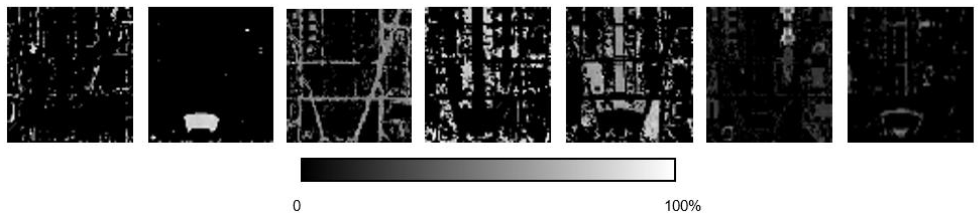
| MAP Result | Pansharpening Result | |
|---|---|---|
| Class 1 | 3.27% | 2.66% |
| Class 2 | 4.18% | 3.50% |
| Class 3 | 2.58% | 1.81% |
| Class 4 | 2.96% | 2.14% |
| Class 5 | 2.31% | 1.47% |
| Class 6 | 1.27% | 0.82% |
| Class 7 | 1.46% | 0.51% |
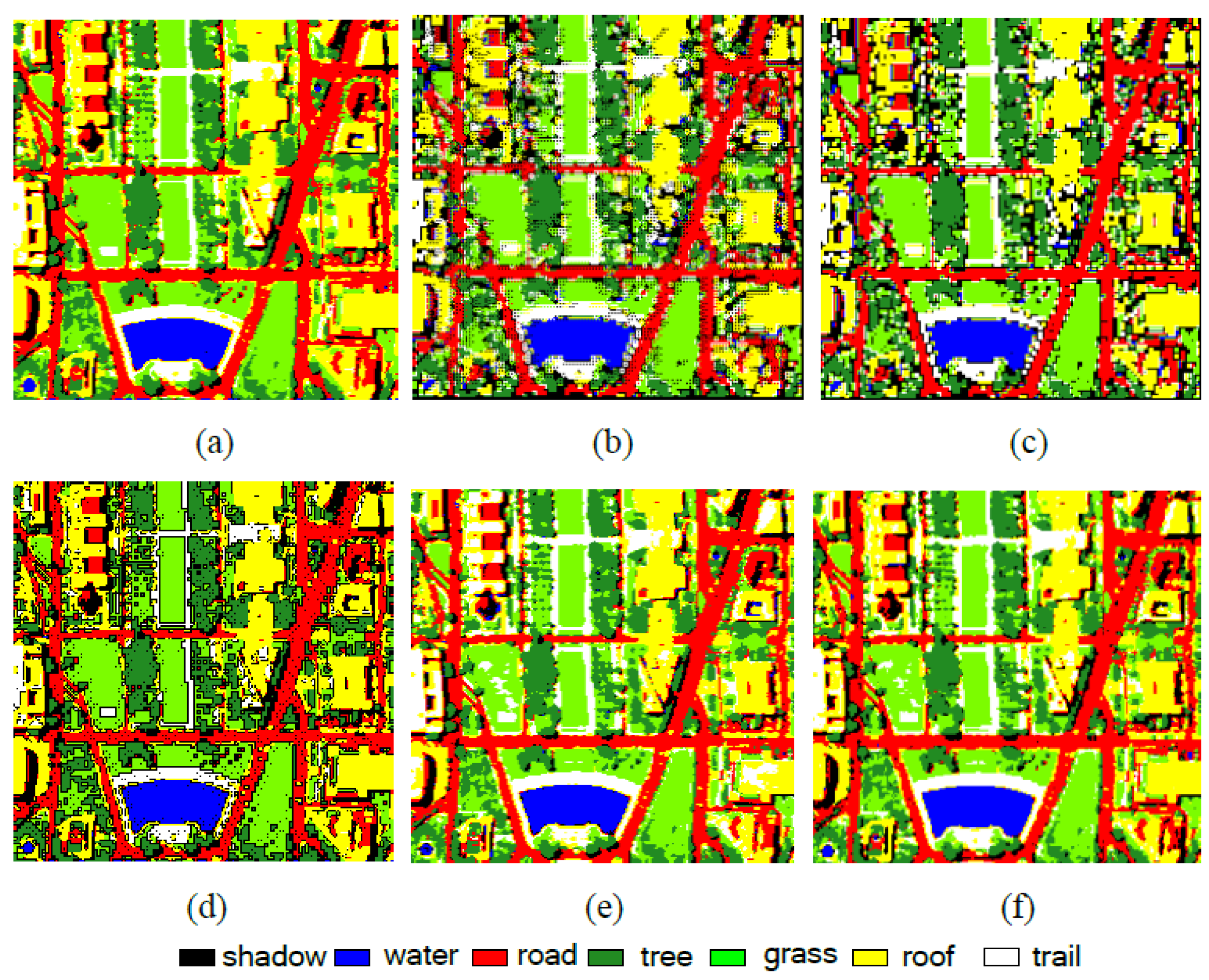
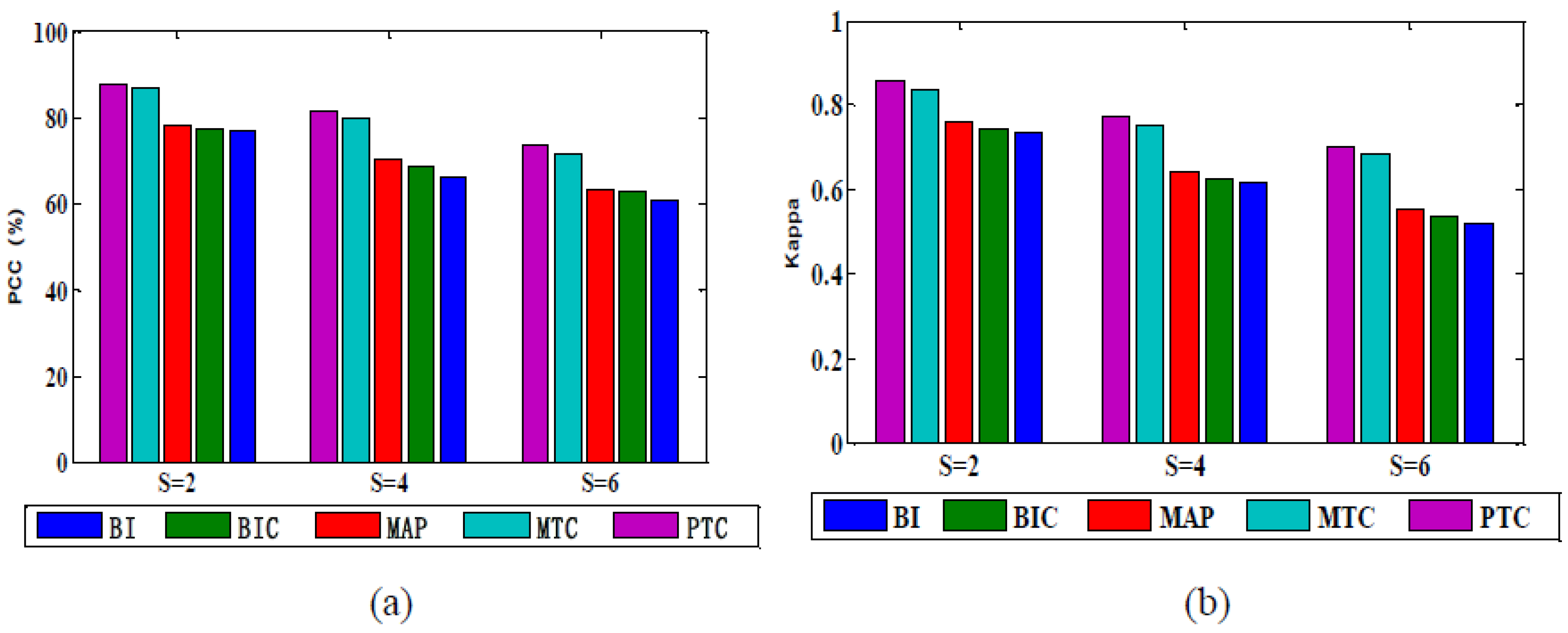
| BI | BIC | MAP | MTC | PTC | |
|---|---|---|---|---|---|
| Shadow | 73.44 | 75.03 | 77.50 | 78.77 | 80.13 |
| Water | 85.56 | 88.97 | 90.49 | 95.15 | 95.54 |
| Road | 70.55 | 72.74 | 75.73 | 88.75 | 90.31 |
| Tree | 72.45 | 75.45 | 77.36 | 97.47 | 98.04 |
| Grass | 74.70 | 78.60 | 82.19 | 88.86 | 89.51 |
| Roof | 70.67 | 72.98 | 75.09 | 85.23 | 88.43 |
| Trail | 73.88 | 75.58 | 77.98 | 87.16 | 90.35 |
| AA | 74.46 | 77.05 | 79.48 | 88.77 | 90.33 |
| PCC | 76.82 | 77.47 | 78.06 | 88.51 | 89.62 |
| BI | BIC | MAP | MTC | PTC | |
|---|---|---|---|---|---|
| Shadow | 77.59 | 82.36 | 82.94 | 84.28 | 86.13 |
| Water | 95.84 | 96.29 | 95.77 | 97.81 | 98.54 |
| Road | 71.69 | 74.51 | 73.23 | 93.36 | 95.31 |
| Tree | 74.28 | 75.63 | 77.36 | 94.68 | 97.04 |
| Grass | 69.23 | 71.40 | 71.71 | 90.34 | 92.51 |
| Roof | 79.75 | 82.07 | 80.81 | 97.69 | 98.43 |
| AA | 78.06 | 80.37 | 80.38 | 93.02 | 94.66 |
| PCC | 80.45 | 82.40 | 82.64 | 94.48 | 95.92 |
© 2018 by the authors. Licensee MDPI, Basel, Switzerland. This article is an open access article distributed under the terms and conditions of the Creative Commons Attribution (CC BY) license (http://creativecommons.org/licenses/by/4.0/).
Share and Cite
Wang, P.; Wang, L.; Wu, Y.; Leung, H. Utilizing Pansharpening Technique to Produce Sub-Pixel Resolution Thematic Map from Coarse Remote Sensing Image. Remote Sens. 2018, 10, 884. https://doi.org/10.3390/rs10060884
Wang P, Wang L, Wu Y, Leung H. Utilizing Pansharpening Technique to Produce Sub-Pixel Resolution Thematic Map from Coarse Remote Sensing Image. Remote Sensing. 2018; 10(6):884. https://doi.org/10.3390/rs10060884
Chicago/Turabian StyleWang, Peng, Liguo Wang, Yiquan Wu, and Henry Leung. 2018. "Utilizing Pansharpening Technique to Produce Sub-Pixel Resolution Thematic Map from Coarse Remote Sensing Image" Remote Sensing 10, no. 6: 884. https://doi.org/10.3390/rs10060884
APA StyleWang, P., Wang, L., Wu, Y., & Leung, H. (2018). Utilizing Pansharpening Technique to Produce Sub-Pixel Resolution Thematic Map from Coarse Remote Sensing Image. Remote Sensing, 10(6), 884. https://doi.org/10.3390/rs10060884