Abstract
Riparian forest (CP22) buffers are implemented in the Chesapeake Bay Watershed to trap pollutants in surface runoff thus minimizing the amount of pollutants entering the stream network. For these buffers to function effectively, overland flow must enter the riparian zones as dispersed sheet flow to facilitate slowing, filtering, and infiltrating of surface runoff. The occurrence of concentrated flowpaths, however, is prevalent across the watershed. Concentrated flowpaths limit buffer filtration capacity by channeling overland flow through or around buffers. In this study, two topographic metrics (topographic openness and flow accumulation) were used to evaluate the occurrence of concentrated flowpaths and to derive effective CP22 contributing areas in four Long-Term Agroecosystem Research (LTAR) watersheds within the Chesapeake Bay Watershed. The study watersheds include the Tuckahoe Creek watershed (TCW) located in Maryland, and the Spring Creek (SCW), Conewago Creek (CCW) and Mahantango Creek (MCW) watersheds located in Pennsylvania. Topographic openness identified detailed topographic variation and critical source areas in the lower relief areas while flow accumulation was better at identifying concentrated flowpaths in higher relief areas. Results also indicated that concentrated flowpaths are prevalent across all four watersheds, reducing CP22 effective contributing areas by 78% in the TCW, 54% in the SCW, 38% in the CCW and 22% in the MCW. Thus, to improve surface water quality within the Chesapeake Bay Watershed, the implementation of riparian forest buffers should be done in such a way as to mitigate the effects of concentrated flowpaths that continue to short-circuit these buffers.
1. Introduction
According to the United States Environmental Protection Agency (EPA) “dirty waters” list, Chesapeake Bay is one of the most polluted water bodies in the United States. The Chesapeake Bay Watershed has been widely studied, with many researchers concluding that the decline in water quality in Chesapeake Bay is largely attributed to an overabundance of sediment, nitrogen and phosphorus in surface runoff, particularly from agricultural lands [1,2,3,4,5,6,7].
In 2010, the EPA established a Total Maximum Daily Load (TMDL) for the Chesapeake Bay Watershed to ensure that all pollution control measures needed to fully restore the Bay’s water quality are in place by 2025, with practices in place by 2017 to meet 60 percent of the overall sediment, nitrogen and phosphorus reductions. Riparian forest (CP22) buffers are a substantial component of the best management practices promoted under the TMDL. CP22 buffers are a relatively established and accepted conservation practice used to protect water quality and enhance aquatic and wildlife habitats. These buffers typically comprise trees, shrubs, grasses and forbs planted along a stream or river. They are intended to intercept surface runoff, trap sediment, and subsequently reduce nitrogen and phosphorus loadings in the stream [8,9,10]. The vegetation in riparian zones helps to remove excess nutrients from lateral subsurface flow [11,12]. Riparian zones often consist of organic-rich soils that promote biological activity, resulting in macropores that act as preferential flowpaths through the soil, which increase infiltration and exfiltration [13,14].
Under the Conservation Reserve Program (CRP) and the Conservation Reserve Enhancement Program (CREP), farmers and land owners are incentivized to implement conservation practices such as CP22 buffers [15] on environmentally sensitive land. USDA agencies (Farm Service Agency, Agricultural Research Service and Forest Service) and Penn State University have recently joined forces in an extensive assessment of CP22 buffers and their contribution within the Chesapeake Bay Watershed.
Riparian buffers are most effective when surface runoff enters the riparian zone as dispersed sheet flow. In other words, riparian buffers function best under divergent flow conditions [9,16,17,18,19,20]. Under convergent flow conditions, where surface runoff occurs in concentrated flowpaths, the riparian buffers’ effectiveness is reduced. Concentrated flowpaths are hydrologic bypass features that concentrate overland flow through or around buffers and reduce the effective buffers’ filtering functions, thus rendering them less effective for sediment, nitrogen and phosphorus removal [16,21,22,23,24]. Persistence of concentrated flows may lead to the formation and erosion of hydrologic features such as rills and gullies. Typically, the trapping efficiencies of riparian buffers is the focus of studies investigating the effectiveness of riparian buffers [10,25,26]. Although sediment trapping efficiency is typically greater than 70% [25,26], sediment trapping capacities and subsequent nutrient removal are site-specific and vegetation-specific [27,28].
In recent years, researchers have started paying more attention to concentrated flowpaths through riparian buffers [17,24], however, few have focused on the identification of these concentrated flowpaths and how they affect the overall surface runoff-contributing areas to the buffers. This is partly due to a lack of high resolution digital elevation models (DEMs) and quantitative methods for evaluating surface runoff patterns. A study conducted on four farms in southeastern Nebraska [16] demonstrated that the concentration of runoff flow is common and substantially reduces the ability of riparian buffers to trap sediment (by as much as 78%). A similar study in the Spring Creek watershed, Pennsylvania, found that existing forest buffers intercepted runoff from only 23% of the potential drainage area due to the presence of concentrated flowpaths that developed [29].
This study (1) examined two methods for evaluating concentrated flowpaths in riparian buffer contributing areas, and (2) used the most appropriate method to demonstrate the impact of concentrated flowpaths on reducing the effective contributing area of riparian forest buffers. The results of this study provided insight into areas of improvement within existing buffer practice standards.
2. Materials and Methods
2.1. Study Area Description
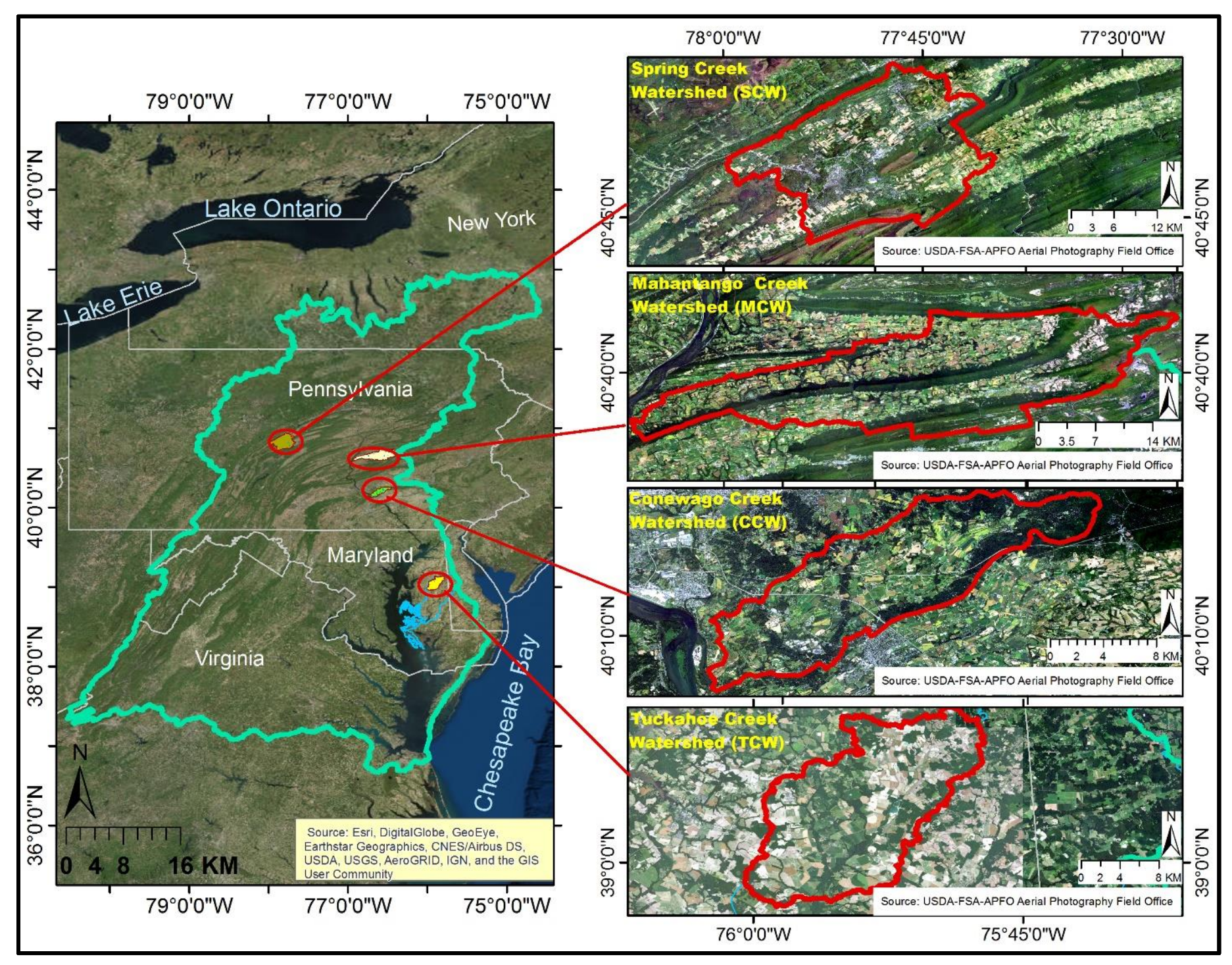
All study watersheds are within the Chesapeake Bay Watershed. The Chesapeake Bay Watershed is a 165,760 km2 catchment encompassing parts of six states (Delaware, Maryland, New York, Pennsylvania, Virginia and West Virginia) and the entire District of Columbia. Four Long-Term Agroecosystem Research (LTAR) watersheds (Tuckahoe Creek, Conewago Creek, Mahantango Creek and Spring Creek) were selected for this study because they represent a diversity of physiographic conditions, diversified agricultural production systems and a predominance of small farms with at least one CP22 contract. The watersheds under study were initiated under the USDA NRCS Conservation Effects Assessment Project (CEAP) to quantify the environmental effects of conservation practices. CEAP was initiated in 2003 to quantify the environmental benefits of conservation practices and to provide a measure of accountability for the millions of dollars being spent on conservation programs [30,31]. These watersheds were adopted by the USDA LTAR network which was established in 2011 [32].
The Tuckahoe Creek watershed (TCW) is approximately 371 km2 and is in the headwaters of the Choptank River basin in the Coastal Plains of the Chesapeake Bay Watershed (Figure 1). Major land uses are agriculture (54.0%) and forestry (33%). The average annual precipitation and temperature in TCW is 1120 mm and 13.3 °C, respectively. Most soils in the watershed are composed of Pocomoke-Fallsington-Sassafras association, which are poorly-drained, hydric soils [33]. TCW has low topographic relief (<30 m elevation), with a drainage pattern similar to a lagoonal drainage pattern [34]. Due to the flat topography and poorly-drained soils, farmers have historically utilized a network of drainage ditches to facilitate the movement of water to the stream network. Poor water quality in the TCW due to excess sedimentation has resulted in the degradation of its instream biological community. There are 13 (currently enrolled) riparian forest buffers with ages ranging from five to 15 years old implemented in the TCW to help mitigate water quality concerns. The main species of trees and shrubs that make up the CP22 buffers include sweetgum, hawthorn, black cherry, red maple, black walnut, black locust, and loblolly pine. More information on the Choptank River basin and TCW is presented in [35].
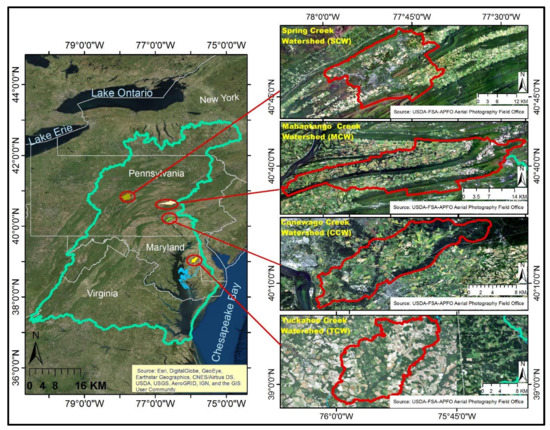
Figure 1.
Location of the study watersheds relative to the Chesapeake Bay Watershed: Spring Creek (SCW), Mahantango Creek (MCW), Conewago Creek (CCW) and Tuckahoe Creek (TCW) watersheds.
Runoff from the Conewago Creek (CCW = 136 km2), Mahantango Creek (MCW = 420 km2) and Spring Creek (SCW = 378 km2) watersheds drains to the Susquehanna river, the largest river in the Chesapeake Bay Watershed. All three watersheds are dominated by agriculture (36% in CCW, 44% in MCW and 28% in SCW) and forest (47% in CCW, 55% in MCW and 45% in SCW) [36]. Most soils in the CCW contain Lewisberry-Steinsburg and Penn associations. Lewisberry-Steinsburg soils are moderately deep, well drained soils formed on dissected ridges and low hills, and Penn soils are moderately deep soils that are well drained and formed on ridges and hills [33]. Most soils in the MCW are comprised of the Leck Kill-Meckesville-Calvin, Berks-Weikert-Bedington, and Hazleton-Dekalb-Buchanan series, which are moderately deep, well drained soils [33,36]. Most soils in the SCW are comprised of Hagerstown-Opequon-Hublerburg and Hazleton-Laidig-Andover series. Hagerstown-Opequon-Hublerburg soils are deep to shallow, well-drained soils. Hazleton-Laidig-Andover soils are gently sloping to very steep, deep, well drained and poorly drained soils [33].
The CCW is situated in the Gettysburg-Newark Lowland section of the Piedmont Physiographic Province, which consists mainly of rolling low hills and valleys [37]. The drainage pattern in the CCW is dendritic [37], with moderate to high topographic relief (>90 m elevation). The MCW is situated in the Susquehanna Lowland and Anthracite Upland sections of the Appalachian Ridge and Valley physiographic region. The Susquehanna Lowland section consists mainly of low to moderately high linear ridges and valleys, while the Anthracite Upland section consists mainly of narrow to wide irregular hills. The drainage pattern in the MCW is trellis and angulate in the Susquehanna Lowland section, with low to moderate topographic relief, and trellis and parallel in the Anthracite Upland section, with low to high topographic relief. The SCW is situated in the Appalachian Mountain section of the Ridge and Valley Physiographic Province, which consists mainly of long, narrow ridges and broad to narrow valleys. The drainage pattern in the SCW is trellis, angulate, and some karst, with moderate to very high topographic relief.
Excess nutrients and sediment in overland flow resulted in the degradation of surface water quality in the CCW, MCW and SCW watersheds. There are 13, 25 and three (currently enrolled) riparian forest buffers implemented in the CCW, MCW and SCW watersheds, respectively. Like those in TCW, the age of CP22 buffers in all three Pennsylvania watersheds range from five to 15 years old. In addition to improving water quality, fish and wildlife habitat, CP22 buffers may also be designed and implemented to provide opportunities for harvesting products such as nuts, berries and woody florals.
2.2. Data Description
The 3-m-DEMs used in this study were constructed by the USDA Agricultural Research Service (ARS) at Beltsville, Maryland from LiDAR elevation points taken across the Chesapeake Bay Watershed. Data points were collected using a Leica ALS50-II sensor with a scan angle of ±25° at a height of 1830 m above the Earth’s surface with a pulse rate of 126,000 Hz and scan frequency of 50 Hz [38]. As described in [38,39], raw data were converted to LAS files, containing x, y, z, and intensity data. Bare earth points were classified by the data provider using Terrascan and Fugro EarthData proprietary software (Fugro EarthData, Inc., Houston, TX, USA). A Trimble RTK 4700 GPS/base station combination and surveyed benchmarks were used to validate LiDAR data with over 100 precision GPS points collected at areas of stable elevation (e.g., road intersections). The resulted DEM had a vertical accuracy of ≤0.15 m and a pulse density of ~2.8 pts/m2 (~0.35 m post spacing) [38].
A buffer polygon layer consisting of all the active CREP buffers across the Chesapeake Bay Watershed was obtained from the USDA ARS. The buffer polygon layer was created by experts at the Natural Resources Conservation Agency (NRCS) as described in [40]. After obtaining the polygon layer, all CP22 buffer polygons were rectified with the stream network to ensure proper digitization. There were 14,391 CP22 buffers enrolled at the time of the study throughout the Chesapeake Bay Watershed, 9280 of these were within Maryland and Pennsylvania. Fifty-two CP22 buffers that are currently enrolled in the CREP project were selected from the four LTAR watersheds (11 in TCW, 13 in CCW, 25 in MCW and 3 in SCW) to evaluate the applicability of two topographic metrics in evaluating flow routing in CP22 buffer contributing areas.
Potential topographic contributing areas (TCAs) for each of the selected CP22 buffers were delineated from the LiDAR-derived DEM using the ArcGIS hydrology toolbox. These potential contributing areas were important in spatially reconciling the forest buffer polygons derived from an aerial photo and the grid-based stream network created by the 3-m DEM. In cases where sections of the stream network intersected the CP22 gridded polygons instead of running parallel to them, 5-m GIS masks were created around the stream reach and used to erase portions of the CP22 polygons. This enabled refinement of the “potential” contributing area to correctly identify only those grid cells contributing flow into the CP22 gridded polygons. Without this adjustment, some contributing areas would have erroneously been delineated for the entire stream reach, as illustrated in Figure 2. The DEMs masked by “potential” contributing area were then input into the System for Automated Geoscientific Analyses (SAGA) [41] to develop topographic metrics.
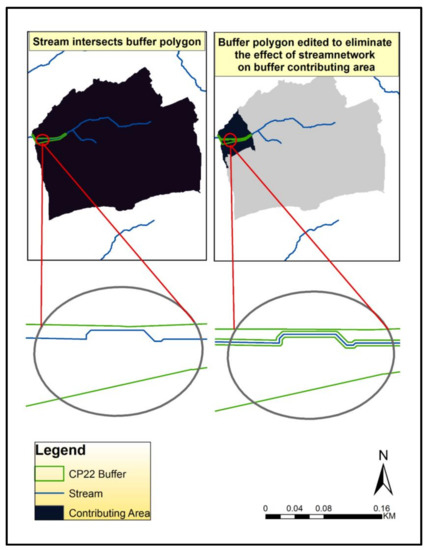
Figure 2.
Contributing area restricted to the riparian forest (CP22) buffer by erasing a portion of the CP22 buffer that is intersected by the stream network.
2.3. Topographic Analysis
Two topographic metrics (topographic openness and flow accumulation) were quantified from unfiltered 3-m LiDAR-derived DEMs [42] using SAGA version 3.0.0 (Institute of Geography, Hamburg, Germany), and used to assess concentrated flowpaths and hydrologic bypass features affecting 52 riparian forest (CP22) buffers. The vertical distances of DEMs used to generate the topographic openness maps for low relief areas were multiplied by 100 to increase distinguishability in relatively flat surfaces. The exaggerated DEMs were then smoothed twice through a low pass filter and used as the input for the SAGA Topographic Openness module to develop openness maps. Figure 3 shows a side-by-side comparison of the SAGA topographic openness and the LiDAR-derived DEM used as input to SAGA.
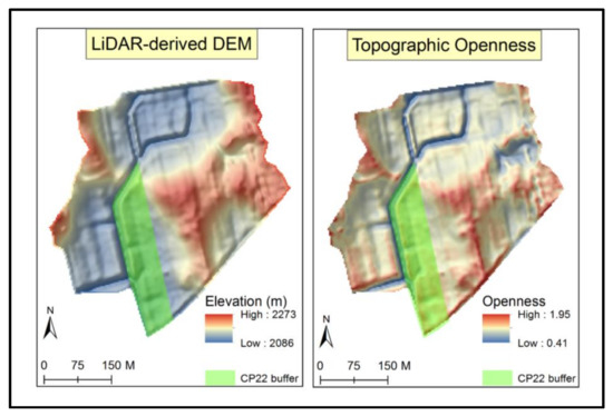
Figure 3.
A comparison of the LiDAR-derived digital elevation model (DEM) and the System for Automated Geoscientific Analyses (SAGA) Topographic Openness.
Topographic openness measures the angular relation between surface relief and horizontal distance, and is used to visualize topographic character by expressing the degree of dominance (positive) or enclosure (negative) of a landscape location [43]. In preliminary studies, it was easier to distinguish hydrologic features’ positive openness compared to negative openness. For this reason, positive openness was used to conduct the flowpath analyses in this study. Positive openness, , at a location on a surface within the radial distance, L, on the DEM, as shown in (1), is the average of zenith angles measured from a central point to the surface for all eight compass directions and the point yielding the highest angle viewed above the surface along each of the eight azimuths (0°, 45°, …, 315°) up to the specified radial distance L. The radial distance selected for this analysis was 10,000 floating points. A more detailed explanation of topographic openness is presented in [43].
Flow accumulation maps were created from the non-exaggerated 3-m DEM using the “top-down” approach in which a set of algorithms process a DEM downwards from the highest elevation to lowest elevation for calculation of flow accumulation. Flow accumulation measures the accumulated flow to each cell in a DEM. As the number of cells draining to a certain area increases, the more concentrated the flow in that area becomes. These areas of high flow accumulation may provide concentrated flows during storm events.
To generate flow accumulation layers, the DEMs were input into SAGA, and the D-Infinity flow directions algorithm applied [44]. Pits were not filled, because this step is generally undertaken to correct errors in existing DEMs, and the DEMs generated for this project were error-corrected prior to this step. By representing flow direction as a single angle taken at the steepest downward slope on the eight triangular facets centered at each grid point, the D-Infinity method marks an improvements over prior procedures that have restricted flow to just eight possible directions [44]. This approach minimizes the effects of grid artifacts on the determination of flow directions and specific catchment areas.
The maps generated for both topographic metrics were used to identify flow routing patterns within each TCA. The presence of hydrologic bypass features captured by the topographic openness and flow accumulation maps were confirmed in subsequent visits to the Choptank River and Conewago Creek watersheds.
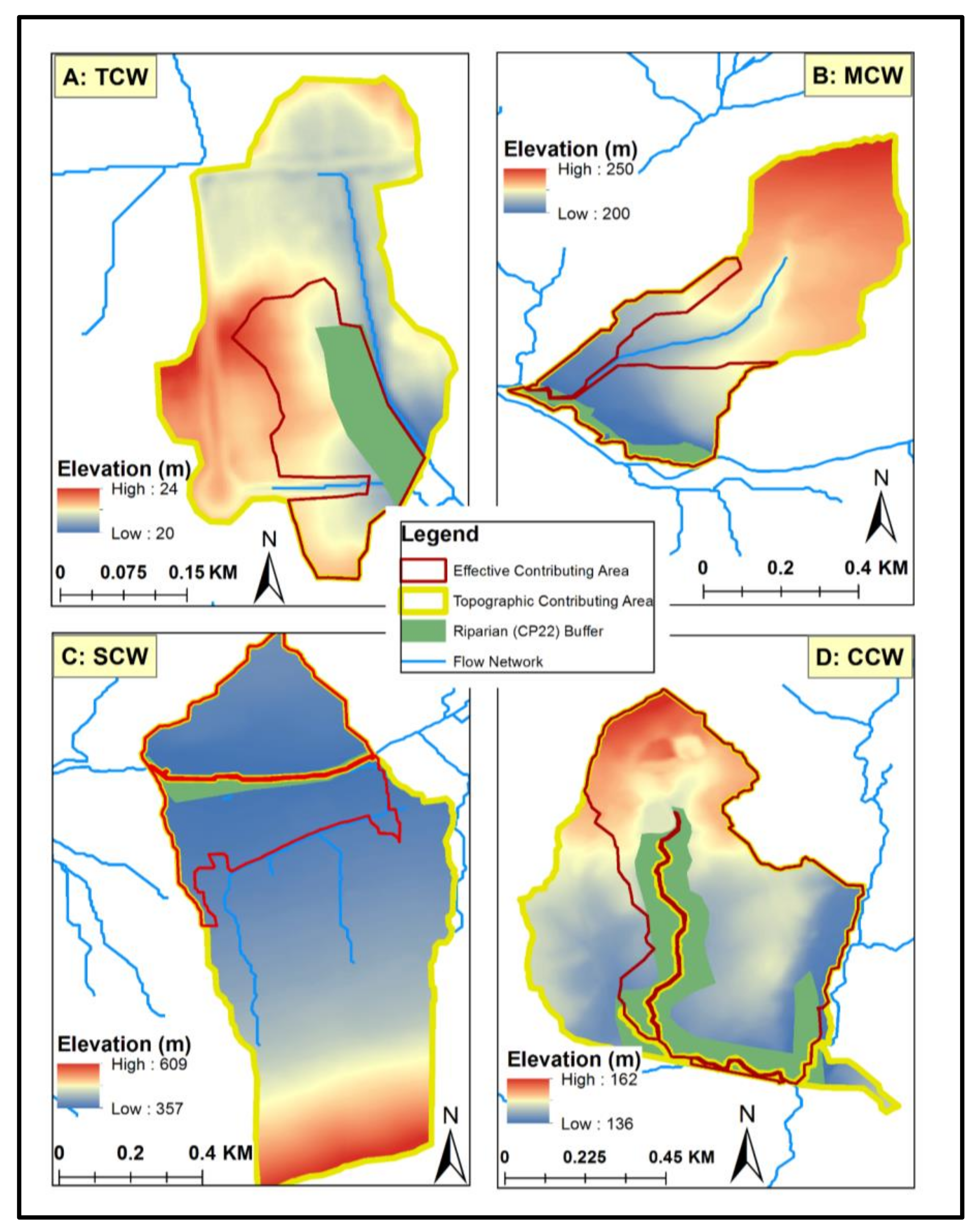
A stream threshold value of 5000 was judged to best capture the concentrated flowpaths into and through the buffers and was used to generate a final flow network. The final flow network was then used to assess the effective contributing area (ECA) for each of the CP22 buffers. Figure 4 illustrates the TCA and ECA of a riparian forest buffer in each of the four watersheds. ECA refers to the portion of TCA that contributes runoff to the forest buffers in the form of sheet flow. Therefore, the portion of the catchment area that conveys surface runoff directly to the stream channel via concentrated flow such that the runoff is minimally, if at all, filtered by the CP22 buffers, was determined to be the difference between TCA and ECA.

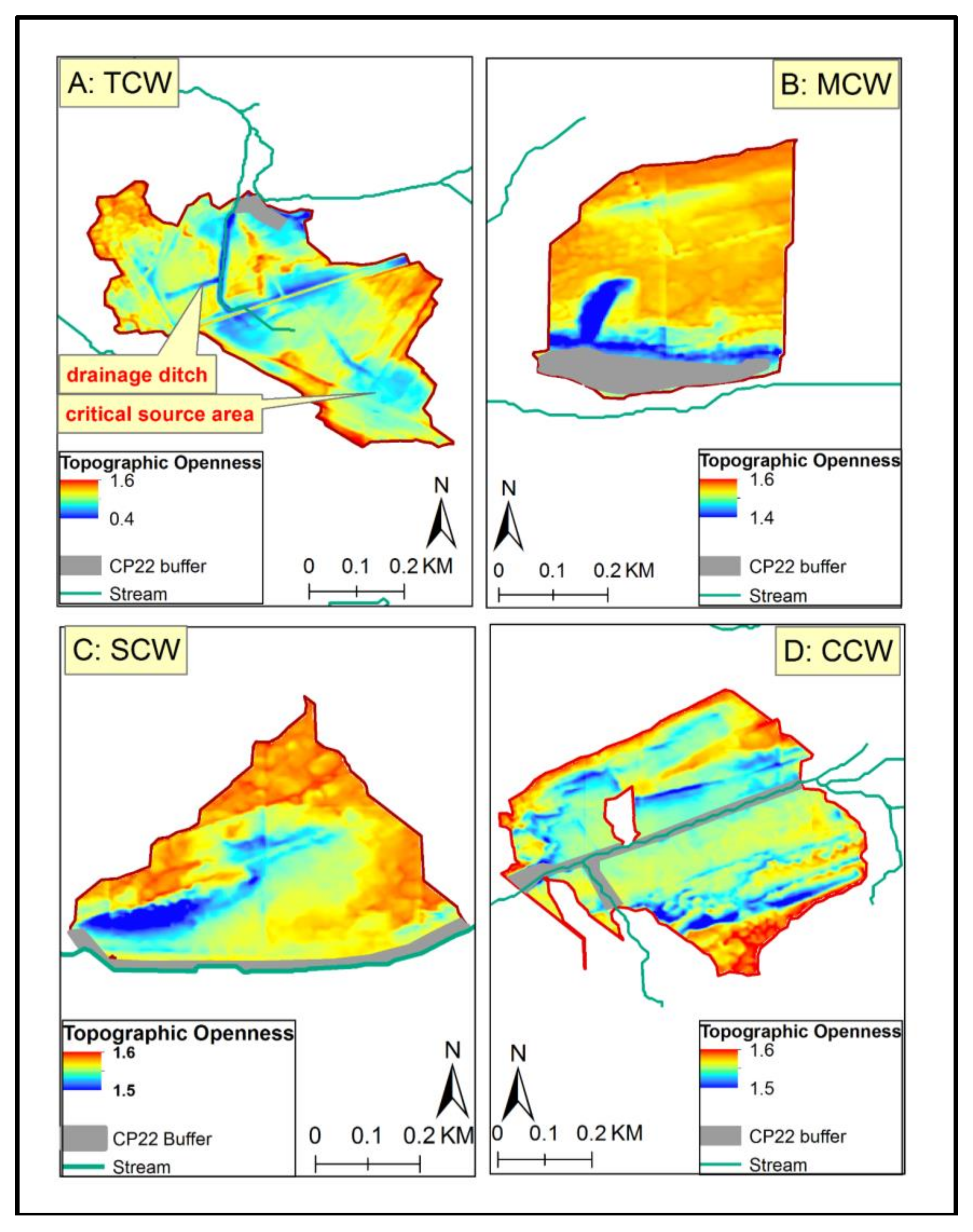
Figure 4.
Examples of potential topographic (TCA) and effective (ECA) contributing areas for riparian forest (CP22) buffers in TCW (A), MCW (B), SCW (C) and CCW (D) watersheds.
3. Results
3.1. A Comparison of Topographic Metrics
Topographic metrics such as topographic openness and flow accumulation have made it possible to visualize flow routing patterns at different topographic reliefs. The results presented here in the form of topographic maps highlight the strengths and limitations of both techniques.
The topographic openness shows detailed topographic variation in the lower relief TCW (Figure 5A) when compared to the higher relief areas of SCW, CCW, and MCW watersheds (Figure 5B–D). Figure 5A highlights critical source areas and the numerous ditches used to enhance overland flow. These ditches create features that transport surface runoff directly to the stream channel, bypassing the forest buffers without much chance for remediation. Openness images for CP22 buffer contributing areas in the Piedmont and the Ridge and Valley physiographic regions (Figure 5B–D.) showed major flow accumulation areas but not the detailed drainage pattern, berms and critical source areas within the respective contributing areas. This suggests the applicability of topographic openness may be limited to landscapes with lower relief (<30 m elevation change). Though beyond the scope of this study, it should be noted that vertical exaggeration of the DEMs improved the ability of topographic openness to display hydrologic features in low relief areas, but the opposite effect was true for the high relief areas.

Figure 5.
Map of topographic openness for riparian forest (CP22) buffers contributing areas in TCW (A), MCW (B), SCW (C) and CCW (D).
Figure 6 shows the flow accumulation maps for the forest buffer contributing areas presented in Figure 5. In contrast to the topographic openness, when the flow accumulation approach was used to map flow routing in low relief areas (Figure 6A), it resulted in a dense drainage network with many intersections. This made it difficult to visualize not only the direction of flow but also the flow connectivity. However, as shown in Figure 6B–D, it is much easier to visualize the direction of flow and the flow connectivity in higher relief areas. The areal extent of the critical source areas was also not visible with the flow accumulation maps, which could further limit the flow accumulation applicability in lower relief areas. Though it is assumed that areas that have a lot of concentrated flow and direct pathways to the stream are contributing pollutants that are in the critical source areas, it would be more difficult to implement measures that directly target critical source areas. With the flow accumulation maps, however, the presence of features (such as berms and swales) that obstruct overland flow in the higher relief areas were noticed more readily.
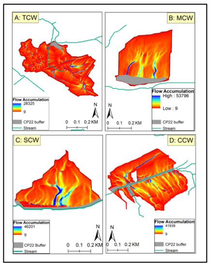
Figure 6.
Maps of flow accumulation for riparian forest (CP22) buffers contributing areas in TCW (A), MCW (B), SCW (C) and CCW (D).
3.2. Analysis of Hydrologic Bypass Features
Topographic openness and flow accumulation were used to assess the contributing areas to CP22 buffers. Table 1 summarizes the analysis of 52 riparian buffer contributing areas within four LTAR watersheds.

Table 1.
Summary of riparian buffer analysis in the Tuckahoe Creek (TCW), Spring Creek (SCW), Conewago Creek (CCW), and Mahantango Creek (MCW) watersheds.
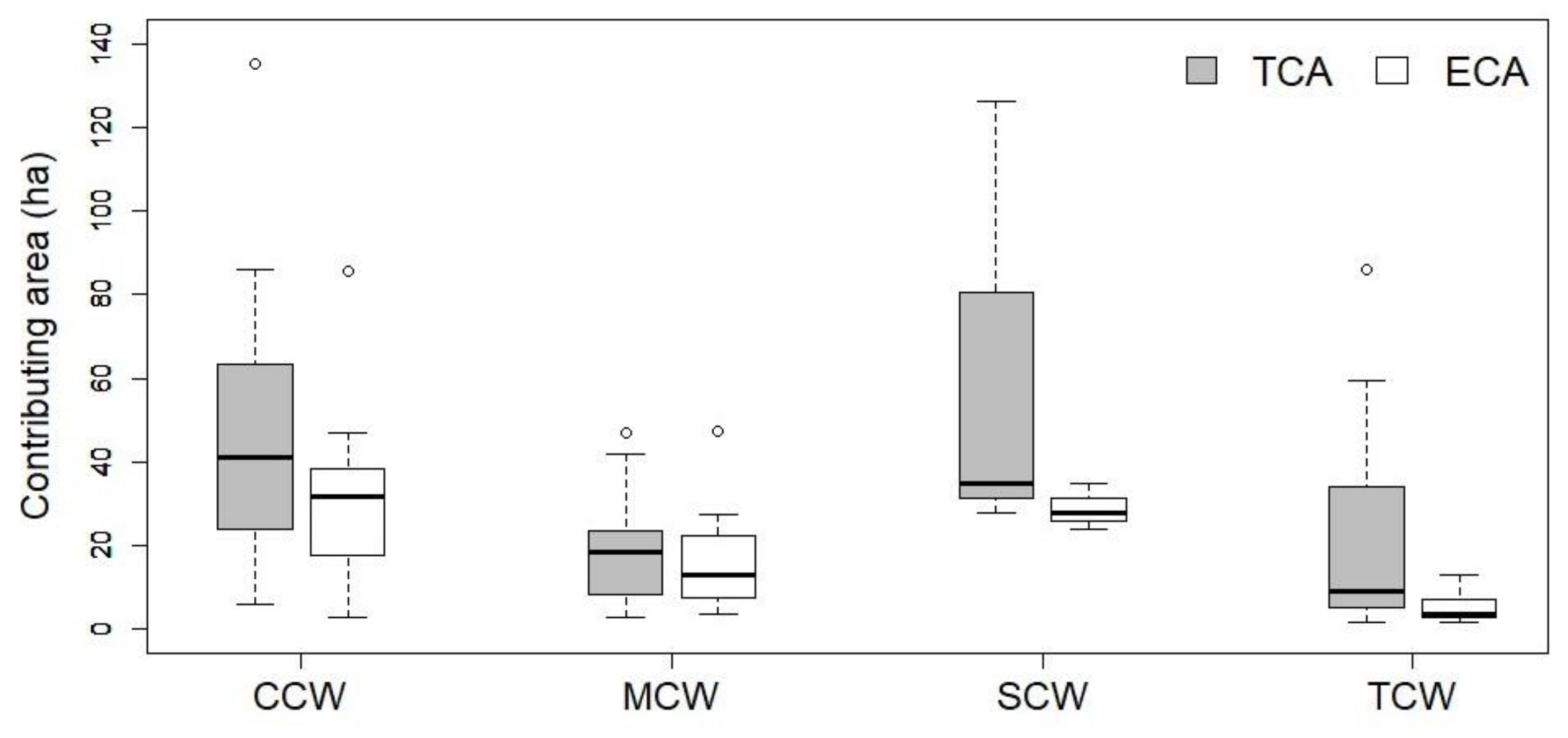
In TCW, eight of the 13 CP22 buffers that were assessed using topographic openness, were affected by concentrated flowpaths. These concentrated flowpaths were primarily in the form of micro-ditches that reduced the contributing areas that may be treated by the buffers by approximately 78%. In the MCW, 11 of the 25 CP22 buffers that were assessed using flow accumulation, were affected by concentrated flowpaths. These concentrated flowpaths were naturally occurring in most areas, and reduced the contributing areas that may be treated by the buffers by approximately 22%. In the SCW, one of the three (33%) CP22 buffers that were assessed using flow accumulation, was affected by concentrated flowpaths. These concentrated flowpaths were naturally occurring, and reduced the contributing areas that may be treated by the buffers by approximately 54%. In the CCW, seven of the 13 CP22 buffers that were assessed using flow accumulation, were affected by concentrated flowpaths. These concentrated flowpaths were naturally occurring in most areas, and reduced the contributing areas that may be treated by the buffers by approximately 38%.
4. Discussion
The results are discussed in two subsections. The first subsection compares the positive openness and flow accumulation across low and high relief regions; and the second subsection discusses the effects of hydrologic bypass features on riparian forest buffer contributing areas.
4.1. Performance of Topographic Metrics in Different Topographic Relief Areas
Topographic openness has been widely used in geomorphology studies [45,46,47,48], but is seldom used in hydrologic studies despite being identified as one of the most important topographic metrics that can be used to study flow patterns within a watershed [49]. The topographic openness maps generated in this study made it easy to visualize critical source areas, berms, and flow routing patterns using LiDAR-derived DEMs. These hydrologic features were more evident for all the CP22 buffer contributing areas in the Coastal Plains physiographic region. Being able to clearly identify critical source areas in the landscape is a major advantage of the topographic openness approach in low relief areas. This allows for a more targeted approach to reducing contaminants in surface runoff.
A critical source area is an indentation ranging from a small area trampled by cattle to a whole field that serves as a significant source of nutrient input. Concentrated flowpaths often provide direct connection between the critical source areas and the receiving waters. Heathwaite et al. [50], used topographic openness to develop a model that examined the contribution that critical source areas make to nutrient pollution in receiving waters. Other approaches have integrated topographic information with maps of soil hydrology to identify critical source areas. By identifying critical source areas, hydrological engineering or best management approaches may be adopted to mitigate this risk at a practical level [51,52].
Another feature that was noticeable with the topographic openness map was the presence of berms in riparian buffer zones, Figure 7. Berms are usually created during ditch digging, plowing or through the accumulation of sediment over time. They often restrict sheet flow and could reduce the velocity of flow through the riparian area, however, they ultimately back up surface runoff, resulting in an eventual breakthrough that concentrates overland flow [28].
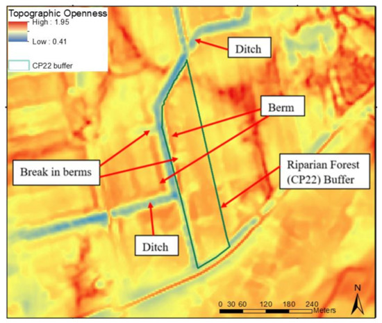
Figure 7.
A close-up of hydrologic features such as berms and ditches identified using topographic openness.
4.2. Effects of Hydrologic Bypass Features on CP22 Contributing Areas
The presence of hydrologic bypass features reduced the contributing areas that may be treated by the CP22 buffers (Figure 8) significantly (p < 0.05). Primarily, the effectiveness of riparian buffers in the TCW is being compromised by numerous in-field ditches, as shown in Figure 4A. These ditches short circuit the CP22 buffers put in place to mitigate agricultural pollution of surface waters. In contrast to the TCW, CP22 buffers in the SCW, CCW and MCW watersheds are affected by concentrated overland flows and not by manmade ditches. This is because farmers in the water-logged soils of the Coastal Plain use ditches to drain their fields quickly to maximize crop cultivation. In the higher relief areas, however, water logged soils is less of a problem for farmers, therefore fewer ditches are constructed in those areas.
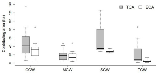
Figure 8.
Comparison of size distributions between topographic (TCA) and effective (ECA) contributing areas for each of CCW, MCW, SCW and TCW.
Naturally occurring concentrated flowpaths are more of a problem in the higher relief areas. The formation of concentrated flow paths within the buffer contributing areas in the higher relief watersheds are due to steep slopes and outcropping of different strata. In addition to steep slopes and outcropping, concentrated overland flows tend to occur more in rocky soils. Soils in the Piedmont, and Ridge and Valley physiographic region are mainly formed from sandstone, conglomerate, siltstone and limestone, compared to the loamy soils of the Coastal Plain. Therefore, despite having little to no manmade ditches that short-circuit CP22 buffers, the geomorphic conditions resulted in significant concentrated overland flow in CCW, MCW and SCW watersheds. As a result, more attention should be given to the topographic and geomorphic conditions of a watershed when designing and implementing CP22 buffers.
By limiting the proportion of surface runoff entering the buffer zones via sheet flow, concentrated flowpaths undermine the buffers’ ability to remove pollutants from overland flows. In a similar study conducted in a Southern Illinois watershed [52], it was found that 82.5 to 100 percent of surface runoff leaving the agricultural field occurs as concentrated flow. The number of concentrated flowpaths that fully transect a buffer, and those that originate from within each buffer varies. The implementation of conservation measures such as grassed waterways on concentrated flowpaths and filter strips at the edge of fields may help to reduce pollutant loadings by slowing overland flow, promoting infiltration and filtration, and establishing synergies with CP22 buffers. Use of controlled drainage structures such as flashboards or risers on ditches may help to restore the effectiveness of some of these CP22 buffers [53].
5. Conclusions
Examining flow routing patterns across a landscape is essential for correct buffer placement and for assessing the effectiveness of CP22 buffers in mitigating the impact of surface runoff and associated pollutant loadings. The results presented in this study demonstrate the ability of two topographic metrics to analyze and visualize overland flow routing patterns, which is important for good environmental conservation planning. The feasibility of using either the topographic openness or flow accumulation method relies on the availability of high resolution DEMs and on topographic relief. High resolution DEMs derived from LiDAR data provide highly detailed representations of the landscape when matched up against aerial photography. The two topographic visualization techniques examined in this study agreed with each other 100% of the time for the 52 CP22 buffers in the Chesapeake Bay Watershed. However, the flow accumulation technique displayed concentrated flowpaths best in medium to high and high relief areas such as those in the Piedmont and Appalachian Ridge and Valley physiographic provinces, when compared to topographic openness. The topographic openness on the other hand, worked best for displaying hydrologic features in low relief areas such as the Coastal Plain.
Results from this study also indicated that hydrologic bypass features occurred in approximately half of the study sites (27 of 52) across all four watersheds. Hydrologic bypass features, whether drainage ditches or concentrated overland flows, were found to reduce the potential contributing areas to CP22 buffers by as much as 78%. Thus, the effectiveness of CP22 buffers to intercept and reduce pollutant loadings from surface runoff were reduced significantly. Surface water quality may suffer in areas with poorly designed and poorly placed buffers. Therefore, conservation managers should consider the occurrence of hydrologic bypass features when designing and maintaining riparian buffers to protect stream water quality.
Acknowledgments
This project was funded by the United States Department of Agriculture (USDA)—Farm Service Agency (FSA), Agricultural Research Service (ARS), Natural Resources Conservation Service (NRCS), and the Conservation Effects Assessment Project (CEAP) Watershed Component. The senior author was supported as a post-doctoral scholar by Riparia at Penn State, a center in the Department of Geography. Additional support for this project was also provided by the Interstate Commission on the Potomac River Basin (ICPRB). Mention of trade names or commercial products in this publication is solely for the purpose of providing specific information and does not imply recommendation or endorsement by the U.S. Department of Agriculture (USDA). USDA is an equal opportunity provider and employer. The U.S. Department of Agriculture prohibits discrimination in all its programs and activities on the basis of race, color, national origin, age, disability, and where applicable, sex, marital status, familial status, parental status, religion, sexual orientation, genetic information, political beliefs, reprisal, or because all or part of an individual’s income is derived from any public assistance program. (Not all prohibited bases apply to all programs.) Persons with disabilities who require alternative means for communication of program information (Braille, large print, audiotape, etc.) should contact USDA’s TARGET Center at (202) 720-2600 (voice and TDD). To file a complaint of discrimination, write to USDA, Director, Office of Civil Rights, 1400 Independence Avenue, S.W., Washington, D.C. 20250-9410, or call (800) 795-3272 (voice) or (202) 720-6382 (TDD).
Author Contributions
C.W.W. developed methodology and performed most analysis and writing; S.L. performed analysis and helped with writing; G.M. lead the data collection and supervised the project; R.P.B. and P.J.A.K. were instrumental in conceiving the study and managing the project; T.L.V. and A.M.S. were instrumental in writing, data analysis and QAQC.
Conflicts of Interest
The authors declare no conflict of interest. The funding sponsors had no role in the design of the study, in the collection, analyses, or interpretation of data, in the writing of the manuscript, and in the decision to publish the results.
References
- Hirsch, R.M.; Moyer, D.L.; Archfield, S.A. Weighted regressions on time, discharge, and season (wrtds), with an application to Chesapeake Bay river inputs. J. Am. Water Resour. Assoc. 2010, 46, 857–880. [Google Scholar] [CrossRef] [PubMed]
- Russell, K.M.; Galloway, J.N.; Macko, S.A.; Moody, J.L.; Scudlark, J.R. Sources of nitrogen in wet deposition to the Chesapeake Bay region. Atmos. Environ. 1998, 32, 2453–2465. [Google Scholar] [CrossRef]
- Owens, M.; Cornwell, J.C. Sedimentary evidence for decreased heavy-metal inputs to the chesapeake bay. Ambio 1995, 24, 24–27. [Google Scholar]
- Shuyler, L.R.; Linker, L.C.; Walters, C.P. The Chesapeake Bay story—The science behind the program. Water Sci. Technol. 1995, 31, 133–139. [Google Scholar]
- Bauereis, E.I. Chesapeake experience—NPS Chesapeake challenge for sustainable development. Water Sci. Technol. 1992, 26, 2723–2725. [Google Scholar]
- Leight, A.K.; Slacum, W.H.; Wirth, E.F.; Fulton, M.H. An assessment of benthic condition in several small watersheds of the Chesapeake Bay, USA. Environ. Monit. Assess. 2011, 176, 483–500. [Google Scholar] [CrossRef] [PubMed]
- Inamdar, S.P.; Mostaghimi, S.; McClellan, P.W.; Brannan, K.M. BMP impacts on sediment and nutrient yields from an agricultural watershed in the Coastal Plain region. Trans. ASAE 2001, 44, 1191–1200. [Google Scholar] [CrossRef]
- Welsch, D.J. Riparian Forest Buffers: Function and Design for Protection and Enhancement of Water Resources; U.S. Department of Agriculture, Forest Service, Northeastern Area, State & Private Forestry, Forest Resources Management: Newtown Square, PA, USA, 1991; Volume 7.
- Sheridan, J.M.; Lowrance, R.; Bosch, D.D. Management effects on runoff and sediment transport in riparian forest buffers. Trans. ASAE 1999, 42, 55–64. [Google Scholar] [CrossRef]
- Lee, K.H.; Isenhart, T.M.; Schultz, R.C. Sediment and nutrient removal in an established multi-species riparian buffer. J. Soil Water Conserv. 2003, 58, 1–8. [Google Scholar]
- Jordan, T.; Correll, D.; Weller, D. Nutrient interception by a riparian forest receiving inputs from adjacent cropland. J. Environ. Qual. 1993, 22, 467–473. [Google Scholar] [CrossRef]
- Lowrance, R.; Altier, L.; Newbold, J.; Schnabel, R.; Groffman, P.; Denver, J.; Correll, D.; Gilliam, J.; Robinson, J.; Brinsfield, R.; et al. Water quality functions of riparian forest buffers in Chesapeake Bay watersheds. Environ. Manag. 1997, 21, 687–712. [Google Scholar] [CrossRef]
- Angier, J.; McCarty, G.; Prestegaard, K. Hydrology of a first-order riparian zone and stream, Mid-Atlantic Coastal Plain, Maryland. J. Hydrol. 2005, 309, 149–166. [Google Scholar] [CrossRef]
- Angier, J.; McCarty, G. Variations in base-flow nitrate flux in a first-order stream and riparian zone. J. Am. Water Resour. Assoc. 2008, 44, 367–380. [Google Scholar] [CrossRef]
- Shoemaker, R. The Conservation Reserve Program and Its Effect on Land Values; U.S. Department of Agriculture, Economic Research Service: Washington, DC, USA, 1989.
- Dosskey, M.G.; Helmers, M.J.; Eisenhauer, D.E.; Franti, T.G.; Hoagland, K.D. Assessment of concentrated flow through riparian buffers. J. Soil Water Conserv. 2002, 57, 336–343. [Google Scholar]
- Knight, K.W.; Schultz, R.C.; Mabry, C.M.; Isenhart, T.M. Ability of remnant riparian forests, with and without grass filters, to buffer concentrated surface runoff1. J. Am. Water Resour. Assoc. 2010, 46, 311–322. [Google Scholar] [CrossRef]
- Lyons, J.; Trimble, S.W.; Paine, L.K. Grass versus trees: Managing riparian areas to benefit streams of Central North America. J. Am. Water Resour. Assoc. 2000, 36, 919–930. [Google Scholar] [CrossRef]
- Myers, J.L.; Wagger, M.G.; Leidy, R.B. Chemical movement in relation to tillage system and simulated rainfall intensity. J. Environ. Qual. 1995, 24, 1183–1192. [Google Scholar] [CrossRef]
- Schultz, R.C.; Isenhart, T.M.; Simpkins, W.W.; Colletti, J.P. Riparian forest buffers in agroecosystems—Lessons learned from the Bear Creek watershed, Central Iowa, USA. Agrofor. Syst. 2004, 63, 35–50. [Google Scholar]
- Dillaha, T.A.; Sherrard, J.H.; Lee, D.; Mostaghimi, S.; Shanholtz, V.O. Evaluation of vegetative filter strips as a best management practice for feed lots. J. Water Pollut. Control Fed. 1988, 60, 1231–1238. [Google Scholar]
- Dillaha, T.A.; Reneau, R.B.; Mostaghimi, S.; Lee, D. Vegetative filter strips for agricultural nonpoint source pollution-control. Trans. ASAE 1989, 32, 513–519. [Google Scholar] [CrossRef]
- Daniels, R.B.; Gilliam, J.W. Sediment and chemical load reduction by grass and riparian filters. Soil Sci. Soc. Am. J. 1996, 60, 246–251. [Google Scholar] [CrossRef]
- Pankau, R.C.; Schoonover, J.E.; Williard, K.W.J.; Edwards, P.J. Concentrated flow paths in riparian buffer zones of Southern Illinois. Agrofor. Syst. 2012, 84, 191–205. [Google Scholar] [CrossRef]
- Mayer, P.; Reynolds, S.; McCutchen, M.; Canfield, T. Meta-analysis of nitrogen removal in riparian buffers. J. Environ. Qual. 2007, 36, 1172–1180. [Google Scholar] [CrossRef] [PubMed]
- Lee, K.; Isenhart, T.; Schultz, R.; Mickelson, S. Multispecies riparian buffers trap sediment and nutrients during rainfall simulations. J. Environ. Qual. 2000, 29, 1200–1205. [Google Scholar] [CrossRef]
- Liu, X.; Mang, X.; Zhang, M. Major factors influencing the efficacy of vegetated buffers on sediment trapping: A review and analysis. J. Environ. Qual. 2008, 37, 1667–1674. [Google Scholar] [CrossRef] [PubMed]
- Fox, G.; Sabbagh, G. Comment on “Major factors influencing the efficacy of vegetated buffers on sediment trapping: A review and analysis,” By xingmei liu, xuyang zhang, and minghua zhang in the journal of environmental quality 2008 37:1667-1674. J. Environ. Qual. 2009, 38, 1–2. [Google Scholar] [CrossRef] [PubMed]
- Piechnik, D.; Goslee, S.; Veith, T.; Bishop, J.; Brooks, R. Topographic placement of management practices in riparian zones to reduce water quality impacts from pastures. Landsc. Ecol. 2012, 27, 1307–1319. [Google Scholar] [CrossRef]
- Mausbach, M.; Dedrick, A. The length we go—Measuring environmental benefits of conservation practices. J. Soil Water Conserv. 2004, 59, 96A–103A. [Google Scholar]
- Wallace, C.; Flanagan, D.; Engel, B. Quantifying the effects of conservation practice implementation on predicted runoff and chemical losses under climate change. Agric. Water Manag. 2017, 186, 51–65. [Google Scholar] [CrossRef]
- Walbridge, M.R.; Shafer, S.R. A long-term agroecosystem research (ltar) network for agriculture. In Proceedings of the Fourth Interagency Conference on Research in the Watersheds, Fairbanks, AK, USA, 26–30 September 2011. [Google Scholar]
- USDA-NRCS (United States Department of Agriculture, N.R.C.S.). Official Soil Series Descriptions. Available online: https://soilseries.sc.egov.usda.gov/osdlist.aspx (accessed on 14 November 2017).
- Foyle, A.M.; Oertel, G.F. Seismic stratigraphy and coastal drainage patterns in the Quaternary section of the Southern Delmarva Peninsula, Virginia, USA. Sediment. Geol. 1992, 80, 261–277. [Google Scholar] [CrossRef]
- McCarty, G.; McConnell, L.; Hapernan, C.; Sadeghi, A.; Graff, C.; Hively, W.; Lang, M.; Fisher, T.; Jordan, T.; Rice, C.; et al. Water quality and conservation practice effects in the Choptank River watershed. J. Soil Water Conserv. 2008, 63, 461–474. [Google Scholar] [CrossRef]
- Bryant, R.; Veith, T.; Feyereisen, G.; Buda, A.; Church, C.; Folmar, G.; Schmidt, J.; Dell, C.; Kleinman, P. US Department of Agriculture Agricultural Research Service Mahantango Creek watershed, Pennsylvania, United States: Physiography and history. Water Resour. Res. 2011, 47, 8. [Google Scholar] [CrossRef]
- White, K.E. Regional Curve Development and Selection of a Reference Reach in the Non-Urban, Lowland Sections of the Piedmont Physiographic Province, Pennsylvania and Maryland; Pennsylvania Water Science Center: New Cumberland, PA, USA, 2001; 20p.
- Lang, M.; McCarty, G.; Oesterling, R.; Yeo, I. Topographic metrics for improved mapping of forested wetlands. Wetlands 2013, 33, 141–155. [Google Scholar] [CrossRef]
- Lang, M.; McCarty, G. LiDAR intensity for improved detection of inundation below the forest canopy. Wetlands 2009, 29, 1166–1178. [Google Scholar] [CrossRef]
- Carline, R.; Walsh, M. Responses to riparian restoration in the Spring Creek watershed, Central Pennsylvania. Restor. Ecol. 2007, 15, 731–742. [Google Scholar] [CrossRef]
- Conrad, O.; Bechtel, B.; Bock, M.; Dietrich, H.; Fischer, E.; Gerlitz, L.; Wehberg, J.; Wichmann, V.; Bohner, J. System for Automated Geoscientific Analyses (SAGA) v. 2.1.4. Geosci. Model. Dev. 2015, 8, 1991–2007. [Google Scholar] [CrossRef]
- Li, X.; McCarty, G.; Karlen, D.; Cambardella, C. Topographic metric predictions of soil redistribution and organic carbon in Iowa cropland fields. Catena 2018, 160, 222–232. [Google Scholar] [CrossRef]
- Yokoyama, R.; Shirasawa, M.; Pike, R. Visualizing topography by openness: A new application of image processing to digital elevation models. Photogramm. Eng. Remote Sens. 2002, 68, 257–265. [Google Scholar]
- Tarboton, D. A new method for the determination of flow directions and upslope areas in grid digital elevation models. Water Resour. Res. 1997, 33, 309–319. [Google Scholar] [CrossRef]
- Chu, H.; Huang, M.; Tain, Y.; Yang, M.; Hofle, B. Historic low wall detection via topographic parameter images derived from fine-resolution dem. ISPRS Int. J. Geo-Inf. 2017, 6, 346. [Google Scholar] [CrossRef]
- Prima, O.; Echigo, A.; Yokoyama, R.; Yoshida, T. Supervised landform classification of Northeast Honshu from dem-derived thematic maps. Geomorphology 2006, 78, 373–386. [Google Scholar] [CrossRef]
- Prima, O.; Yoshida, T. Characterization of volcanic geomorphology and geology by slope and topographic openness. Geomorphology 2010, 118, 22–32. [Google Scholar] [CrossRef]
- Inomata, T.; Pinzon, F.; Ranchos, J.; Haraguchi, T.; Nasu, H.; Fernandez-Diaz, J.; Aoyama, K.; Yonenobu, H. Archaeological application of airborne LiDAR with object-based vegetation classification and visualization techniques at the Lowland Maya site of Ceibal, Guatemala. Remote Sens. 2017, 9, 563. [Google Scholar] [CrossRef]
- Li, X.; McCarty, G.; Lang, M.; Ducey, T.; Hunt, P.; Miller, J. Topographic and physicochemical controls on soil denitrification in prior converted croplands located on the Delmarva Peninsula, USA. Geoderma 2018, 309, 41–49. [Google Scholar] [CrossRef]
- Heathwaite, A.; Quinn, P.; Hewett, C. Modelling and managing critical source areas of diffuse pollution from agricultural land using flow connectivity simulation. J. Hydrol. 2005, 304, 446–461. [Google Scholar] [CrossRef]
- Ghebremichael, L.; Veith, T.; Hamlett, J. Integrated watershed- and farm-scale modeling framework for targeting critical source areas while maintaining farm economic viability. J. Environ. Manag. 2013, 114, 381–394. [Google Scholar] [CrossRef] [PubMed]
- Ghebremichael, L.; Watzin, M. Identifying and controlling critical sources of farm phosphorus imbalances for Vermont dairy farms. Agric. Syst. 2011, 104, 551–561. [Google Scholar] [CrossRef]
- Gilliam, J.; Skaggs, R.; Weed, S. Drainage control to diminish nitrate loss from agricultural fields. J. Environ. Qual. 1979, 8, 137–142. [Google Scholar] [CrossRef]


© 2018 by the authors. Licensee MDPI, Basel, Switzerland. This article is an open access article distributed under the terms and conditions of the Creative Commons Attribution (CC BY) license (http://creativecommons.org/licenses/by/4.0/).