A WFS-SVM Model for Soil Salinity Mapping in Keriya Oasis, Northwestern China Using Polarimetric Decomposition and Fully PolSAR Data

 ,
,  ,
,  ,
,
Abstract
:
1. Introduction
2. Study Site and Data
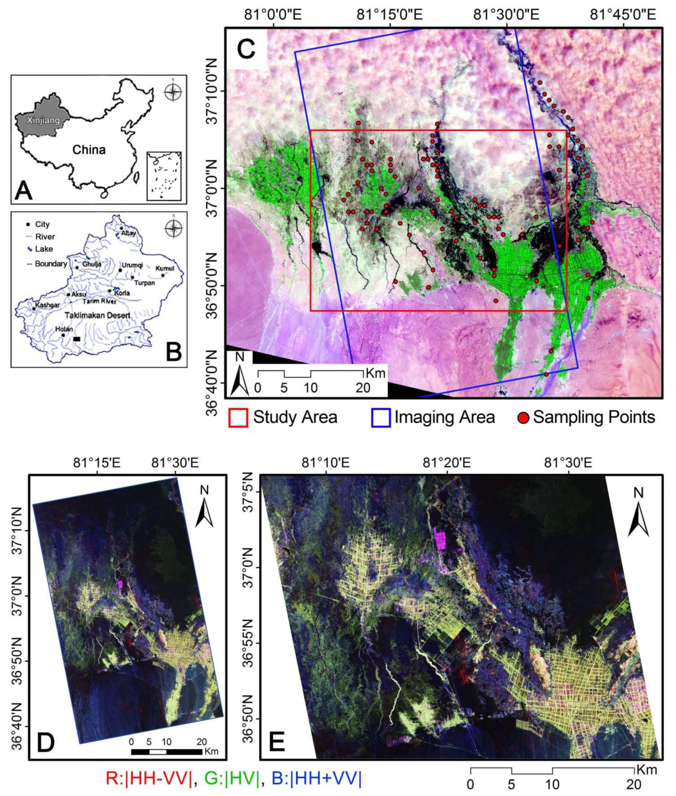
2.1. Study Site
2.2. Data
2.2.1. Remote Sensing Data
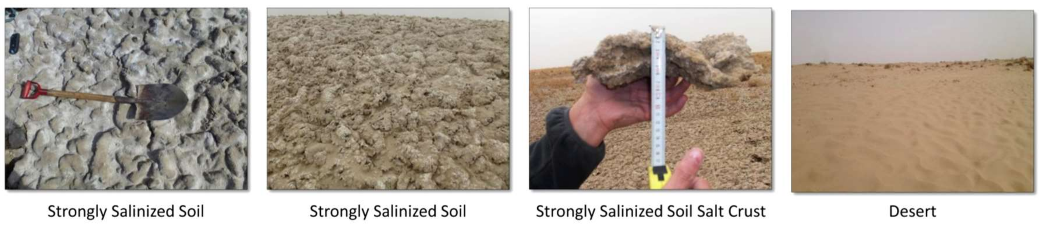
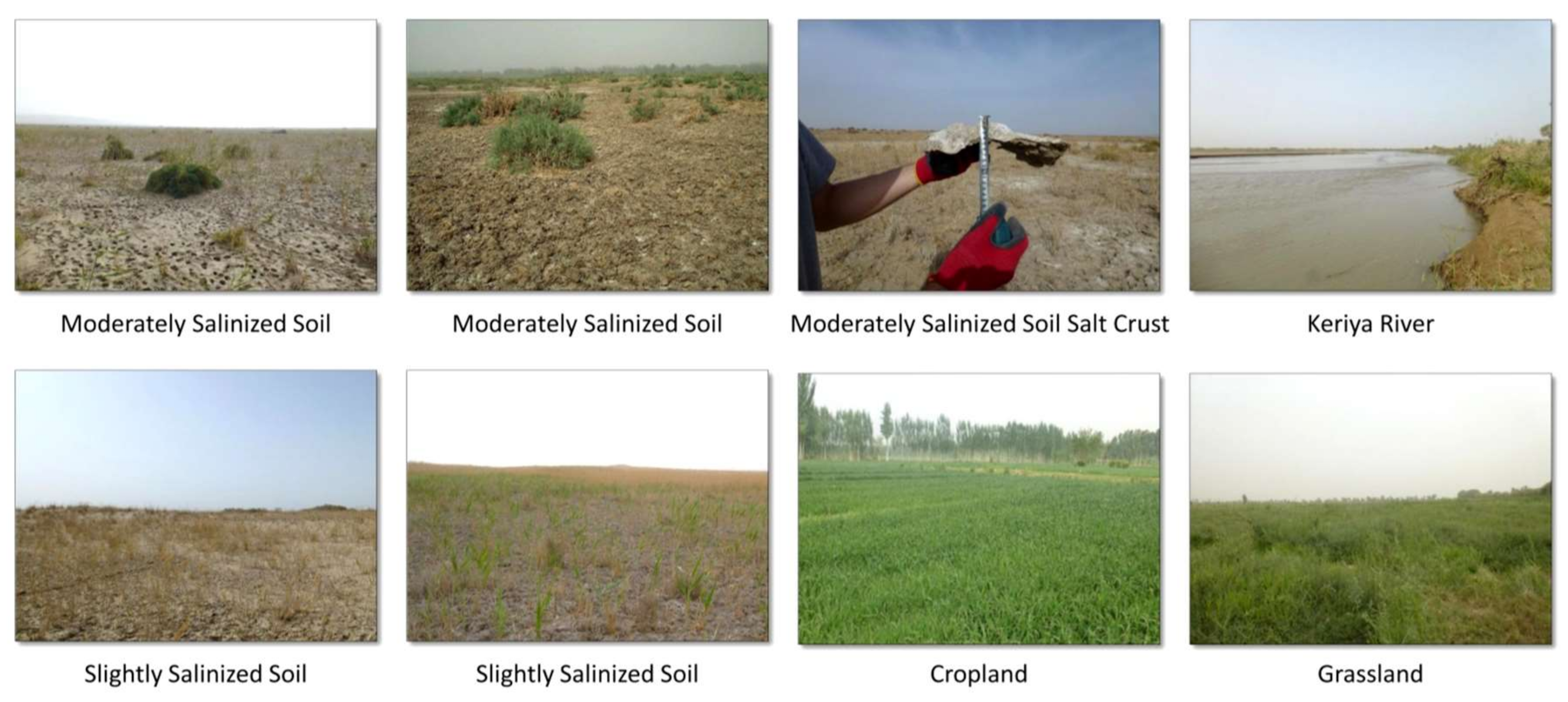
2.2.2. Field Data
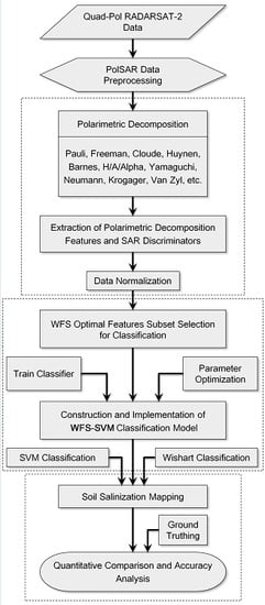
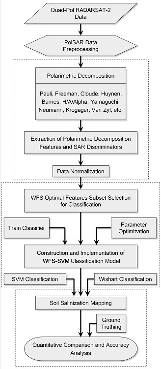
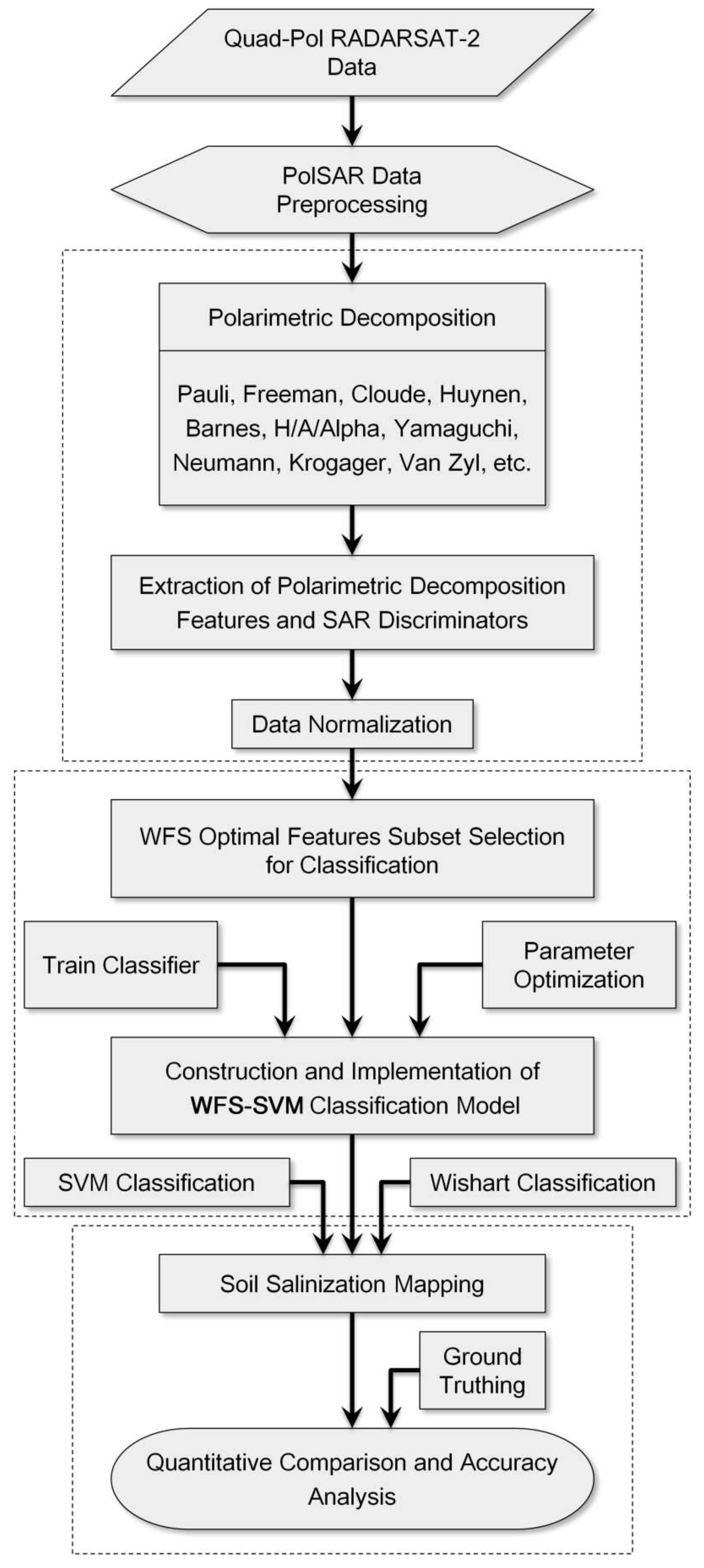
3. Methodology
3.1. Polarimetric Decomposition
3.2. Wrapper Feature Selector (WFS)
3.3. Support Vector Machine (SVM) Classification
4. Results
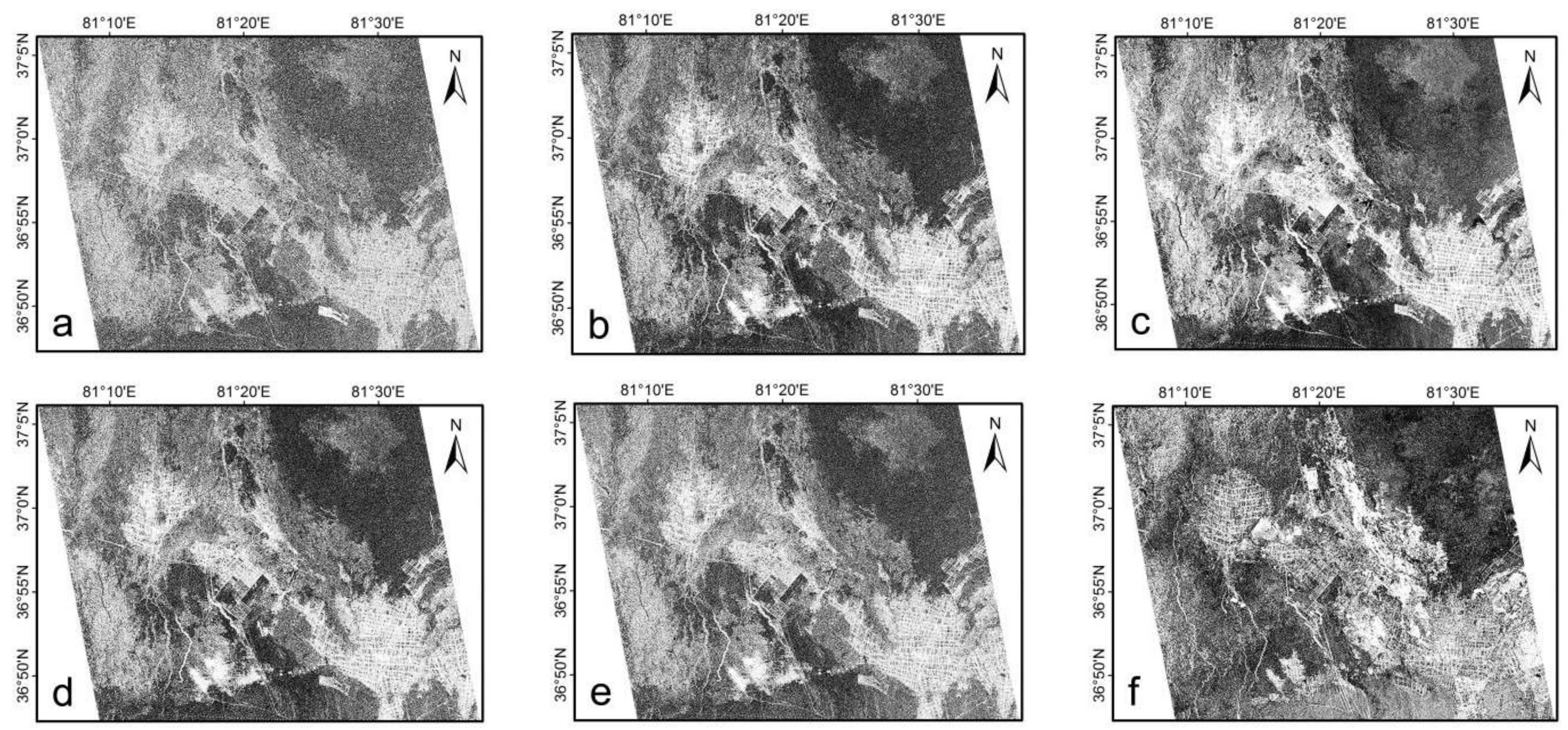
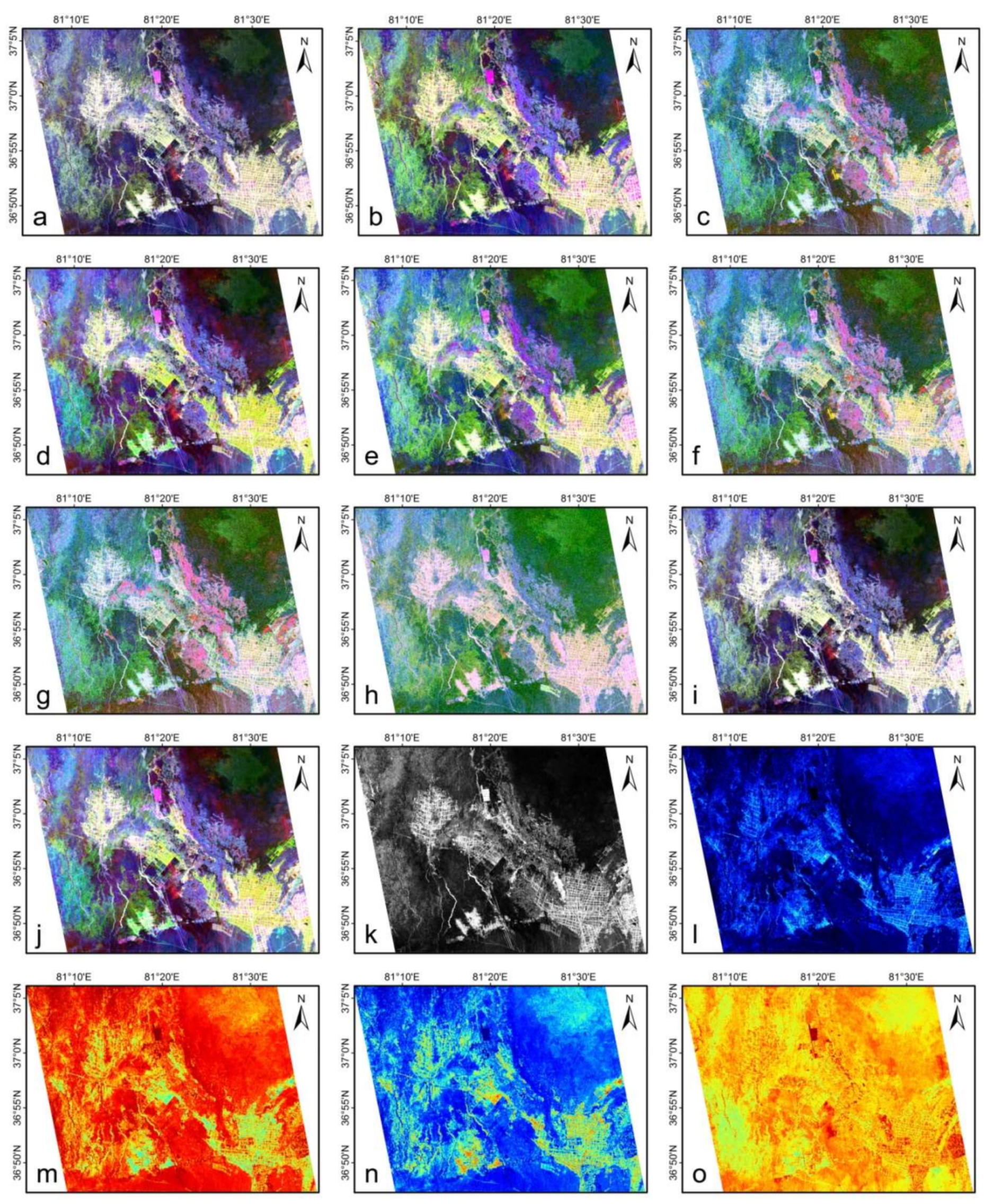
4.1. Polarimetric Decomposition of Fully PolSAR Data
4.2. Construction of WFS-SVM Classification Model
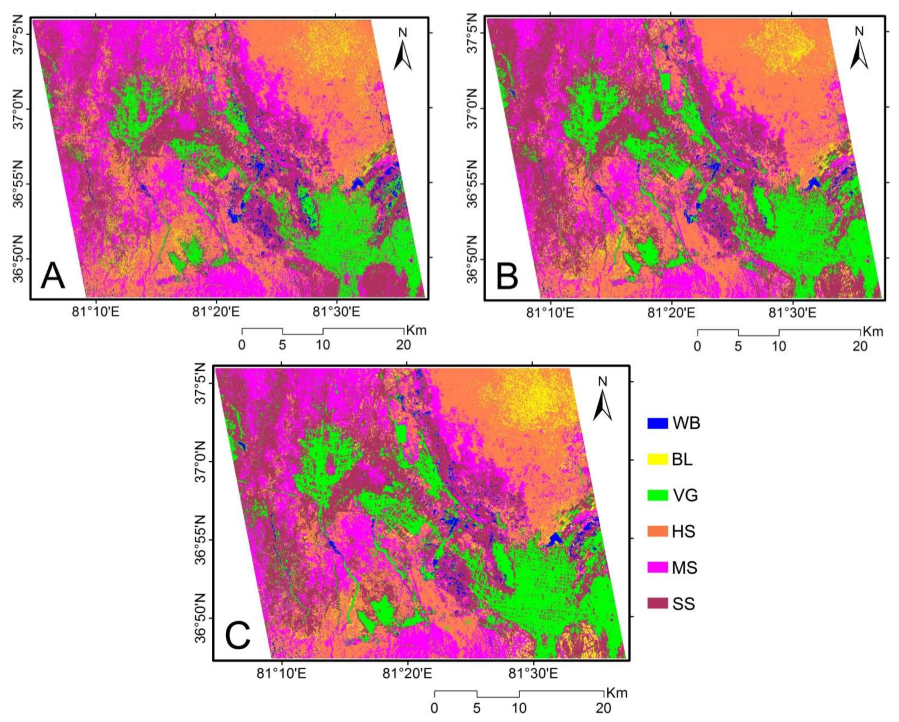
4.3. Soil Salinity Mapping
4.4. Accuracy Assessment
5. Discussion
6. Conclusions
Acknowledgments
Author Contributions
Conflicts of Interest
References
- Metternicht, G.I.; Zinck, J.A. Remote sensing of soil salinity: Potentials and constraints. Remote Sens. Environ. 2003, 85, 1–20. [Google Scholar] [CrossRef]
- Farifteh, J.; Farshad, A.; George, R.J. Assessing salt-affected soils using remote sensing, solute modelling, and geophysics. Geoderma 2006, 130, 191–206. [Google Scholar] [CrossRef]
- Sidike, A.; Zhao, S.; Wen, Y. Estimating soil salinity in Pingluo County of China using QuickBird data and soil reflectance spectra. Int. J. Appl. Earth Obs. Geoinf. 2014, 26, 156–175. [Google Scholar] [CrossRef]
- Odeh, I.O.A.; Onus, A. Spatial Analysis of Soil Salinity and Soil Structural Stability in a Semiarid Region of New South Wales, Australia. Environ. Manag. 2008, 42, 265. [Google Scholar] [CrossRef] [PubMed]
- Abdelfattah, A.M.; Shahid, A.S.; Othman, R.Y. Soil Salinity Mapping Model Developed Using RS and GIS—A Case Study from Abu Dhabi, United Arab Emirates. Eur. J. Sci. Res. 2009, 26, 342–351. [Google Scholar]
- Allbed, A.; Kumar, L. Soil Salinity Mapping and Monitoring in Arid and Semi-Arid Regions Using Remote Sensing Technology: A Review. Adv. Remote Sens. 2013, 2, 373–385. [Google Scholar] [CrossRef]
- Nurmemet, I.; Ghulam, A.; Tiyip, T.; Elkadiri, R.; Ding, J.L.; Maimaitiyiming, M.; Abliz, A.; Sawut, M.; Zhang, F.; Abliz, A.; et al. Monitoring soil salinization in Keriya River Basin, Northwestern China using passive reflective and active microwave remote sensing data. Remote Sens. 2015, 7, 8803–8829. [Google Scholar] [CrossRef]
- Douaoui, A.E.K.; Nicolas, H.; Walter, C. Detecting salinity hazards within a semiarid context by means of combining soil and remote-sensing data. Geoderma 2006, 134, 217–230. [Google Scholar] [CrossRef]
- Fernández-Buces, N.; Siebe, C.; Cram, S.; Palacio, J.L. Mapping soil salinity using a combined spectral response index for bare soil and vegetation: A case study in the former lake Texcoco, Mexico. J. Arid Environ. 2006, 65, 644–667. [Google Scholar] [CrossRef]
- Allbed, A.; Kumar, L.; Sinha, P. Mapping and Modelling Spatial Variation in Soil Salinity in the Al Hassa Oasis Based on Remote Sensing Indicators and Regression Techniques. Remote Sens. 2014, 6, 1137–1157. [Google Scholar] [CrossRef]
- Metternicht, G.; Zinck, A. Remote Sensing of Soil Salinization: Impact on Land Management; CRC Press: Boca Raton, FL, USA, 2008; ISBN 1420065033. [Google Scholar]
- Mulder, V.L.; De Bruin, S.; Schaepman, M.E.; Mayr, T.R. The use of remote sensing in soil and terrain mapping—A review. Geoderma 2011, 162, 1–19. [Google Scholar] [CrossRef]
- Corwin, D.L.; Plant, R.E. Applications of apparent soil electrical conductivity in precision agriculture. Comput. Electron. Agric. 2005, 46, 1–10. [Google Scholar] [CrossRef]
- Rhoades, J.D.; Chanduvi, F. Soil Salinity Assessment: Methods and Interpretation of Electrical Conductivity Measurements; Food & Agriculture Organazition: Rome, Italy, 1999; Volume 57, ISBN 9251042810. [Google Scholar]
- Bell, D.; Menges, C.; Ahmad, W.; Van Zyl, J.J. The application of dielectric retrieval algorithms for mapping soil salinity in a tropical coastal environment using airborne polarimetric SAR. Remote Sens. Environ. 2001, 75, 375–384. [Google Scholar] [CrossRef]
- Lasne, Y.; Paillou, P.; Freeman, A.; Farr, T.; McDonald, K.C.; Ruffie, G.; Malezieux, J.-M.; Chapman, B.; Demontoux, F. Effect of salinity on the dielectric properties of geological materials: Implication for soil moisture detection by means of radar remote sensing. IEEE Trans. Geosci. Remote Sens. 2008, 46, 1674–1688. [Google Scholar] [CrossRef]
- Grissa, M.; Abdelfattah, R.; Mercier, G.; Zribi, M.; Chahbi, A.; Lili-Chabaane, Z. Empirical model for soil salinity mapping from SAR data. In Proceedings of the IEEE International Geoscience and Remote Sensing Symposium (IGARSS), Vancouver, BC, Canada, 24–29 July 2011; pp. 1099–1102. [Google Scholar]
- Qi, Z.; Yeh, A.G.-O.; Li, X.; Lin, Z. A novel algorithm for land use and land cover classification using RADARSAT-2 polarimetric SAR data. Remote Sens. Environ. 2012, 118, 21–39. [Google Scholar] [CrossRef]
- Bindlish, R.; Barros, A.P. Parameterization of vegetation backscatter in radar-based, soil moisture estimation. Remote Sens. Environ. 2001, 76, 130–137. [Google Scholar] [CrossRef]
- Maghsoudi, Y.; Collins, M.J.; Leckie, D.G. Radarsat-2 polarimetric SAR data for boreal forest classification using SVM and a wrapper feature selector. IEEE J. Sel. Top. Appl. Earth Obs. Remote Sens. 2013, 6, 1531–1538. [Google Scholar] [CrossRef]
- Del Frate, F.; Ferrazzoli, P.; Schiavon, G. Retrieving soil moisture and agricultural variables by microwave radiometry using neural networks. Remote Sens. Environ. 2003, 84, 174–183. [Google Scholar] [CrossRef]
- Serbin, G.; Or, D. Ground-penetrating radar measurement of soil water content dynamics using a suspended horn antenna. IEEE Trans. Geosci. Remote Sens. 2004, 42, 1695–1705. [Google Scholar] [CrossRef]
- Zhu, Z.; Woodcock, C.E.; Rogan, J.; Kellndorfer, J. Assessment of spectral, polarimetric, temporal, and spatial dimensions for urban and peri-urban land cover classification using Landsat and SAR data. Remote Sens. Environ. 2012, 117, 72–82. [Google Scholar] [CrossRef]
- Amarsaikhan, D.; Douglas, T. Data fusion and multisource image classification. Int. J. Remote Sens. 2004, 25, 3529–3539. [Google Scholar] [CrossRef]
- Shao, Y.; Hu, Q.; Guo, H.; Lu, Y.; Dong, Q.; Han, C. Effect of dielectric properties of moist salinized soils on backscattering coefficients extracted from RADARSAT image. IEEE Trans. Geosci. Remote Sens. 2003, 41, 1879–1888. [Google Scholar] [CrossRef]
- Shimoni, M.; Borghys, D.; Heremans, R.; Perneel, C.; Acheroy, M. Fusion of PolSAR and PolInSAR data for land cover classification. Int. J. Appl. Earth Obs. Geoinf. 2009, 11, 169–180. [Google Scholar] [CrossRef]
- Huang, L.; Li, Z.; Tian, B.-S.; Chen, Q.; Liu, J.-L.; Zhang, R. Classification and snow line detection for glacial areas using the polarimetric SAR image. Remote Sens. Environ. 2011, 115, 1721–1732. [Google Scholar] [CrossRef]
- Chen, S.W.; Li, Y.Z.; Wang, X.S.; Xiao, S.P. Modeling and Interpretation of Scattering Mechanisms in Polarimetric Synthetic Aperture Radar: Advances and perspectives. Signal Process. Mag. IEEE 2014, 31, 79–89. [Google Scholar] [CrossRef]
- Tiyip, T.; Ding, J. Oasis Remote Sensing; Xinjiang People’s Publishing House: Xinjiang, China, 2009. [Google Scholar]
- Abliz, A.; Tiyip, T.; Ghulam, A.; Halik, Ü.; Ding, J.-L.; Sawut, M.; Zhang, F.; Nurmemet, I.; Abliz, A. Effects of shallow groundwater table and salinity on soil salt dynamics in the Keriya Oasis, Northwestern China. Environ. Earth Sci. 2016, 75, 260. [Google Scholar] [CrossRef]
- Gong, L.; Ran, Q.; He, G.; Tiyip, T. A soil quality assessment under different land use types in Keriya river basin, Southern Xinjiang, China. Soil Tillage Res. 2015, 146, 223–229. [Google Scholar] [CrossRef]
- Mu, Q.; Zi-an, Z.; Hong, M. Survey on the Arable Land Resource of Xinjiang Based on Remote Sensing; Science and Technology Publishing House of Xinjiang: Xinjiang, China, 2005. [Google Scholar]
- Tiyip, T.; Fei, Z.; Jianli, D. Study on the spatial information on salinized soil of typical oases in arid areas. Arid L. Geogr. 2007, 544–551. [Google Scholar]
- Yang, X. The oases along the Keriya River in the Taklamakan Desert, China, and their evolution since the end of the last glaciation. Environ. Geol. 2001, 41, 314–320. [Google Scholar] [CrossRef]
- Yang, X. The relationship between oases evolution and natural as well as human factors-evidences from the lower reaches of the Keriya River, southern Xinjiang, China. Earth Sci. Front. 2001, 8, 83–90. [Google Scholar]
- Ling, H.; Xu, H.; Zhang, Q. Nonlinear analysis of runoff change and climate factors in the headstream of Keriya River, Xinjiang. Geogr. Res. 2012, 31, 792–802. [Google Scholar]
- Yuquan, L. The Climatic Characteristics and Its Changing Tendency in the Taklimakan Desert. J. Desert Res. 1990, 2, 9–19. [Google Scholar]
- Sawut, M.; Ghulam, A.; Tiyip, T.; Zhang, Y.; Ding, J.; Zhang, F.; Maimaitiyiming, M. Estimating soil sand content using thermal infrared spectra in arid lands. Int. J. Appl. Earth Obs. Geoinf. 2014, 33, 203–210. [Google Scholar] [CrossRef]
- Hu, X. Study of Relationship between the Soil-Salinization and the Change of Groundwater Environment in Yutian Oasis; Xinjiang University: Xinjiang, China, 2008. [Google Scholar]
- Suzuki, S.; Kankaku, Y.; Osawa, Y. Development Status of PALSAR-2 onboard ALOS-2. In SPIE Remote Sensing; International Society for Optics and Photonics: Bellingham, WA, USA, 2011; p. 81760Q. [Google Scholar]
- Arikawa, Y.; Saruwatari, H.; Hatooka, Y.; Suzuki, S. ALOS-2 launch and early orbit operation result. Int. Geosci. Remote Sens. Symp. 2014, 2, 3406–3409. [Google Scholar] [CrossRef]
- Kankaku, Y.; Sagisaka, M.; Suzuki, S. PALSAR-2 launch and early orbit status. Int. Geosci. Remote Sens. Symp. 2014, 2, 3410–3412. [Google Scholar] [CrossRef]
- Lopes, A.; Touzi, R.; Nezry, E. Adaptive speckle filters and scene heterogeneity. IEEE Trans. Geosci. Remote Sens. 1990, 28, 992–1000. [Google Scholar] [CrossRef]
- Holecz, F.; Meier, E.; Piesbergen, J.; Nisch, D.; Moreira, J. Rigorous Derivation of Backscattering Coefficient. IEEE Geosc. Remote Sens. Soc. Newsl. 1994, 92, 6–14. [Google Scholar]
- Sarmap SA. Synthetic Aperture Radar and SARscape: SAR Guidebook; Sarmap SA: Purasca, Switzerland, 2009. [Google Scholar]
- Ulaby, F.T.; Dobson, M.C. Handbook of Radar Scattering Statistics for Terrain; Artech House: Norwood, MA, USA, 1989; Volume 1, ISBN 0890063362. [Google Scholar]
- Ilyas, N.; Tashpolat, T.; Ding, J.; Mamat, S.; Zhang, F.; Sun, Q. Monitoring soil salinization in arid area using PolSAR data and polarimetric decomposition method. Trans. Chin. Soc. Agric. Eng. 2015, 49, 698–707. [Google Scholar]
- Trudel, M.; Magagi, R.; Granberg, H.B. Application of target decomposition theorems over snow-covered forested areas. IEEE Trans. Geosci. Remote Sens. 2009, 47, 508–512. [Google Scholar] [CrossRef]
- Touzi, R. Target scattering decomposition in terms of roll-invariant target parameters. IEEE Trans. Geosci. Remote Sens. 2007, 45, 73–84. [Google Scholar] [CrossRef]
- Huynen, J.R. Phenomenological Theory of Radar Targets; Delft University of Technology: Delft, The Netherlands, 1970. [Google Scholar]
- Mishra, P.; Singh, D.; Yamaguchi, Y.; Singh, D. Land Cover Classification of Palsar Images By Knowledge Based Decision Tree Classi-Fier and Supervised Classifiers Based on Sar Observables. Prog. Electromagn. Res. B 2011, 30, 47–70. [Google Scholar] [CrossRef]
- An, W.; Cui, Y.; Yang, J. Three-component model-based decomposition for polarimetric sar data. IEEE Trans. Geosci. Remote Sens. 2010, 48, 2732–2739. [Google Scholar] [CrossRef]
- Cloude, S.R.; Pottier, E. A review of target decomposition theorems in radar polarimetry. IEEE Trans. Geosci. Remote Sens. 1996, 34, 498–518. [Google Scholar] [CrossRef]
- Lee, J.-S.; Pottier, E. Polarimetric Radar Imaging: From Basics to Applications; CRC press: Raton, FL, USA, 2009; ISBN 1420054988. [Google Scholar]
- Barnes, R.M. Roll invariant decompositions for the polarization covariance matrix. In Proceedings of the Polarimetry Technology Workshop, Redstone Arsenal, AL, USA, 16–18 August 1988. [Google Scholar]
- Cloude, S.R. Target decomposition theorems in radar scattering. Electron. Lett. 1985, 21, 22–24. [Google Scholar] [CrossRef]
- Holm, W.A.; Barnes, R.M. On Radar Polarization Mixed Target State Decomposition Techniques. In Proceedings of the 1988 IEEE National Radar Conference, New York, NY, USA, 20–21 April 1988; pp. 249–254. [Google Scholar]
- Cloude, S.R.; Pottier, E. An entropy based classification scheme for land applications of polarimetric SAR. IEEE Trans. Geosci. Remote Sens. 1997, 35, 68–78. [Google Scholar] [CrossRef]
- Freeman, A. Fitting a two-component scattering model to polarimetric SAR data from forests. IEEE Trans. Geosci. Remote Sens. 2007, 45, 2583–2592. [Google Scholar] [CrossRef]
- Freeman, A.; Durden, S.L. A three-component scattering model for polarimetric SAR data. IEEE Trans. Geosci. Remote Sens. 1998, 36, 963–973. [Google Scholar] [CrossRef]
- Van Zyl, J.J. Application of Cloude’s target decomposition theorem to polarimetric imaging radar data. In Radar Polarimetry; International Society for Optics and Photonics: Bellingham, WA, USA, 1993; pp. 184–191. [Google Scholar]
- Neumann, M.; Ferro-Famil, L.; Pottier, E. A general model-based polarimetric decomposition scheme for vegetated areas. In Proceedings of the PolInSAR 2009, Frascati, Italy, 26–30 January 2009. [Google Scholar]
- Krogager, E. New decomposition of the radar target scattering matrix. Electron. Lett. 1990, 26, 1525–1527. [Google Scholar] [CrossRef]
- Yamaguchi, Y.; Moriyama, T.; Ishido, M.; Yamada, H. Four-component scattering model for polarimetric SAR image decomposition. IEEE Trans. Geosci. Remote Sens. 2005, 43, 1699–1706. [Google Scholar] [CrossRef]
- Maghsoudi, Y.; Collins, M.; Leckie, D.G. Polarimetric classification of Boreal forest using nonparametric feature selection and multiple classifiers. Int. J. Appl. Earth Obs. Geoinf. 2012, 19, 139–150. [Google Scholar] [CrossRef]
- Tang, J.; Alelyani, S.; Liu, H. Feature Selection for Classification: A Review. In Data Classification: Algorithms and Applications; CRC Press: Boca Raton, FL, USA, 2014; pp. 37–64. [Google Scholar]
- Kohavi, R.; John, G.H. Wrappers for feature subset selection. Artif. Intell. 1997, 97, 273–324. [Google Scholar] [CrossRef]
- Liu, H.; Yu, L. Toward integrating feature selection algorithms for classification and clustering. IEEE Trans. Knowl. Data Eng. 2005, 17, 491–502. [Google Scholar] [CrossRef]
- Blum, A.L.; Langley, P. Selection of relevant features and examples in machine learning. Artif. Intell. 1997, 97, 245–271. [Google Scholar] [CrossRef]
- Hsu, C.-N.; Huang, H.-J.; Dietrich, S. The ANNIGMA-wrapper approach to fast feature selection for neural nets. IEEE Trans. Syst. Man Cybern. Part B 2002, 32, 207–212. [Google Scholar]
- Yang, J.; Honavar, V. Feature subset selection using a genetic algorithm. In Feature Extraction, Construction and Selection; Springer: New York, NY, USA, 1998; pp. 117–136. [Google Scholar]
- Kohavi, R. A study of cross-validation and bootstrap for accuracy estimation and model selection. In Ijcai; Stanford University: Stanford, CA, USA, 1995; Volume 14, pp. 1137–1145. [Google Scholar]
- Vapnik, V.N. The Nature of Statistical Learning Theory; Springer-Verlag: Berlin/Heidelberg, Germany, 1995; Volume 8, ISBN 0387945598. [Google Scholar]
- Mountrakis, G.; Im, J.; Ogole, C. Support vector machines in remote sensing: A review. ISPRS J. Photogramm. Remote Sens. 2011, 66, 247–259. [Google Scholar] [CrossRef]
- Keerthi, S.S.; Lin, C.-J. Asymptotic behaviors of support vector machines with Gaussian kernel. Neural Comput. 2003, 15, 1667–1689. [Google Scholar] [CrossRef] [PubMed]
- Chang, C.-C.; Lin, C.-J. LIBSVM: a library for support vector machines. ACM Trans. Intell. Syst. Technol. 2011, 2, 1–27. [Google Scholar] [CrossRef]
- Pottier, E.; Ferro-Famil, L.; Allain, S.; Cloude, S.; Hajnsek, I.; Papathanassiou, K.; Moreira, A.; Williams, M.; Minchella, A.; Lavalle, M. Overview of the PolSARpro V4.0 software. The open source toolbox for polarimetric and interferometric polarimetric SAR data processing. In Proceedings of the 2009 IEEE International Geoscience and Remote Sensing Symposium, Cape Town, South Africa, 12–17 July 2009; Volume 4, pp. IV-936–IV-939. [Google Scholar]
- Deng, L.; Yan, Y.N.; Wang, C. Improved POLSAR image classification by the use of Multi-Feature combination. Remote Sens. 2015, 7, 4157–4177. [Google Scholar] [CrossRef]
- Touzi, R.; Goze, S.; Le Toan, T.; Lopes, A.; Mougin, E. Polarimetric discriminators for SAR images. IEEE Trans. Geosci. Remote Sens. 1992, 30, 973–980. [Google Scholar] [CrossRef]
- Allain, S.; Lopez-Martinez, C.; Ferro-Famil, L.; Pottier, E. New eigenvalue-based parameters for natural media characterization. In Proceedings of the POLinSAR 2005 Workshop, ESRIN, Frascati, Italy, 17–21 January 2005; Volume ESA SP-586, pp. 177–180. [Google Scholar]
- Allain, S.; Ferro-Famil, L.; Pottier, E. A polarimetric classification from PolSAR data using SERD/DERD parameters. In Proceedings of the 6th European Conference on Synthetic Aperture Radar, EUSAR, Dresden, Germany, 16–18 May 2006. [Google Scholar]
- Witten, I.H.; Frank, E. Data Mining: Practical Machine Learning Tools and Techniques; Machine Learning: Morgan, Kaufmann, 2005; ISBN 008047702X. [Google Scholar]


| Parameter Type | Data |
|---|---|
| Data observation date | 23 April 2015 |
| Polarization | HH, HV, VH, VV |
| Orbit path, frame | 158, 730 |
| Observation mode | Stripmap (High-sensitive Quad.) |
| Operation mode | SM2 |
| File format | CEOS SAR |
| Processing Level | Level 1.1 |
| Frequency | L band (1.2 GHz) |
| Pixel spacing | 2.86 m |
| Line spacing | 3.21 m |
| Nominal resolution | 5.1 × 4.3 m (Range × Azimuth) |
| Incident angle | 33.87° |
| Nominal Off-Nadir Angle | 30.84° |
| Beam No. | FP6-5 |
| Swath | 40~50 km × 70 km (Range × Azimuth) |
| Observation and orbit direction | Right, Ascending |
| Channel No. | Polarization | Statistical Value of Backscattering Coefficient (dB) | |||
|---|---|---|---|---|---|
| Minimum | Maximum | Average | Standard Deviation | ||
| 1 | HH | −47.390 | 6.989 | −16.106 | 4.634 |
| 2 | HV | −51.939 | −1.275 | −25.291 | 4.249 |
| 3 | VH | −50.588 | −1.464 | −25.245 | 4.246 |
| 4 | VV | −45.205 | 6.989 | −15.643 | 4.179 |
| Symbol | Class | Characteristics | Training | Validation | ||
|---|---|---|---|---|---|---|
| Plots | Pixels | Plots | Pixels | |||
| HS | Highly Salinized soil | land surface covered with salt crust (2~10 cm), almost bald land with vegetation coverage less than 5%, top soil soluble salt ≥20 g·kg−1, ground water table ranges 0.5~1.5 m | 54 | 8570 | 44 | 7290 |
| MS | Moderately Salinized soil | main vegetation types are Tamarix chinensis Lour, Halocnemum strobilaceum, Halostachys caspica, Phragmites communis, with vegetation coverage of around 5~15%, with salt crust of 1~4 cm, top soil soluble salt is about 10~20 g·kg−1, ground water table is 1~2 m | 48 | 6858 | 48 | 7134 |
| SS | Slightly Salinized soil | main vegetation types are Tamarix chinensis Lour, Phragmites communis, Haloxylon ammodendron, Karelinia caspica, Alhagi pseudalhagi with vegetation coverage of around 30%, with thin salt crust (around 0~2 cm), top soil soluble salt is about 5~10 g·kg−1, ground water table is 1.4~3 m | 56 | 9209 | 54 | 8040 |
| WB | Water Body | river, lake, reservoir, pond and swamp | 36 | 4180 | 33 | 4008 |
| VG | Vegetation | grassland, cropland, Euphrates Poplar forests, dense shrubland | 57 | 9822 | 51 | 9470 |
| BL | Barren Land | gobi, desert | 34 | 5618 | 35 | 6022 |
| Feature | Description | Symbol | Number of Parameters | Polarimetric Parameter |
|---|---|---|---|---|
| Original features | Scattering matrix elements | S | 4 | S11, S12, S21, S22 |
| Coherency matrix elements | T3 | 3 | T11, T22, T33 | |
| Covariance matrix elements | C3 | 3 | C11, C22, C33 | |
| Decomposition features | Pauli | Pauli | 3 | Pauli_a, Pauli_b, Pauli_c |
| Freeman2 | Free2 | 2 | Freeman2_Vol, Freeman2_Ground | |
| Freeman3 | Free3 | 3 | Freeman_Vol, Freeman_Odd, Freeman_Dbl | |
| Barnes1 | Bar1 | 3 | Barnes1_T11, Barnes1_T22, Barnes1_T33 | |
| Barnes2 | Bar2 | 3 | Barnes2_T11, Barnes2_T22, Barnes2_T33 | |
| Holm1 | Hol1 | 3 | Holm1_T11, Holm1_T22, Holm1_T33 | |
| Holm2 | Hol2 | 3 | Holm2_T11, Holm2_T22, Holm2_T33 | |
| Cloude | Cloude | 3 | Cloude_T11, Cloude_T22, Cloude_T33 | |
| Huynen | Huy | 3 | Huynen_T11, Huynen_T22, Huynen_T33 | |
| Yamaguchi3 | Yam3 | 3 | Yamaguchi3_Vol, Yamaguchi3_Odd, Yamaguchi3_Dbl | |
| Yamaguchi4 | Yam4 | 4 | Yamaguchi4_Vol, Yamaguchi4_Odd, Yamaguchi4_Dbl, Yamaguchi4_Hlx | |
| VanZyl3 | VZ3 | 3 | VanZyl3_Vol, VanZyl3_Odd, VanZyl3_Dbl | |
| Krogager | Krog | 3 | Krogager_Ks, Krogager_Kd, Krogager_Kh | |
| Touzi | Touzi | 12 | TSVM_alpha_s, TSVM_alpha_s1, TSVM_alpha_s2, TSVM_alpha_s3, TSVM_tau_m, TSVM_tau_m1, TSVM_tau_m2, TSVM_tau_m3, TSVM_phi_s, TSVM_phi_s1, TSVM_phi_s2, TSVM_phi_s3 | |
| Neumann2 | Neu2 | 2 | Neumann_delta_mod, Neumann_delta_pha | |
| H/A/Alpha | H/A/a | 12 | H/A/a _T11, H/A/a _T22, H/A/a _T33, Entropy(H), Anisotropy(A), alpha, alpha1, alpha2, alpha3, Shannon Entropy (SE), Polarization Asymmetry (PA), Target Randomness (PR) | |
| SAR discriminators | SPAN | SPAN | 1 | span |
| Pedestal height | PH | 1 | pedestal_height | |
| Polarization fraction | PF | 1 | polarisation_fraction | |
| Radar vegetation index | RVI | 1 | rvi | |
| S.E.R.D | SERD | 1 | serd | |
| D.E.R.D | DERD | 1 | derd |
| Class | WB | BL | VG | HS | MS | SS | Prod Acc. | User Acc. |
|---|---|---|---|---|---|---|---|---|
| WB | 80.51 | 0 | 0.6 | 0.21 | 0.03 | 0.41 | 80.51 | 96.79 |
| BL | 1.1 | 29.01 | 0.06 | 6.2 | 1.3 | 7.33 | 29.01 | 59.52 |
| VG | 0 | 0 | 80.77 | 0 | 0 | 3.51 | 80.77 | 96.41 |
| HS | 16.32 | 47.84 | 1.26 | 85.81 | 8.52 | 8.26 | 85.8 | 55.92 |
| MS | 1.15 | 3.79 | 3.58 | 7.53 | 84.88 | 4.97 | 84.82 | 79.47 |
| SS | 0.92 | 19.36 | 13.71 | 0.25 | 5.27 | 75.51 | 75.51 | 67.87 |
| Overall Accuracy = 73.869% | ||||||||
| Kappa Coefficient = 0.682 | ||||||||
| Class | WB | BL | VG | HS | MS | SS | Prod Acc. | User Acc. |
|---|---|---|---|---|---|---|---|---|
| WB | 92.74 | 1.23 | 0.68 | 2.09 | 0.32 | 0.28 | 92.74 | 91.71 |
| BL | 2.3 | 58.92 | 0.19 | 8.42 | 3.92 | 2.7 | 58.92 | 74.38 |
| VG | 0.12 | 0 | 92.6 | 0 | 0.31 | 5.23 | 92.6 | 95.1 |
| HS | 2.74 | 27.6 | 0.55 | 85.73 | 9.06 | 0.57 | 85.73 | 71.3 |
| MS | 1.42 | 3.82 | 0.54 | 3.21 | 81.53 | 4.33 | 81.53 | 86.32 |
| SS | 0.67 | 8.44 | 5.44 | 0.55 | 4.86 | 86.89 | 86.89 | 83.04 |
| Overall Accuracy = 83.605% | ||||||||
| Kappa Coefficient = 0.8008 | ||||||||
| Class | WB | BL | VG | HS | MS | SS | Prod Acc. | User Acc. |
|---|---|---|---|---|---|---|---|---|
| WB | 94.94 | 0 | 0.07 | 0.18 | 0.21 | 0.01 | 94.94 | 99.06 |
| BL | 0.47 | 63.62 | 0.07 | 3.09 | 1.09 | 0.24 | 63.62 | 91.67 |
| VG | 1.25 | 0.17 | 91.93 | 0.18 | 0.04 | 2.75 | 91.93 | 96.68 |
| HS | 1.25 | 24.16 | 0.57 | 87.8 | 2.64 | 0.42 | 87.79 | 78.23 |
| MS | 1.05 | 5.28 | 0.38 | 7.61 | 90.49 | 2.62 | 90.43 | 84.73 |
| SS | 1.05 | 6.78 | 6.97 | 1.14 | 5.54 | 93.96 | 93.96 | 82.74 |
| Overall Accuracy = 87.572% | ||||||||
| Kappa Coefficient = 0.8488 | ||||||||
© 2018 by the authors. Licensee MDPI, Basel, Switzerland. This article is an open access article distributed under the terms and conditions of the Creative Commons Attribution (CC BY) license (http://creativecommons.org/licenses/by/4.0/).
Share and Cite
Nurmemet, I.; Sagan, V.; Ding, J.-L.; Halik, Ü.; Abliz, A.; Yakup, Z. A WFS-SVM Model for Soil Salinity Mapping in Keriya Oasis, Northwestern China Using Polarimetric Decomposition and Fully PolSAR Data. Remote Sens. 2018, 10, 598. https://doi.org/10.3390/rs10040598
Nurmemet I, Sagan V, Ding J-L, Halik Ü, Abliz A, Yakup Z. A WFS-SVM Model for Soil Salinity Mapping in Keriya Oasis, Northwestern China Using Polarimetric Decomposition and Fully PolSAR Data. Remote Sensing. 2018; 10(4):598. https://doi.org/10.3390/rs10040598
Chicago/Turabian StyleNurmemet, Ilyas, Vasit Sagan, Jian-Li Ding, Ümüt Halik, Abdulla Abliz, and Zaytungul Yakup. 2018. "A WFS-SVM Model for Soil Salinity Mapping in Keriya Oasis, Northwestern China Using Polarimetric Decomposition and Fully PolSAR Data" Remote Sensing 10, no. 4: 598. https://doi.org/10.3390/rs10040598
APA StyleNurmemet, I., Sagan, V., Ding, J.-L., Halik, Ü., Abliz, A., & Yakup, Z. (2018). A WFS-SVM Model for Soil Salinity Mapping in Keriya Oasis, Northwestern China Using Polarimetric Decomposition and Fully PolSAR Data. Remote Sensing, 10(4), 598. https://doi.org/10.3390/rs10040598