Abstract
Dehesas are highly valuable agro-forestry ecosystems, widely distributed over Mediterranean-type climate areas, which play a key role in rural development, basing their productivity on a sustainable use of multiple resources (crops, livestock, wildlife, etc.). The information derived from remote sensing based models addressing ecosystem water consumption, at different scales, can be used by institutions and private landowners to support management decisions. In this study, the Two-Source Energy Balance (TSEB) model is analyzed over two Spanish dehesa areas integrating multiple satellites (MODIS and Landsat) for estimating water use (ET), vegetation ground cover, leaf area and phenology. Instantaneous latent heat (LE) values are derived on a regional scale and compared with eddy covariance tower (ECT) measurements, yielding accurate results (RMSDMODIS Las Majadas 44 Wm−2, Santa Clotilde RMSDMODIS 47 Wm−2 and RMSDLandsat 64 Wm−2). Daily ET(mm) is estimated using daily return interval of MODIS for both study sites and compared with the flux measurements of the ECTs, with RMSD of 1 mm day−1 over Las Majadas and 0.99 mm day−1 over Santa Clotilde. Distributed ET over Andalusian dehesa (15% of the region) is successfully mapped using MODIS images, as an approach to monitor the ecosystem status and the vegetation water stress on a regular basis.
1. Introduction
Dehesas, as evergreen oak savannas are known over Spain, are highly valuable agro-forestry ecosystems, widely distributed over Mediterranean-type climate areas (e.g., Portugal, Greece, California and South Africa). They cover about 2.5 million hectares in Spain—80% of this surface in Andalusia and Extremadura regions [1]—and play a key role in the rural development of the region, basing their productivity on a sustainable use of multiple resources (crops, livestock, wildlife and natural services). Although these areas are used to highly variable climate conditions, and summer dry periods, an increase in drought intensity and frequency and changes in agricultural practices have caused this ecosystem degradation [2]. Since dehesa is strongly dependent on human activities, private and public management, and environmental policies, are essential on its conservation. However, to assess how climate change and anthropogenic activities are modifying the ecosystem functioning and resilience, we need to understand the land–atmosphere processes that affect the system ecohydrology. Modeling and monitoring water use, evapotranspiration (ET), and water stress, ratio of actual to potential ET, at large scales is considered key in assessing changes in dehesa ecosystem functioning, and it is possible through the integration of Earth Observation data into process-based models.
The ET information derived from remote sensing-based models can be utilized by land and environmental resource institutions and private landowners in decision support tools for sustainable management of the dehesa. For example, this information can help to support land management decisions, such as determining the grazing stock density or planning actions to improve environmental conditions (e.g., tree/shrub regeneration), to support early drought warming services to change farming and grazing activities, and to design preventive and mitigating actions to reduce economic and environmental vulnerability. This information collected over multiple years/cycles of drought conditions can also be used to evaluate ecosystem response, recovery time, and resilience, and the relationship between climate and vegetation diseases (e.g., Phytophthora cinnamomi and oak decline syndrome, both of which are currently responsible for significant damage). This spatial and temporal product could also better assist the Department of Agriculture’s efforts to determine where to provide more effective aid programs (e.g., within the framework of the recently approved Andalusian Rural Development Programme 2014-2020-PDR, which includes specific points about the maintenance and improvement of dehesas) and to map vulnerable areas where greater efforts should be invested.
In this study, the well-established Two-Source Energy Balance (TSEB) model is analyzed over two dehesa areas (one in Andalusia and the other in Extremadura) by integrating information from multiple satellites for estimating ET, vegetation cover, leaf area and phenology. The TSEB model was previously evaluated with in-situ observations over these two sites using the land surface temperature derived from the eddy covariance tower (ECT) data, to refine the model formulation and analyze the parameters affecting the surface energy balance from this sparsely vegetated ecosystem [3]. With refinements to within canopy wind profile, estimates of aerodynamic roughness and nominal reduction in the Priestley–Taylor parameter for more conservative water use by the savanna vegetation, TSEB is shown to yield reliable estimates of ET over most of the annual cycle [3]. Satellite observations allow TSEB estimates of ET to extend from the patch/field to watershed and regional scale, provided a network of meteorological observations available to drive the model. In this paper, the TSEB model is run using MODIS (Moderate Resolution Imaging Spectroradiometer) images, at both study sites, and using Landsat-7 ETM+ and Landsat-8 OLI images with higher spatial resolution, in Santa Clotilde site, to test the scale-dependence of the model outputs. Instantaneous latent heat (LE) values (Wm−2) are derived on a regional scale and compared with eddy covariance tower (ECT) measurements. Daily ET (mm), more useful for agricultural and hydrological purposes, is estimated using daily return interval of MODIS for both study sites and compared with the flux measurements of the ECTs. Distributed ET over Andalusian dehesa (15% of Andalusian region) is mapped using MODIS images as an approach to monitor the ecosystem status on a regular basis, determining whether areas within the image were water-stressed, with a reduce capability to maintain optimal productivity levels [4].
2. Materials and Methods
Since a detail description of the TSEB model formulations is given in [3], as well as a description of the two study areas, forcing data (air temperature, wind velocity, solar incoming radiation and relative humidity) and the ground-truth ECT observations for validation, only a succinct description is provided here.
2.1. Model Overview
The model used in this study was the updated version of the Two-Source Energy Balance (TSEB) model as described by Kustas and Norman [5] and Li et al., [6]. The model assumes that the surface radiometric temperature (TRAD) is a combination of soil (TS) and canopy (TC) temperatures, weighted by the vegetation fraction:
where fC is affected by the sensor viewing angle (ϕ). The angular variation of directional emissivity was neglected because variations of less than 0.005 were obtained between viewing angles at nadir and 60° for most vegetated surfaces [7]. Fractional cover was derived from leaf area index (LAI) approximating fC at nadir view angle (when ϕ = 0) using an exponential function suggested by Choudhury [8].
Because the model was originally developed for uniformly distributed crops, in the case of clumped canopies with partial vegetation cover, such dehesa, the parametrization has to be corrected by a clumping factor [9] to take the particular distribution of the vegetation into account. This factor corrects for the reduction in the extinction of the radiation in a clumped canopy as compared to a uniformly distributed one, by multiplying the LAI by a clumping factor which depends on canopy architecture. In this case, it was estimated for the trees following Kustas and Norman [10], and in the following sections LAI from oaks is always affected by the clumped value. Some parameters, needed for computing the clumping factor developed for crops, were adapted for a savanna ecosystem (e.g., space between rows = average of the distance between trees, analyzed by means of GIS techniques). The surface energy-balance equation can be formulated for the entire soil–canopy–atmosphere system, or for the soil (subfix s) and canopy (subfix c) components separately:
RnC and RnS were computed considering separately the divergence of the short-wave and long-wave radiation, following Kustas and Norman [10]. Net short-wave radiation for the soil and the canopy was estimated following Campbell and Norman [9]. Net long-wave radiation was calculated as suggested by Ross [11], assuming an exponential extinction law of radiation in canopy-air-space.
Since the radiation formulation follows the “layer-approach” [12], a simple summation of the soil and canopy components yields the total flux:
The soil heat flux was estimated as a time-dependent function of the net radiation that reaches the soil, as follows:
where tS is the time in seconds relative to solar noon. A represents the maximum value of the ratio G/RnS, assumed to have a constant value of 0.35 [8,13,14], C (s) is the peak in time position, supposed equal to 3600 following [15], and B (s) is set equal to 74,000 [16]. Within the series resistance scheme, the sensible heat fluxes HC, HS and H were expressed as:
where TAC is the air temperature in the canopy–air space (K), RX is the resistance to heat flow of the vegetation leaf boundary layer (s m−1), RS is the resistance to the heat flow in the boundary layer above the soil (s m−1), and RA is the aerodynamic resistance calculated from the stability-corrected temperature profile equations [17], using Monin–Obhukov Similarity Theory (MOST).
Finally, the canopy latent heat flux (LEC) was derived, using as initial assumption a potentially transpiring canopy following the Priestley–Taylor equation [18]:
where αPT is the Priestley–Taylor coefficient, here taken as 0.9 (-), fg is the green vegetation fraction (-), Δ is the slope of the saturation vapor pressure versus temperature (kPa K−1) and γ is the psychrometric constant (kPa K−1). If the vegetation is stressed, the Priestley–Taylor approximation, i.e., Equation (11), overestimates the transpiration of the canopy and negative values of LES are computed by the model. This unlikely condensation over the soil during daytime indicates the existence of vegetation water stress, and it is solved by an iteration process that reduces αPT until it yields a coefficient value of 0.1, when LES becomes 0.
2.2. Ground Measurements—Experimental Sites
The experimental sites are located in Southern (Santa Clotilde, Andalusia, 38°12′N; 4°17′W, 736 m a.s.l), and Southwestern Spain (Boyal de Majadas del Tiétar, Extremadura, ES-LMa, 39°56′N; 5°46′W, 260 m a.s.l). Both areas are dehesa-type ecosystems (Figure 1), with homogeneous landscapes and smooth topographies, gentle slopes and Mediterranean climate. Ground fractional cover of the oaks (fC) is around 20%, determined during the period with maximum spectral contrast between the overstory and the understory [19]. Significant parameters for the description of the canopy structure, such as leaf area index (LAI), tree height or leave size, have been assessed in the field. All energy balance components used to evaluate the behavior of the model were measured directly with eddy covariance towers (ECT), the closure balance error being 20% and 14% for Santa Clotilde and Las Majadas respectively, both values within the range found by other authors [20,21]. A cumulative normalized contribution to the flux measurement curve was estimated for each area as a function of the distance from the measurement point, as well as the relative contribution to the measured flux [22]. The area that contributed most to the energy fluxes measured at both ECT was within 500 m, with 80% of the fluxes captured by the ECT coming from the area between 0 and 1000 m. The principal wind direction is SW for Santa Clotilde, with 1 km fetch, and SW and NE for Las Majadas, with 1.5 km and 2 km fetches, respectively. Both areas share the same ecosystem-type, and, although they are located 250 km apart, they have similar conditions and fractional cover. They can be regarded as representative of the dehesa ecosystem and the results should be useful for other savanna areas with similar conditions.
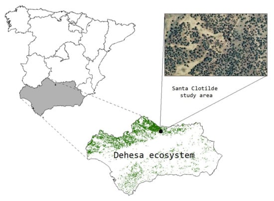
Figure 1.
Distribution of dehesa in Andalucia region (Spain) and the experimental area Santa Clotilde.
2.3. Remote Sensing Data Used to Derive TSEB Parameters (Soil and Plant Properties)
Two satellite sensors with different spatial and temporal resolutions were used as a source of surface radiometric temperature (TRAD) values: MODIS (Moderate Resolution Imaging Spectroradiometer) and Landsat 7ETM+ and 8OLI.
2.3.1. MODIS Data
MODIS sensor has daily coverage, with 250 m and 1 km spatial resolution for the visible and the thermal bands, respectively. The thermal product MYD11A1, which supplies TRAD with the atmospheric and emissivity effects corrected was used. For Las Majadas, 40 days in 2008 and 2011 were analyzed, and for Santa Clotilde site 65 days were used between 2012 and 2014. The dates used in the analysis have been selected from the data series from both ECT systems, discarding days according to the following criteria: (a) periods with gaps due to instrument failure; (b) lacking satellite thermal imagery over the ECT site due to clouds; and (c) unsuitable flux footprint due to wind direction. The selection was made to capture the seasonal variability of dehesa. However, in Santa Clotilde, the first data series collected by the ECT had several gaps, mainly due to the set-up and different tests performed on the tower and the instruments, and it was not always possible to capture an image every month. Nevertheless, the data collected was distributed as homogeneously as possible considering these limitations. For the derivation of the leaf area index and the fractional cover, red and near infrared (NIR) bands were used, as well as blue band for the green fraction, following the same procedure as described in the previous paper I [3].
When the MODIS satellite was used, the NDVI for the first period (2012 and part of 2013) over Santa Clotilde was derived from the separate Red and NIR bands daily reflectance data. For the following periods and for Las Majadas, after testing, the behavior of the MODIS product MOD13Q1 with 250 m resolution and 15-day frequency was regarded as accurate enough for our requirements. This product gives a NDVI value representative of the 15-day period, as the average of the two days with maximum NDVI and higher-quality information. Therefore, MOD13Q1 data are always slightly higher than daily derived NDVI from Red and NIR bands. However, since the RMSD = 0.03 between the estimated NDVI and that provided by MOD13Q1 product, yielding a relative error of 6% and a very similar temporal change, it was decided to use the MOD13Q1 product directly, facilitating the process.
● Derivation of oak LAI and total ecosystem LAI
To isolate the effect of the tree layer from the understory component and to study its variability during the year, the local LAI of the trees was derived from MODIS data for both locations, taking into account that the LAI index derived integrates the clumping effect. This was done for the period when the herbaceous layer was dry, assuming that the reflectance registered by the sensor corresponded only to the oaks. The estimated oak LAI results from Santa Clotilde were compared with field measurements of LAI to study the accuracy of the estimation. Local leaf area index measurements were made over the field using a linear Ceptometer AccuPAR (model LP-80, Decagon Devices) following the distribution of the ecosystem, integrating the relatively constant oak LAI along with the herbaceous layer LAI, with high seasonal variation. Only measurements on clear days, without cloud coverage and at nadir solar position (about 12 h GTM) were made. Seven days were analyzed following this procedure (21 June 2013, 23 July 2013 and 23 August 2013, 4 June 2014, 17 June 2014, 30 June 2014 and 17 July 2014). During the period with an active grass layer, with local LAI field measurements of both oaks and grass, an “average ecosystem LAI” weighted by the surface occupied by each component was derived and then compared with the MODIS-estimated index. Dates available for the analysis were 15 May 2013, 21 May 2013, 8 April 2013, 20 September 2013, 17 October 2013, 31 October 2013, 14 November 2013, 25 April 2014, and 19 May 2014.
Instantaneous energy fluxes were computed with MODIS data, as well as daily ET values for both study sites as described below and compared with the measurements of the two ECT systems. Distributed ET over Andalusian dehesa was also mapped using MODIS imagery, for monitoring the temporal and spatial condition of ecosystem health across the region.
● Daily evapotranspiration estimation
An integrated value of the latent heat flux over the day is more useful for agriculture and hydrological applications than the instantaneous values provided by the energy balance models at the time of the satellite overpass. Several extrapolation approaches have been proposed by different authors [23,24,25]. One of the most generalized solutions assumes that the energy partition among the balance components, expressed by the evaporative fraction (Fevap), remains constant over the day [23,26]. However, some authors [23,27,28] have found that the Fevap calculated in mid-days hours produced an underestimate of ET, because Fevap daily-curve has a convex shape with a minimum around noon. Differences of around 10% between estimated and daily fluxes for instantaneous values were found by Anderson et al., [29], computed at around the Landsat overpass time. For the same time of day, an optimal adjustment using measured fluxes with a correction coefficient of 1.1 was found by González-Dugo et al., [30]. We used an evaporative fraction given by:
to estimate the daily evapotranspiration integrating MODIS data into TSEB.
● Distributed evaluation of energy fluxes over Andalusian dehesas
For the application of the model to the entire Andalusian dehesa region, we selected 10 MODIS images from 2014 (2 February, 6 March, 21 March, 7 April, 30 April, 25 May 9 June, 26 June, 9 July and 17 July) with the lowest cloud coverage and distributed over the winter, spring and summer seasons. Meteorological variables used as model input, including air temperature and humidity, wind speed and solar incoming radiation were spatially interpolated with the inverse of distance algorithms, using half hourly data registered by 29 meteorological stations in the regional agroclimatic network (RIA). The stations were selected to integrate the variability between the different areas of dehesa to capture the heterogeneity in meteorological conditions within the Andalusian region.
Because the fluxes from the dehesa need to be estimated above the woodland turbulent layer, the spatial meteorological information must be measured at greater heights than usual (2 m), and the meteorological variables should be interpolated within the atmospheric surface layer until a height were the fluxes will be representative (~17 m). Under near-neutral atmospheric conditions extrapolating the wind speed, air temperature and humidity using a logarithmic profile up to ~20 m is considered reasonable. However, under highly stable or unstable conditions the logarithmic profile is significantly altered. Such conditions can occur: (a) when the vertical motion of air is suppressed by thermal stratification (stable condition), a situation that typically occurs at night when sensible heat (H) is negative (TA > TRAD); and (b) when H is positive (the surface is warmer than the air) and mixing is enhanced (unstable condition). In this study, unstable conditions are much more likely due to the daytime application of TSEB (~13:00 local time), determined by the satellite overpass time. These unstable conditions tend to create a more uniform wind profile than under neutral conditions, due to enhanced buoyancy resulting in strong vertical air motions suppressing a logarithmic wind speed profile.
The parameters used to estimate atmospheric stability usually require measurements of heat and momentum fluxes, or temperature at two different levels [31], not offered by the regional meteorological stations. Because temperature and velocity at only one height above the surface were available, bulk Richardson number was computed as the stability parameter (Rib values for near neutral conditions were considered to range between −0.005 to 0), being defined as:
where g is the acceleration of gravity, z is the height of the lowest level of the data, z0 is the roughness height, Δ (z − z0) is the difference in potential temperatures at z and z0, and u(z) is the wind speed at height z [32,33,34]. Approximate relationships between Monin–Obukhov stability parameter ζ (z/L), and Rib for stable and unstable surfaces layer were used to obtain Monin–Obukhov length (L) [34]. The atmospheric stability functions for heat and momentum transfer were then estimate, as wind-speed and temperature extrapolated to 17 m. The stations were located over bare soil and/or short grass (hC < 0.2 m) and the roughness length and zero-displacement height were taken equal to 1/8 hC and 2/3 hC, respectively.
2.3.2. Landsat Data
Eleven cloudless Landsat 7ETM + & 8OLI images (path 201 and row 33) coincident with the study period and the series of data from the Santa Clotilde ECT without gaps were also acquired and processed (DOY 124 for 2012 and 110, 182, 190, 198, 206, 214, 310, 318, 342, and 350 for 2013). The images were already geo-referenced, with spatial resolutions of 30 m in the shortwave bands and 60/100 m in the thermal band, depending on whether the satellite was 7ETM+ or 8OLI. Atmospheric and surface emissivity effects were corrected by an atmospheric radiative transfer model MODTRAN4 [35]. The lack of available atmospheric data required for an in-situ atmospheric characterization led us to use MODIS satellite-derived atmospheric profiles of air temperature and humidity (MOD07 product) which, according to [36], provides an RMSE of 0.6 K in radiometric temperature estimates compared to locally measured profiles. Landsat-7 ETM+ suffered a technical problem on 31 May 2003, related to the scan-line corrector, since when it has been operating without this instrument functioning properly. In this case, Santa Clotilde is on the east part of the image, with losses in pixels due to this effect that were visible in the results. No gap-filling technique was used. The same criteria as for MODIS data were used to select the images analyzed, and the footprint was computed for each day and time of the Landsat image selected.
● Footprint analysis
To validate the model estimates, it is necessary to determine the area which is contributing to the ECT measurements. As shown in [3], it is possible to integrate information from low spatial resolution sensors (pixel size ~103 m) directly along the principal component of the wind direction, due to the homogeneity in land cover. For Landsat, satellites, with medium spatial resolution (thermal pixel size of 60 and 100 m, respectively, for Landsat 7TM and Landsat 8OLI), a weighted integration of the pixels inside the contributing area was calculated, to validate these estimates against ground-truth measurements. The method used to calculate the footprint was described by Timmermans et al., [37].
A three-dimensional footprint model that calculates the source strength, Fx′y′, of a single observation point was used as follows:
where αy′ is the cross-wind spread in the direction y′ perpendicular to the wind direction (x′) and Fx′ is the relative contribution per running meter along the wind direction, as:
where kvk is the von Karman constant and zm the measuring height. The footprint model, described in detail in [38], was then combined with a weighting function to obtain the relative contribution of each pixel to the tower measurements. For the net radiation sensor, 99% of the observations originate from a circle whose diameter is ~12 times the sensor height (~210 m). However, since a re-sampling of the TRAD images to 30 m resolution of the visible bands, a fetch comprising 7 × 7 pixels of model output was taken in the upwind direction, and was used to accommodate the associated heterogeneity at this finer scale.
3. Results and Discussion
3.1. MODIS
3.1.1. Comparison between Estimated and Measured LAI
The RMSD between ground-based estimated and remotely-sensed local oak LAI values for Santa Clotilde was 0.12, which yielded an error of around 15% (Figure 2). For the average LAI of the complete ecosystem (grass + oak trees), taking into account the changes in the pasture layer, the RMSD was 0.45, which yielded 30% of error. As we can see in Figure 2, the measured ecosystem LAI was in general lower than the remotely-sensed value (overestimation of ecosystem LAI). This could be caused by a scale mismatch between the ground observations and the remotely sensed estimates. Constant values of oak and grass ground fraction coverage were assumed for every day having ground measurements, with the effect of the bare soil integrated into the grass measurements. During the study period (2012–2014 for Santa Clotilde and 2008–2011 for Las Majadas), the mean MODIS estimated local LAI for the oaks (integrating a constant 0.2 fC for the trees and estimated during summer) over Santa Clotilde was 3.17, with a standard deviation of 0.09, 3.37 over Las Majadas with similar σ value. The variability of the local LAI for the oaks estimated with MODIS during the year is slightly higher. Effective total LAI values of 1.06 (σ = 0.65) and 1.26 (σ = 0.49) were estimated for Santa Clotilde and Las Majadas, respectively, with higher deviation than oak LAI, caused by the grass influence.
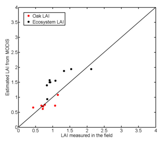
Figure 2.
Comparison between effective LAI observed in the field (following the ecosystem structure with a constant fc for trees and grasses) and MODIS-estimated LAI for Santa Clotilde.
3.1.2. Distributed Application Using MODIS Images over Las Majadas and Santa Clotilde
The TSEB model was applied and evaluated over both areas, finding that the Root Mean Square Difference (RMSD) values for the energy fluxes (Table 1) are within the range found by other authors [5,30,39,40,41] and consistent with typical uncertainties derived for the flux measurement system (~40 W m−2) (e.g., [42]). The energy closure errors for Santa Clotilde were evaluated for the study period, yielding average closures of 80% for Santa Clotilde and 86% for Las Majadas, representing 49 Wm−2 and 40 Wm−2 respectively. In a similar sparse, semi-arid ecosystem (olive orchard) as the dehesa, RMSD values were found for Rn of 28 Wm−2, for G of 17 Wm−2, and 40 and 43 Wm−2 for H and LE, respectively [16]. It can be derived from the comparison with [16] results, that an important source of error might be the higher soil heat flux error found in the dehesa application, as this directly influences the available energy of the system. In a much more arid environment (almost a desert) RMSD values were found for Rn of 58 Wm−2, 64 Wm−2 for H and 105 for LE Wm−2, with canopy and soil radiometric temperatures ground data [43]. In Kustas et al., [44], a revision of Morillas et al., [43] data analysis was done, confirming the results but significantly reducing the bias using key vegetation inputs to TSEB, and a modification of the soil resistance formulation.

Table 1.
TSEB-MODIS RMSD of the surface energy fluxes for Las Majadas and Santa Clotilde.
LE relative error increases during the summer, due to the low rates of the daily flux over this semi-arid ecosystem. Differences in the Rn and turbulent fluxes magnitudes (Figure 3 and Figure 4) between both locations are due to the different periods/seasons selected. At Santa Clotilde (Figure 3), many days during the dry summer period were analyzed, with LE values being more concentrated and less dispersed than at Las Majadas (Figure 4).
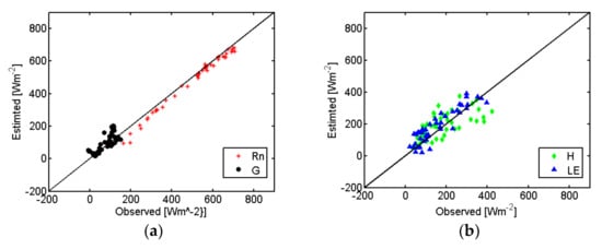
Figure 3.
TSEB-MODIS estimated values and ECT observed values of energy fluxes over Las Majadas site during 2008 and 2011. (a) Solar net radiation (Rn) and soil heat flux (G), (b) Sensible heat flux (H) and latent heat flux (LE).
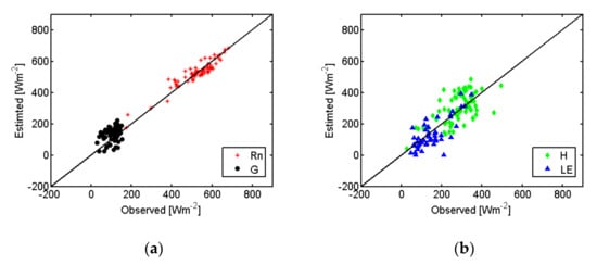
Figure 4.
TSEB-MODIS estimated values and ECT observed values of energy fluxes over Santa Clotilde site during 2012–2014. (a) Solar net radiation (Rn) and soil heat flux (G), (b) Sensible heat flux (H) and latent heat flux (LE).
3.1.3. Daily ET Temporal Evaluation
Daily estimations of ET integrating MODIS data (Figure 5) were compared to the ground-truth measurements yielding a RMSD of 1 mm day−1 for Las Majadas and 0.9 mm day−1 for Santa Clotilde. Although the extrapolation to daily ET using 1.1 Fevap (Equation (3)) during the day might contribute to the discrepancies of estimated and observed values, this accuracy was regarded as being good enough for management purposes and similar to values found by other authors for more homogeneous crops [45] and similar woody sparse semi-arid crops as vineyards [46]. However, further research of the Fevap daily-curve of this particular ecosystem (i.e., analyzing Fevap with ECTs data) is needed, particularly during stress conditions [27]. These results are also within the range of previous studies of this system using a different approach based on water balance and vegetation index-derived crop coefficients, where a RMSD was found for daily ET of 0.55 mm day−1, but required calibration [47]. This agreement may encourage further studies to integrate the water balance with the TSEB ET estimates taking advantage of the utility of both methodologies.
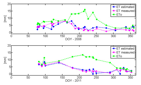
Figure 5.
TSEB-MODIS daily estimated ET and daily measured ET (ECTs) and ET0 for Las Majadas (2008 and 2011).
Daily ET data derived from remote sensing allow the ecosystem to be monitored on a constant basis, and thus enable the degree of vegetation water stress to be assessed by comparing actual with potential ET values. Figure 5 shows how, in Las Majadas (2008) after the end of June (around DOY 175), the curves of actual ET and reference ET (ETO) display opposing trends, which means that the transpiration rate is drastically reduced during the summer. This is due to the senescence of the grass vegetation and the reduction of oak transpiration caused by soil water deficit in the root zone. The stressed condition occurred when the evaporative demand exceeded the capability of the vegetation to access available water.
Although days with data points are linearly connected in Figure 5 to illustrate the evolution of ET values, the interpolation between dates is not likely to be linear due to sharp changes due to rainfall or other weather related conditions (cloud cover, vapor pressure, air temperature and wind). This limitation can be overcome to some extent using daily MODIS data, which can provide more frequent surface radiometric temperature data, depending on the cloud coverage. When the temporal resolution of the satellites or cloud coverage does not permit continuous monitoring, the coupling between water and energy balance models might present a good solution, using the information derived from the TSEB as a real proxy of the ecosystem water status to be incorporated in the continuous water-balance approach.
3.1.4. Analysis of Distributed Instantaneous Energy Fluxes over Andalusian Dehesas
For this first attempt to evaluate the energy fluxes over Andalusian dehesas, 10 days from 2014 within winter, spring and summer were selected and analyzed, with the objective of evaluating a future extension of the study using daily MODIS images, depending on the cloud cover. Distributed maps of meteorological variables (Figure 6) were used as input to study the heterogeneity of the region, where the differences in orographic, meteorological, abiotic and biotic conditions create different Mediterranean subtypes (bioclimatic levels). The fractional coverage of the vegetation of the entire region is also shown for the wet and dry seasons (Figure 7), and we can observe the differences between zones caused by climate and land use variability. The densest coverages are located over the natural parks in the Cádiz region (Zone 1) and lower coverages over the north of Andalucía (Zone 2). In the Cardeña y Montoro natural park (Zone 3) the mean values of fC are shown. We selected these zones as examples to provide some insights in the behavior of surface energy fluxes throughout the year.
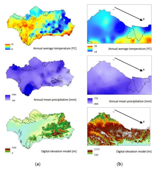
Figure 6.
Annual mean values for temperature and precipitation for: (a) the entire Andalusian region; and (b) Zones 2 and 3.
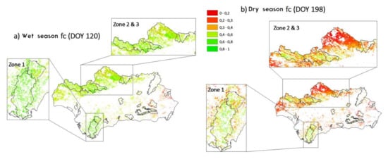
Figure 7.
MODIS-estimated fractional cover for Andalusian dehesa for the: (a) wet season; and (b) dry season. Other land-uses different from dehesa were masked (white area).
The densest forested areas are located over zones with higher annual mean precipitation and a moderate Mediterranean climate, due to the proximity to the sea that reduces annual temperature oscillations (Figure 6). The mountains of Grazalema and Los Alcornocales natural parks offer a topographic wall to the Atlantic ocean’s water-saturated winds. As a result, rainfall events are very intense, with some points registering the highest rates in Spain with more than 2200 mm per year. (Figure 6). Due to the differences in these conditions compared to other areas of dehesa, other species occur more frequently than Quercus ilex; these include Quercus suber and Quercus faginea, and to a lesser extent Quercus pyrenaica. The variety of wild olive tree, commonly known as acebuche (Olea europaea var. sylvestris), is also widely distributed throughout all dehesa ecosystems. During the dry season when the sub-canopy layer is not active, the fractional cover values derived from the remotely sensed information are due only to the oaks. In Figure 7, we can see that fC = 0.2 for almost the entire dehesa area except Zone 1, where woodlands are dense. As Figure 6 shows, between Zones 2 and 3 there is a rising gradient in precipitation and air temperature, in southwesterly direction, that results in the different canopy and soil conditions.
Stability effects may be an important source of error for these large-scale estimates when strongly unstable or stable conditions are observed, and the logarithmic profile assumption is tenuous. The area with higher unstable conditions is Zone 2. Zone 1 has more near-neutral conditions, with high wind speed values frequently recorded.
As expected, during the dry season (Figure 8), LE showed the lowest values, due to water scarcity and the summer meteorological conditions. Nevertheless, over Zone 1 (Figure 8), it was still possible to observe relatively high values of this flux (~300 W m−2), due to the unique meteorological characteristics of this region. Higher water availability conditions may be ascribed to summer fogs and mists, known as “barbas de levante”, moisturizing the environment. The strong winds of the area, due to the proximity of the Strait of Gibraltar and the topography of the mountains, have similar effects, bringing humidity from the sea. These factors create a special micro-climate similar to subtropical areas [48]. Throughout the year, the dehesa located in Zone 2 displayed the lowest values of ET, due to the low annual mean precipitation together with a strongly arid climate and low vegetation fractional cover. In these areas, it is likely that one of the canopy mechanisms that enable dehesa to adapt to the harsh environment conditions is reducing the ecosystem fractional cover, as we can see in Figure 7. The H, Rn and G showed lower values during the winter, as expected, and higher values during the dry season, when the surface temperature significantly increased.
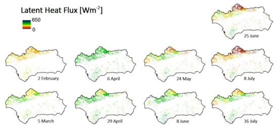
Figure 8.
TSEB-MODIS estimated LE distributed over Andalusian dehesa for 2014. Other land-uses different from dehesa were masked (white area).
3.2. Distributed Application Using Landsat 7 ETM+ and 8 OLI Images over Santa Clotilde
Energy fluxes estimations at higher spatial resolution better capture the heterogeneity of the area, required for rangeland planning at local scale, such us cattle density, water reservoirs and vulnerable areas management. It also allows for the validation with field ground data. To compare the turbulent fluxes results with the measurements it is necessary to weight the pixels that contribute to the ECT measurements. In this case, the footprint analysis was made following the procedure described by Timmermans et al., [37]. On 80% of the days analyzed using Landsat images, the wind direction corresponded to the predominant one (southwest, SW). A high wind speed also means a larger footprint, and this needs to be incorporated in the validation. After studying the homogeneity of the area when no predominant wind direction was observed, we selected the days where a comparison with the ECT measurements was possible. Results showed a RMSD of 64 Wm−2 for LE (38% absolute difference), 51 Wm−2 for H (26% absolute difference), and 44 (7%) and 40 (36%) Wm−2 for Rn and G respectively, somewhat higher than the errors found for the MODIS application but still within a similar range. Absolute discrepancies applying the model with the radiometric temperature derived from the four-way radiometer over the same areas [3] showed slightly higher values than the distributed application, particularly for Rn and G. This result, an increase in the error while the spatial resolution is refined, might be due to the average TRAD provided by the satellite, which better integrates the heterogeneity of the source area measured by the ECT. Estimates of the G as a function of Rn reaching the soil and the time of the day may be not adequately modeled. Even when it integrates the seasonal variation of net radiation over the year, the ratio between G/Rn might not be the same during dry versus wet period [39]. Due to the deployment of the sensors measuring G in the field, being located inside two enclosures for protecting sensors from animals (sensors installed under a tree-EA1 and on the open grass-EA2), the measurements might be not representative of the surrounding areas. The partition between the net radiation reaching the soil and the vegetation, influenced by the two different layers of canopy (i.e., understory vegetation) might not be accurately estimated for this type of ecosystem.
Figure 9 shows an example of the distributed fluxes estimated over Santa Clotilde. Results derived from Landsat-7 ETM+ TRAD images include the scan lines with no data. The heterogeneity of the area is better portrait using higher spatial resolution images, where it is possible to observe (Figure 9) the different features of the environment, and to distinguish between highly vegetated and bare soil, or dryer and wetter areas. Depending on the final use of the information (e.g., regional drought evaluation vs. farming seasonal planning) different spatial and temporal resolutions will be necessary. In the case of local applications medium and high spatial resolution are required. Therefore, the accuracy of the TSEB application integrating Landsat images over dehesa is promising for rangeland management purposes. It can be seen that in summer H over the area is high compared to LE, and the trend is opposite during wet periods (typically in May) with maximum values of LE, as expected. However, during the winter, both turbulent fluxes are low, probably due to the low values of available energy and the lack of precipitation during the days studied. Spatial quantification of these variables, together with their evolution under different circumstances, in the context of climate change effects such as droughts, water logging or heat waves, could help to monitor the functioning of the ecosystem and its response to these extreme events.
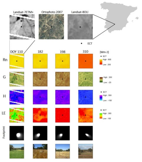
Figure 9.
TSEB-Landsat energy fluxes distributed estimations for Santa Clotilde experimental site for 2013.
4. Conclusions
Mapping ET on a regional scale is possible by integrating earth observations and spatially-distributed meteorological data into the TSEB model, providing a better representation of the heterogeneity in land cover and local meteorological conditions. Instantaneous LE values and the associated daily ET values are derived using MODIS images, with 1 km spatial resolution and daily temporal frequency (depending on the cloud cover) for both study sites (Las Majadas and Santa Clotilde). The difference between estimated and observed surface fluxes are consistent with typical uncertainties derived for ECT measurement systems, being sufficiently accurate to be employed in a distributed way and on a more regular basis. TSEB is also evaluated using a higher spatial resolution satellite (30/100 m), Landsat-7 ETM+ and Landsat-8 OLI for the Santa Clotilde site with similar accuracy. The heterogeneity of the experimental area is a better portrayed following this approach. For local rangeland management purposes, medium and high spatial resolutions are required, being these results promising for the development of a local monitoring tool for decision-making.
An important source of error could be due to the measurement and modeling of G. The soil heat flux directly influences the system (soil/grass understory + oak tree overstory) available energy, limiting the energy for latent and sensible heat fluxes. However, this flux is difficult to measure over the landscape, due to the heterogeneity of the experimental areas and the difficulties involved in distributing sensors across the fetch of the tower measurements, due to the extensive livestock grazing that is typical in the region. Discrepancies between observed and estimated fluxes might also be due to the sub-canopy layer existence, with a different phenology and physiology than that of the oaks. These aspects require further research, and an attempt should be done to integrate the different layers into the radiation and surface energy budgets. Discrepancies applying the model with the radiometric temperature derived from the four-way radiometer over the same areas [3], followed by the Landsat application, showed slightly higher values than the distributed application using MODIS, particularly for net radiation and soil heat flux. This improvement on the accuracy while the spatial resolution is reduced, might be due to the average TRAD provided by the satellite, which better integrates the heterogeneity of the source area measured by the ECT.
Distributed LE over Andalusian dehesa is mapped as a first approach to monitor the ecosystem status on a regular basis, with the objective of assessing the applicability of satellites together with a meteorological network, used in a remote sensing-based energy balance model (TSEB). It is shown that it is possible to derive reliable LE/ET values that reflect the local conditions and micro-climates, and the evolution of the vegetation cover over all the seasons. The gaps caused by the existence of clouds might be solved in a future by coupling these remote sensing energy balance techniques with water balance approaches, together with the use of various satellites with different spatial and temporal resolutions. The application of meteorological forcing data from a network of weather stations requires assumptions about variability in meteorological conditions, as well as a technique for extrapolation of wind and air temperature profiles to represent conditions above tall canopies. Instead, either using the Atmospheric Land Exchange Inverse (ALEXI) model, which prescribes the air temperature at nominally 50 m above the land surface [49], or using MODIS atmospheric temperature and moisture profiles (atmospheric stability product [50]) removes the need for these observations, being dependent on local conditions.
Acknowledgments
We would like to thank the owners and workers of Santa Clotilde experimental site, as well as Arnaud Carrara and the group managing the experimental site of Las Majadas for the ground-truth ECT measurements and the additional data. This work has been funded by the Andalusian Institute for Agricultural and Fisheries Research and Training (IFAPA, Consejería de Agricultura, Pesca y Desarrollo Rural de la Junta de Andalucía) and the European Social Fund Operational Programme 2007–2013, in the field of priority Axis 3 (Improving human capital), in an 80%. This project has also received funding from the European Union’s Horizon 2020 Research and Innovation programme under the Marie Skłodowska-Curie grant agreement No. 703978, and INIA-FEDER 2014-2020 (Operational Programme Smart Growth) project RTA2014-00063-C04-02.
Author Contributions
A.A. and M.P.G.-D. conceived and designed the experiments; A.A. performed the experiments, analyzed the data and wrote the paper; W.P.K. contributed to the interpretation of data and designed of the experiments; and A.C. and M.J.P. reviewed the paper.
Conflicts of Interest
The authors declare no conflict of interest. The founding sponsors had no role in the design of the study; in the collection, analyses, or interpretation of data; in the writing of the manuscript, and in the decision to publish the results.
References
- Martin Bellido, M. La dehesa. Agricultura 1996, 762, 44–49. [Google Scholar]
- Pulido, F.J.; Díaz, M. Regeneration of a Mediterranean oak: A whole-cycle approach. Ecoscience 2016, 12, 92–102. [Google Scholar] [CrossRef]
- Andreu, A.; Kustas, W.P.; Polo, M.J.; Carrara, A.; Gonzalez-Dugo, M.P. Modelling surface energy fluxes over a dehesa (oak savanna) ecosystem using a thermal based Two-Source Energy Balance model (TSEB) I. Remote Sens. 2018, in press. [Google Scholar]
- Moran, S. Thermal Infrared Measurement as an Indicator of Plant Ecosystem Health. In Thermal Remote Sensing in Land Surface Processes; Taylor & Francis: New York, NY, USA, 2004; pp. 257–282. ISBN 0-415-30224-2. [Google Scholar]
- Kustas, W.P.; Norman, J.M. Evaluation of soil and vegetation heat flux predictions using a simple two-source model with radiometric temperatures for partial canopy cover. Agric. For. Meteorol. 1999, 94, 13–29. [Google Scholar] [CrossRef]
- Li, F.; Kustas, W.P.; Prueger, J.H.; Neale, C.M.U.; Jackson, T.J. Utility of remote sensing–based Two-Source Energy Balance Model under low- and high-vegetation cover conditions. J. Hydrometeorol. 2005, 6, 878–891. [Google Scholar] [CrossRef]
- Kustas, W.P.; Norman, J.M. A Two-Ssource approach for estimating turbulent fluxes using multiple angle thermal infrared observations. Water Resour. Res. 1997, 33, 1495–1508. [Google Scholar] [CrossRef]
- Choudhury, B.J. Relationships between vegetation indices, radiation absorption, and net photosynthesis evaluated by a sensitivity analysis. Remote Sens. Environ. 1987, 22, 209–233. [Google Scholar] [CrossRef]
- Campbell, G.S.; Norman, J.M. An Introduction to Environmental Biophysics; Springer: Delhi, India, 2009; ISBN 978-0-387-94937-6. [Google Scholar]
- Kustas, W.P.; Norman, J.M. A Two-Source Energy Balance Approach Using Directional Radiometric Temperature Observations for Sparse Canopy Covered Surfaces. Agron. J. 2000, 92, 847–854. [Google Scholar] [CrossRef]
- Ross, J. Radiative transfer in plant communities. In Vegetation and the Atmosphere; Monteith, J.L., Ed.; Academic Press: London, UK, 1975; Volume 1, pp. 13–55. [Google Scholar]
- Lhomme, J.-P.; Chehbouni, A. Comments on dual-source vegetation–atmosphere transfer models. Agric. For. Meteorol. 1999, 94, 269–273. [Google Scholar] [CrossRef]
- Kustas, W.P.; Daughtry, C.S. Estimation of the soil heat flux/net radiation ratio from spectral data. Agric. For. Meteorol. 1990, 49, 205–223. [Google Scholar] [CrossRef]
- Friedl, M.A. Relationships among remotely sensed data, surface energy balance, and area-averaged fluxes over partially vegetated land surfaces. J. Appl. Meteorol. 1996, 35, 2091–2103. [Google Scholar] [CrossRef]
- Cellier, P.; Richard, G.; Robin, P. Partition of sensible heat fluxes into bare soil and the atmosphere. Agric. For. Meteorol. 1996, 82, 245–265. [Google Scholar] [CrossRef]
- Cammalleri, C.; Anderson, M.C.; Ciraolo, G.; D’Urso, G.; Kustas, W.P.; La Loggia, G.; Minacapilli, M. The impact of in-canopy wind profile formulations on heat flux estimation in an open orchard using the remote sensing-based two-source model. Hydrol. Earth Syst. Sci. 2010, 14, 2643–2659. [Google Scholar] [CrossRef]
- Brutsaert, W. Evaporation into the Atmosphere: Theory, History and Applications; Kluwer: Dordrecht, The Netherlands, 2010. [Google Scholar]
- Priestley, C.H.B.; Taylor, R.J. On the assessment of surface heat flux and evaporation using large-scale parameters. Mon. Weather Rev. 1972, 100, 81–92. [Google Scholar] [CrossRef]
- Carreiras, J.; Pereira, J.M.C.; Pereira, J.S. Estimation of tree canopy cover in evergreen oak woodlands using remote sensing. For. Ecol. Manag. 2006, 223, 45–53. [Google Scholar] [CrossRef]
- Foken, T. The energy balance closure problem: An overview. Ecol. Appl. 2008, 18, 1351–1367. [Google Scholar] [CrossRef] [PubMed]
- Franssen, H.J.H.; Stöckli, R.; Lehner, I.; Rotenberg, E.; Seneviratne, S.I. Energy balance closure of eddy-covariance data: A multisite analysis for European FLUXNET stations. Agric. For. Meteorol. 2010, 150, 1553–1567. [Google Scholar] [CrossRef]
- Schuepp, P.H.; Leclerc, M.Y.; MacPherson, J.I.; Desjardins, R.L. Footprint prediction of scalar fluxes from analytical solutions of the diffusion equation. Bound.-Layer Meteorol. 1990, 50, 355–373. [Google Scholar] [CrossRef]
- Crago, R.; Brutsaert, W. Daytime evaporation and the self-preservation of the evaporative fraction and the Bowen ratio. J. Hydrol. 1996, 178, 241–255. [Google Scholar] [CrossRef]
- Allen, R.G.; Morse, A.; Tasumi, M.; Trezza, R.; Bastiaanssen, W.G.M.; Wright, J.L.; Kramber, W. Evapotranspiration from a satellite-based surface energy balance for the Snake River Plan aquifer in Idaho. Proceeding of the USCID/EWRI Conference on Energy, Climate, Environment, and Water, San Luis Obispo, CA, USA, 9–12 July 2002; U.S. Committee on Irrigation and Drainage: Denver, CO, USA, 2002. [Google Scholar]
- Jackson, R.D.; Hatfield, J.L.; Reginato, R.J.; Idso, S.B.; Pinter, P.J. Estimation of daily evapotranspiration from one-time-of-day measurement. Agric. Water Manag. 1983, 7, 351–362. [Google Scholar] [CrossRef]
- Shuttleworth, W.J.; Gurney, R.J.; Hsu, A.Y.; Ormsby, J.P. FIFE: The variation in energy partition at surface flux sites. In Remote Sensing and Large-Scale Processes, Proceedings of the IAHS Third International Assembly; Rango, A., Ed.; IAHS Publication: Baltimore, MD, USA, 1989; Volume 186, pp. 67–74. [Google Scholar]
- Lhomme, J.-P.; Elguero, E. Examination of evaporative fraction diurnal behaviour using a soil-vegetation model coupled with a mixed-layer model. Hydrol. Earth Syst. Sci. 1999, 3, 259–270. [Google Scholar] [CrossRef]
- Gentine, P.; Entekhabi, D.; Chehbouni, A.; Boulet, G.; Duchemin, B. Analysis of evaporative fraction diurnal behavior. Agric. For. Meteorol. 2007, 143, 13–29. [Google Scholar] [CrossRef]
- Anderson, M.C.; Norman, J.M.; Diak, G.R.; Kustas, W.P.; Mecikalski, J.R. A two-source time-integrated model for estimating surface fluxes using thermal infrared remote sensing. Remote Sens. Environ. 1997, 60, 195–216. [Google Scholar] [CrossRef]
- González-Dugo, M.P.; Neale, C.M.U.; Mateos, L.; Kustas, W.P.; Prueger, J.H.; Anderson, M.C.; Li, F. A comparison of operational remote sensing-based models for estimating crop evapotranspiration. Agric. For Meteorol. 2009, 149, 1843–1853. [Google Scholar] [CrossRef]
- Arya, S.P. Introduction to Micrometeorology; Academic Press: San Diego, CA, USA, 2009; ISBN 978-0-12-059354-5. [Google Scholar]
- Louis, J.-F. A Parametric Model of Vertical Eddy Fluxes in the Atmosphere. Bound.-Layer Meteorol. 1979, 17, 187–202. [Google Scholar] [CrossRef]
- Delage, Y. A parameterization of the stable atmospheric boundary layer. Bound.-Layer Meteorol. 1988, 43, 365–381. [Google Scholar] [CrossRef]
- Byun, D.W. On the analytical solutions of flux-profile relationships for the atmospheric surface layer. J. Appl. Meteorol. 1990, 29, 652–657. [Google Scholar] [CrossRef]
- Berk, A.; Bernstein, L.S.; Anderson, G.P.; Acharya, P.K.; Robertson, D.C.; Chetwynd, J.H.; Adler-Golden, S.M. MODTRAN Cloud and multiple scattering upgrades with application to AVIRIS. Remote Sens. Environ. 1998, 65, 367–375. [Google Scholar] [CrossRef]
- Jimenez-Muñoz, J.C.; Sobrino, J.A.; Mattar, C.; Franch, B. Atmospheric correction of optical imagery from MODIS and Reanalysis atmospheric products. Remote Sens. Environ. 2010, 114, 2195–2210. [Google Scholar] [CrossRef]
- Timmermans, W.J.; Su, B.; Olioso, A. Footprint issues in scintillometry over heterogeneous landscapes. Hydrol. Earth Syst. Sci. 2009, 13, 2179–2190. [Google Scholar] [CrossRef]
- Soegaard, H.; Jensen, N.O.; Boegh, E.; Hasager, C.B.; Schelde, K.; Thomsen, A. Carbon dioxide exchange over agricultural landscape using eddy correlation and footprint modelling. Agric. For. Meteorol. 2003, 114, 153–173. [Google Scholar] [CrossRef]
- Norman, J.M.; Kustas, W.P.; Humes, K.S. Source approach for estimating soil and vegetation energy fluxes in observations of directional radiometric surface temperature. Agric. For. Meteorol. 1995, 77, 263–293. [Google Scholar] [CrossRef]
- Timmermans, W.J.; Kustas, W.P.; Anderson, M.C.; French, A.N. An intercomparison of the Surface Energy Balance Algorithm for Land (SEBAL) and the Two-Source Energy Balance (TSEB) modeling schemes. Remote Sens. Environ. 2007, 108, 369–384. [Google Scholar] [CrossRef]
- Sanchez, J.M.; Kustas, W.P.; Anderson, M.C.; Caselles, V. Modelling surface energy fluxes over maize using a two-source patch model and radiometric soil and canopy temperature observations. Remote Sens. Environ. 2008, 112, 1130–1143. [Google Scholar] [CrossRef]
- Twine, T.E.; Kustas, W.P.; Norman, J.M.; Cook, D.R.; Houser, P.R.; Meyers, T.P.; Prueger, J.H.; Starks, P.J.; Wesely, M.L. Correcting eddy-covariance flux underestimates over a grassland. Agric. For. Meteorol. 2000, 103, 279–300. [Google Scholar] [CrossRef]
- Morillas, L.; Garcia, M.; Nieto, H.; Villagarcia, L.; Sandholt, I.; Gonzalez-Dugo, M.P.; Zarco-Tejada, P.J.; Domingo, F. Using radiometric surface temperature for surface energy flux estimation in Mediterranean drylands from a two-source perspective. Remote Sens. Environ. 2013, 136, 234–246. [Google Scholar] [CrossRef]
- Kustas, W.P.; Anderson, M.C.; Alfieri, J.G.; Nieto, H.; Morillas, L.; Hipps, L.E.; Villagarcia, L.; Domingo, F.; Garcia, M.; Garcia, M. Revisiting the paper Using radiometric surface temperature for surface energy flux estimation in Mediterranean drylands from a two-source perspective. Remote Sens. Environ. 2016, 184, 645–653. [Google Scholar] [CrossRef]
- Kustas, W.P.; Anderson, M.C.; Cammalleri, C.; Alfieri, J.G. Utility of a thermal-based Two-source Energy Balance Model for estimating surface fluxes over complex landscapes. Procedia Environ. Sci. 2013, 19, 224–230. [Google Scholar] [CrossRef][Green Version]
- González-Dugo, M.P.; Escuin, S.; Cano, F.; Cifuentes, V.; Padilla, F.L.M.; Tirado, J.L.; Oyonarte, N.; Fernández, P.; Mateos, L. Monitoring evapotranspiration of irrigated crops using crop coefficients derived from time series of satellite images. II. Application on basin scale. Agric. Water Manag. 2013, 125, 92–104. [Google Scholar] [CrossRef]
- Campos, I.; Villodre, J.; Carrara, A.; Calera, A. Remote sensing-based soil water balance to estimate Mediterranean holm oak savanna (dehesa) evapotranspiration under water stress conditions. J. Hydrol. 2013, 494, 1–9. [Google Scholar] [CrossRef]
- Elías, F.; Ruiz, L. Agroclimatología de España; Ministerio de Agricultura, Instituto Nacional de Investigaciones Agrarias: Madrid, Spain, 1977.
- Anderson, M.; Kustas, W.P.; Norman, J.; Hain, C.; Mecikalski, J.; Schultz, L.; González-Dugo, M.; Cammalleri, C.; D’Urso, G.; Pimstein, A.; et al. Mapping daily evapotranspiration at field to global scales using geostationary and polar orbiting satellite imagery. Hydrol. Earth Syst. Sci. 2011, 15, 223–239. [Google Scholar] [CrossRef]
- Borbas, E. MODIS Atmosphere L2 Atmosphere Profile Product. NASA MODIS Adaptive Processing System; NASA, Goddard Space Flight Center: Greenbelt, MD, USA, 2015; Volume 1. [Google Scholar]
© 2018 by the authors. Licensee MDPI, Basel, Switzerland. This article is an open access article distributed under the terms and conditions of the Creative Commons Attribution (CC BY) license (http://creativecommons.org/licenses/by/4.0/).