Railway Track Condition Assessment at Network Level by Frequency Domain Analysis of GPR Data

Abstract

The railway track system is a crucial infrastructure for the transportation of people and goods in modern societies. With the increase in railway traffic, the availability of the track for monitoring and maintenance purposes is becoming significantly reduced. Therefore, continuous non-destructive monitoring tools for track diagnoses take on even greater importance. In this context, Ground Penetrating Radar (GPR) technique results yield valuable information on track condition, mainly in the identification of the degradation of its physical and mechanical characteristics caused by subsurface malfunctions. Nevertheless, the application of GPR to assess the ballast condition is a challenging task because the material electromagnetic properties are sensitive to both the ballast grading and water content. This work presents a novel approach, fast and practical for surveying and analysing long sections of transport infrastructure, based mainly on expedite frequency domain analysis of the GPR signal. Examples are presented with the identification of track events, ballast interventions and potential locations of malfunctions. The approach, developed to identify changes in the track infrastructure, allows for a user-friendly visualisation of the track condition, even for GPR non-professionals such as railways engineers, and may further be used to correlate with track geometric parameters. It aims to automatically detect sudden variations in the GPR signals, obtained with successive surveys over long stretches of railway lines, thus providing valuable information in asset management activities of infrastructure managers.

1. Introduction

Up to date information on the real condition of transport infrastructures is crucial for asset management activities, such as efficient maintenance and rehabilitation planning, and also to assess the performance and the service quality of the transport system.

Railway track condition assessment mainly consists of measuring parameters related to the rail wearing and positioning (track geometric quality). The main geometric parameters monitored are rail gauge, cant (cross level), cant gradient (twist), longitudinal level and longitudinal alignment, measured using dedicated inspection vehicles [1,2]. The others parameters, that are assessed to analyse the track condition, are the rail profile, rail roughness and its integrity; this last one is measured using ultrasounds [1]. Generally, during maintenance operations some track components are replaced while others remain the same, in particular the substructure [1,3]. For example, the normal causes of a rail longitudinal level defects (i.e., presence of ballast pockets, fouled ballast, poor drainage, subgrade settlements and transition problems) are therefore not detected by this monitoring procedure [4,5,6].

An important tool, increasingly used for railway monitoring, is Ground Penetrating Radar (GPR), which is a non-destructive testing (NDT) technique that provides an overall image of the subsurface [7]. This method allows operating with suspended antennas (air-coupled antennas), mounted on railway vehicles, and with high rates of data acquisition without disturbing the transport infrastructure, nor the normal traffic flow [8]. A GPR test can be carried out at different stages of the railway service life, from preliminary prospection to prepare the design of a new line, to quality control during construction [9,10], as well as to assess the causes of track geometry problems and to support maintenance planning decisions [2,11]. Nevertheless, GPR is not yet used in a systematic way for railway track characterisation and rehabilitation planning. The “traditional” way, in which the GPR signal is analysed, is still a more or less detailed interpretation of the signal in the time domain, generally performed in specific locations or for a particular purpose such as, for example, subgrade characterisation or fouling detection. These procedures are time consuming and require significant experience, being mainly undertaken by GPR professionals [2,12,13,14,15,16,17].

The method presented in this manuscript was developed for practical reasons, as a support tool to be used by the industry, namely to fulfil the Industry 4.0 ambitious objective to do an “almost live” diagnosis of the track [18,19]. The expedite macro-scale processing of GPR data proposed herein, enables continuous and efficient (although qualitative) survey and analysis of track condition. The approach contributes to promoting a wider use of GPR in railway area of application and represents a first step towards the development of quality indexes and alert levels for track network evaluation. GPR antennas can be installed in normal trains and used continuously along the year; it is therefore easy and not excessively expensive to upgrade railways networks by equipping a suitable number of trains with GPR instrumentation. The information acquired by GPR units can then be quickly processed by using the method proposed in this paper (and more advanced versions of it, to be developed in the future). Should be highlighted that the methodology developed in this study is not aimed to be used for detailed electromagnetic analysis of the GPR signal on tracks at limited locations, but rather in a preliminary stage of the GPR results analysis, at network level, to detect areas of the railway track that need a more thorough investigation to be done by using other signal processing techniques.

The approach presented in this study consists in analysing the GPR signals, in both time and frequency domains, to identify changes along significant lengths of railway line that can either correspond to known track singularities or to track pathologies. The processing focuses on specific time intervals and frequency ranges of the signal that are considered to be more representative for identifying changes in infrastructure along the track [15,17]. Four parameters were defined and implemented for track changes identification. A script was developed in MATLAB for GPR data processing that can be further integrated with track geometry data and aerial photography for a user-friendly interpretation.

The method allows three different levels of track assessment:

• diagnosis during inspection survey and detection of events and possible track defects;
• systematic events identification, in consecutive surveys, performed yearly in the same season;
• identification of track changes by comparing surveys performed in distinct climate condition along the year (e.g., summer vs. winter).

The latter differences might be caused by changes in water content due to poor drainage conditions or ballast fouling.

In Section 2, a review on the use of GPR for track assessment is provided, with special emphasis on the advantages of looking at data not only in the time domain but also in the spectral domain. In Section 3, the data processing method developed in this study is described and some examples are presented. In Section 4, the method is applied to a real-world case study; moreover, recommendations are suggested for combining GPR results with track geometry assessment for condition evaluation. Conclusions are presented in Section 5.

2. Ground Penetrating Radar for Track Assessment

2.1. Overview on the Use of GPR for Railway Monitoring

In recent years, there has been an increased interest in using NDT techniques for track evaluation in order to better characterise its behaviour. Apart from GPR, the main geophysical methods applied for railway monitoring are the Electric Resistivity Tomography (ERT), seismic and gravimetry [20,21,22,23,24]. A review on the geophysical methods generally used on railways is presented in [20]. For example, Falling Weight Deflectometer (FWD), Light FWD and prototype vehicles such as Rolling Stiffness Measurement Vehicle were used, at research level, to determine areas with low density, voids and damp [3,25,26]. In [21], a geophysical study is presented to evaluate the stability of railways combining 3D GPR, ERT and microgravity, which allowed for thicknesses measurements and for the detection of collapse, deformation and other defects such as voids. The main limitation of geophysical methods is the reduced area that is evaluated at a time. Therefore, their use can be combined, being first detect with GPR the areas that require more detailed evaluation and after that, more located measures can be performed, such as ERT, SASW and microgravimetry for a more complete diagnosis of in situ information. Additionally, geotechnical prospections and load tests can be performed in representative locations for structural evaluation of the track [20].

For the purpose of this study, namely continuous assessment of significant lengths of railway without traffic interference, the GPR represents the most appropriate tool among the geophysical methods. The main applications to track evaluation are presented herein.

For maintenance purposes, many GPR studies were focused on the thicknesses measurement of the ballast and sub-ballast layers, as well as the material characterization [5,27,28,29,30]. There are also some GPR studies with a particular research interest to assess ballast fouling and moisture content [31]. In a scenario where the infrastructure has been in service for several decades, the breakdown of the ballast over time and the upward migration of the fine soil particles from the foundation, along with capillary water, may affect the track structural performance and eventually lead to its failure, for example, in terms of excessive accumulated plastic deformation of the subgrade layers. The early stage detection of ballast fouling is therefore a crucial factor to extend its life cycle. To that effect, GPR has been successfully used to distinguish clean from fouled ballast [32,33,34]. This differentiation was possible because clean ballast is associated with the diffraction of the electromagnetic waves in its open voids [14]. Some experimental studies have analysed the influence of different fouling levels in the electromagnetic waves. In [35], four different levels were simulated (from 0% to 76% fouling) and two different air-coupled antennas were used with frequencies of 1 GHz and 2 GHz. Regarding the assessment of the moisture content in the ballast, this parameter was easily evaluated by GPR as the dielectric value of the ballast increases with the presence of water [36]. In [37,38], complementary laboratory tests were performed using different antennas (air-coupled antennas and ground-coupled antennas) with different frequencies between 400 MHz and 2 GHz, in order to evaluate the dielectric constant values for different levels of fouled ballast (from 0% to 55%) and different water contents (from 6% to 14%), which demonstrated that the increase of the dielectric value with water content is particularly more relevant in fouled ballast, as the fine soil particles decrease the drainage capabilities of the material. For fouling evaluation, particular studies were based on the development of new GPR signals processing and interpretation. For a better detection of fouled ballast, more complete interpretations were achieved based on scattering and entropy analysis [39,40,41], spectral analysis [2,42], as well as wavelet and Fourier Transform analysis [17,43]. With respect to the assessment of the subgrade condition and track defects, the GPR method can be used to detect anomalies in the ballast and sub-ballast layers such as voids, water pockets, or subgrade settlement, which allows also for a deeper inspection into the track structure [5,44].

The GPR antennas more commonly used for railway investigation are air-coupled (horn) antennas operating in a frequency range from 1 GHz to 2 GHz for ballast thicknesses measurements and quality control, but also ground-coupled antennas operating in a wider frequency range, from 100 MHz to 2 GHz, for deeper prospection, such as sub-ballast condition and subgrade defect detection. In [45] a comparison was done between air-coupled and ground-coupled antennas (with frequencies on the order of 1 GHz and 2 GHz) to assess the subgrade condition. The obtained results demonstrated that, in terms of resolution, the air-coupled antennas are more suitable for measuring layer continuity, whereas ground-coupled antennas provide better signal to noise ratio and better penetration, thus helping in the identification of anomalous areas such as cracking of the subgrade.

More recently, the use of multi-frequency or array GPR systems has demonstrated to be an effective tool to detect defects as it combines different resolutions and penetrations at the same time to assess defects of various sizes located at different depths [46,47]. In [48], full-resolution three-dimensional (3D) imaging allowed improving the interpretation of the subsoil and to determine layer discontinuities and damage areas on the track.

While GPR is customarily used at road network level in many countries, GPR inspections at railway network level are still uncommon. In [49], the author discusses a railway assessment practice in the United Kingdom; the approach presented therein includes the use of GPR. In Croatia, the EU-funded DESTination RAIL project [50], which is ending in April 2018, has recently investigated efficient solutions for a number of problems faced by European railway network managers; the proposed approach for the assessment of track conditions includes the use of GPR as primary tool, to be employed in combination with other methods (seismic refraction surveys to assess the embankments, use of unmanned aerial vehicles for visual assessment of the condition of existing railways instead of standard visual inspections, spectral and multichannel analysis of surface waves for the evaluation of the structure and shear modulus profile of trackbed and subgrade).

At network level, the GPR interpretation together with track geometry assessment can provide information on the track quality and its condition for traffic comfort and safety. Generally, the GPR antennas are installed in an inspection vehicle and the measurements are performed simultaneously with the track geometry assessment.

2.2. GPR Signal Processing in the Spectral Domain

Most GPR applications achieve the detection and localization of targets and discontinuities, and/or the estimation of electromagnetic properties of materials, by performing signal processing tasks in the time domain. However, time domain methods do not account for the frequency dispersive properties of media and do not consider the signal phase. Further advancement and wider use of spectral-domain techniques, to be exploited in combination with traditional time-domain procedures, is desirable in the GPR field; an integrated approach allows achieving a more complete and accurate characterization of the inspected structure/subsurface.

For detecting changes of material properties, an analysis of the spectrum of the GPR signal turns out to be especially beneficial. For instance, partially saturated material tends to absorb the higher frequencies, due to the polarization of water caused by the field emitted by the GPR and travelling in the material; therefore, variations of frequency shifts along an acquisition line, or over a grid, provide useful insights into variations of water saturation in the inspected material. Another representative case is the detection of honeycomb or aggregates in concrete, which presence causes a stronger attenuation of the signal at higher frequencies; the scattering phenomena generated by the small voids or particles are negligible at lower frequencies, instead.

Example of studies where the spectrum of the GPR signal was analysed in order to investigate material properties are [51,52,53]. In [51], the frequency-dependent dispersion of high-frequency GPR waves in concrete was addressed. In [52], a method of signal analysis based on the Short Time Fourier Transform (STSF) was used, to retrieve information about material properties based on spatial frequency distributions; the method was tested on two scenarios, i.e., a lawn with irrigation pipes and a concrete wall with steel rebar. In [53], a combined time-frequency analysis method was proposed and applied to the study of steel bar corrosion, hydration, and moisture content distribution in concrete.

Some resonance effects related to the size and electromagnetic properties of targets, are more evident in the spectral domain. Of course, the same information is present in the time domain data, but in the frequency domain it is possible to remove the phase, if desired, and this allows revealing better some spatial characteristics. In [54], the GPR signatures generated by buried landmine-like targets were analysed in both the frequency and time domains; the resonances in the spectrum were linked with the target size and dielectric properties. In [55], the Authors investigated the exploitation of frequency-domain spectral features to improve the detection of weak-scattering plastic mines and reduce the number of false alarms resulting from clutter; the motivation for this approach came from the fact that landmine targets and clutter objects often have different shapes and/or composition, yielding different energy density spectra, which can be then exploited for their discrimination. In [56,57], a freeware tool is presented for the detection and localization of dielectric and metallic objects in radargrams, which implements a spectral-domain signal-processing approach.

In the frequency domain, it is also easy to detect and filter out electromagnetic interferences. The effects of electromagnetic interferences and approaches to counteract them are thoroughly addressed in [58]. In [59], on the contrary, interferences were on purpose generated in order to facilitate the detection of buried utilities: in particular, radio-frequency tags were attached to buried pipes in order to generate strong resonances in the GPR spectrum and then, by analysing the signal in the time or frequency domain, it was possible to achieve enhanced detection of the pipes.

As far as the GPR assessment of railways is concerned, spectral-domain methods of analysis have been rarely employed.

Sometimes, data fusion was performed between GPR profiles recorded on a railway section by using antennas working at different central frequencies; but, the fused signal was then analysed in the time domain. For instance, in [46] dual-frequency GPR data were acquired at the same location, along the Qinghai-Tibet railway (as already mentioned in Section 2.1, this is often done, in order to get high resolution in the shallow region and deep penetration); the two spectra were fused together through forward S-transform and expressed as a spectrum with broader bandwidth in the frequency domain; finally, the synthesized spectrum was converted back to the time domain via an inverse S-transform and the fused radar signal was analysed.

A patent was developed to be applied for detection of voids in the subsurface of roads and railways [60]. This device using radar type apparatus is capable, while in motion, to determine the presence or the absence of a cavity in the subsoil of a railway track. This type of equipment is considered important for early diagnose of voids and, in this way can avoid major track settlement.

In [42], an attempt was done to investigate the possible effects of the size of railway ballast particles on the spectrum of the GPR signal. Interesting studies where the analysis of GPR data recorded on railways was performed in the frequency domain are [43,61]. In [43], the Authors started developing an automated real-time procedure for the analysis of GPR data with the main objective of evaluating ballast conditions. Time-frequency techniques were used to produce discriminating features for a neural network classifier, to distinguish between clean, mixed, and spent ballasts; in particular, the STFT was applied to GPR signals representing different ballast conditions, and it was shown that the discrimination could be made based on the change in centre frequency of the distribution. In [61], railroad track substructure conditions were assessed by using GPR and a time–frequency technique was implemented to analyse the signal in both domains. Frequency sub-bands of the signal were analysed separately, to assess ballast fouling and quantify moisture content, measure the thickness of clean ballast and detect trapped water along the track. The study was continued in [17,41].

In spite of several laboratory tests performed with GPR for ballast condition evaluation, at network level its application it is quite challenging due to the huge amount of data gathered during inspection and the variability of test conditions.

In [15] a study was performed in Finland, for evaluation of the track at network level. The frequency domain analysis of a 400 MHz antenna signal was used to detect changes in ballast fouling and pumping by comparing the area of the signal in frequency. In order to detect the influence of the ballast grading on the GPR signal, tests were performed in an experimental section, over clean and fouled ballast, artificially produced. The area of the fouled ballast is more reduced. In the graphs presented it can be observed that the frequencies between 0.7GHz and 2 GHz were more influenced ballast and subgrade condition [15].

In Australia another approach was studied for GPR signal processing in frequency domain at network level [16]. The authors present an automatic classification for ballast condition based on the extraction of local maximum points in the magnitude spectra that correspond to the salient frequencies. An 800 MHz antenna was used for experimental tests. The processing is performed using and support vector machines.

Studies that were undertaken aiming at a more efficient approach for signal processing highlight the need for future research. Also, these techniques are developed for specific ballast material, in terms of type and grading, and for certain antennas frequency, therefore the generalisation of the application has to be performed with care.

3. A New Method for the Processing of GPR Data Recorded Over Railway Lines

A new approach for track condition assessment is proposed in this work. This approach may be used to automatically detect variations in the GPR signals, which may be helpful to Railway Network Administrators when analysing large amounts of GPR data obtained with successive surveys over long stretches of railway lines. This section presents: (i) the equipment to be used, including a description of available commercial GPR antennas dedicated to railway assessment and (ii) the step by step design of the methodology, the decisions adopted at each step, the parameters set-up. Examples of the signal processing used in the methodology are presented at the end of this section. Section 4 presents the application of this method to GPR data obtained in a railway line case study.

3.1. GPR Equipment

Currently, most railway infrastructure managers use dedicated recording cars to automatic perform inspections to evaluate the track condition.

The railway inspection equipment normally used in Portugal is an EM 120 vehicle, originally manufactured by Plasser and Theurer and upgraded recently. Besides measuring the geometric parameters, the rail profile and the rail roughness, among others, the EM 120 performs measurements with GPR. The GPR antenna installed in the vehicle is a 400 MHz antenna, manufactured by IDS Ingegneria dei Sistemi S.p.A. This antenna is a high-speed radar system that can measure at more than 300 km/h. It was developed specifically for railway assessment and to function as air-coupled, suspended at 30 cm above the ground [62]. A 30 cm distance between the antenna and ground of course entails that the electromagnetic coupling with the ground is less efficient than in ground-coupled antenna measurements. However, suspended antennas are the only possible solution for high-speed surveys, to avoid damaging them, and they yield good results. The use of air-coupled antennas mounted on vans and suspended at a similar height is very well-established in pavement inspections. For railways, the main additional challenge is the presence of the metallic rails. Antennas have to be installed over the track longitudinal axis (in order to maximize the distance from the rails), their radiation pattern should be as narrow as possible in the direction transversal to the travel one, and the polarization of the emitted field should of course be orientated orthogonal to the rails, in order to prevent the presence of strong reflections in the data generated by the rails themselves.

The normal GPR settings for this 400 MHz are: a time window of 40 ns and a spatial sampling of 0.1163 m along the line, with 512 samples per scan. Data positioning is aided by a Global Positioning System (GPS) and also done by distance, measured with an encoder. Track events, such as the presence of stations, switches, level crossings, among others, shall be marked by an operator in the track geometry file [2,44]. This GPR equipment allows measurements at a travelling speed of up to 120 km/h, therefore it causes minimal interference in the normal train operation in the network.

Normally, each railway line has a specific minimum time interval between successive track geometry inspections, which are established depending on the traffic and relevance of the line, among other aspects, according to the maintenance and inspection plans of the railway network manager. Regarding GPR inspections, there is no established time interval between two successive inspections. However, in the case of the Portuguese network, because the vehicle that performs the track geometry inspections also performs the GPR inspections, the timings for the GPR inspections depend on the timing of the track geometry inspections. In Portugal the entire national railway network is inspected at least twice per year and the main lines, Northern and Southern Lines, are inspected four times yearly [2,5].

In Figure 1 and Figure 2, three examples of GPR are shown to illustrate the typical output of the equipment described above, namely traces denoting (a) clean ballast, (b) old ballast and (c) a switch (track event); these results were recorded along a 50-m track segment. In each plot of Figure 1, the red curve corresponds to the average signal of all traces (in grey) obtained in the 50-m long track segments; in Figure 2, instead, entire sequences of traces (B-Scans) are shown. In both figures, data are plotted in the time domain (upper panels) and in the spectral domain (lower panels).

By comparing the GPR signals recorded over the three locations, it is apparent that the switch has a strong influence on the overall response; on the other hand, it is noticed that different ballast conditions cause quite subtle differences in the signals, both in the time and frequency domains, as already observed in several studies in literature [2,15,25,29,30,36,61].

It can be observed in Figure 1c that the switch, as other superstructure elements, have a significant influence on frequencies lower than 0.7 GHz. Therefore, the selection of the frequency range to be used in this study does not take this frequencies into consideration as the aim is to detect ballast and subgrade condition changes.

3.2. Methodology Set-Up

The main purpose of this study was to develop an expedite tool for GPR interpretation able to detect areas with distinct condition along the track, at network level. In order to achieve this, the research was focused in selecting GPR signal parameters that reflect changes in track structure, mainly bellow the sleepers, such as ballast and substructure conditions, which are not visible by videography or other direct methods.

To implement the proposed approach, three main steps were established, as described below.

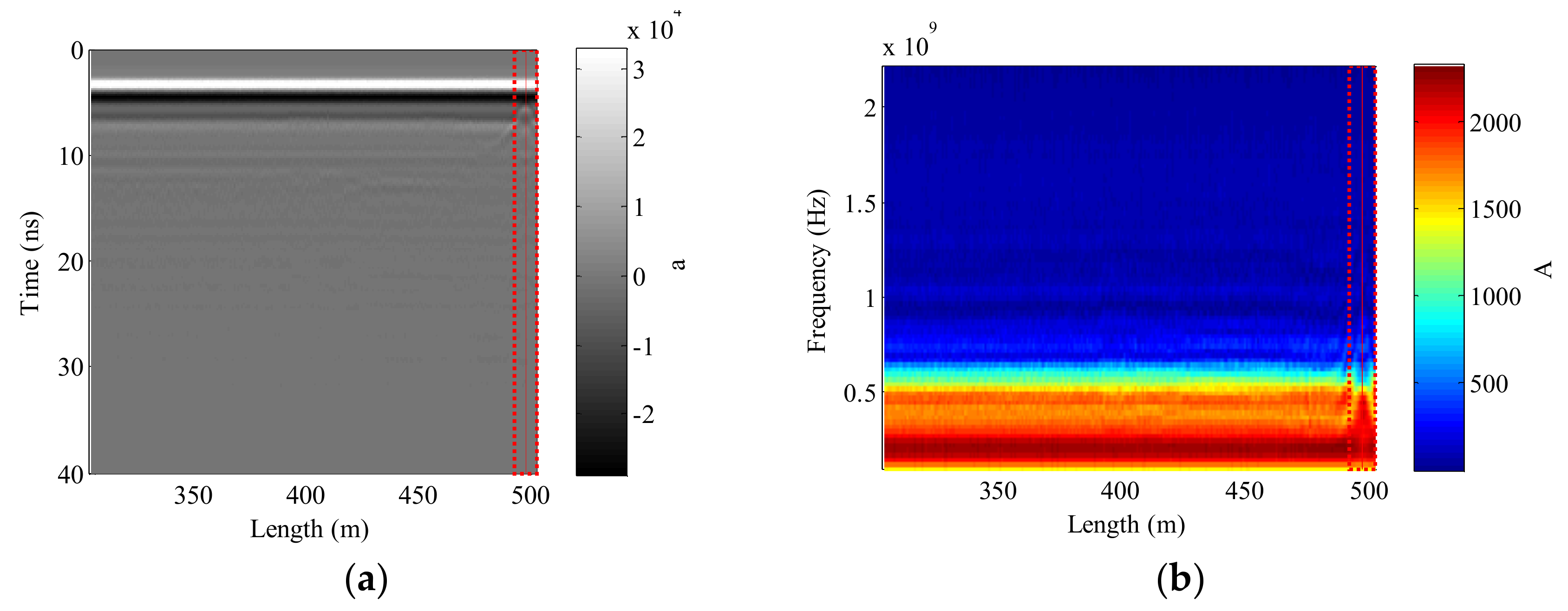
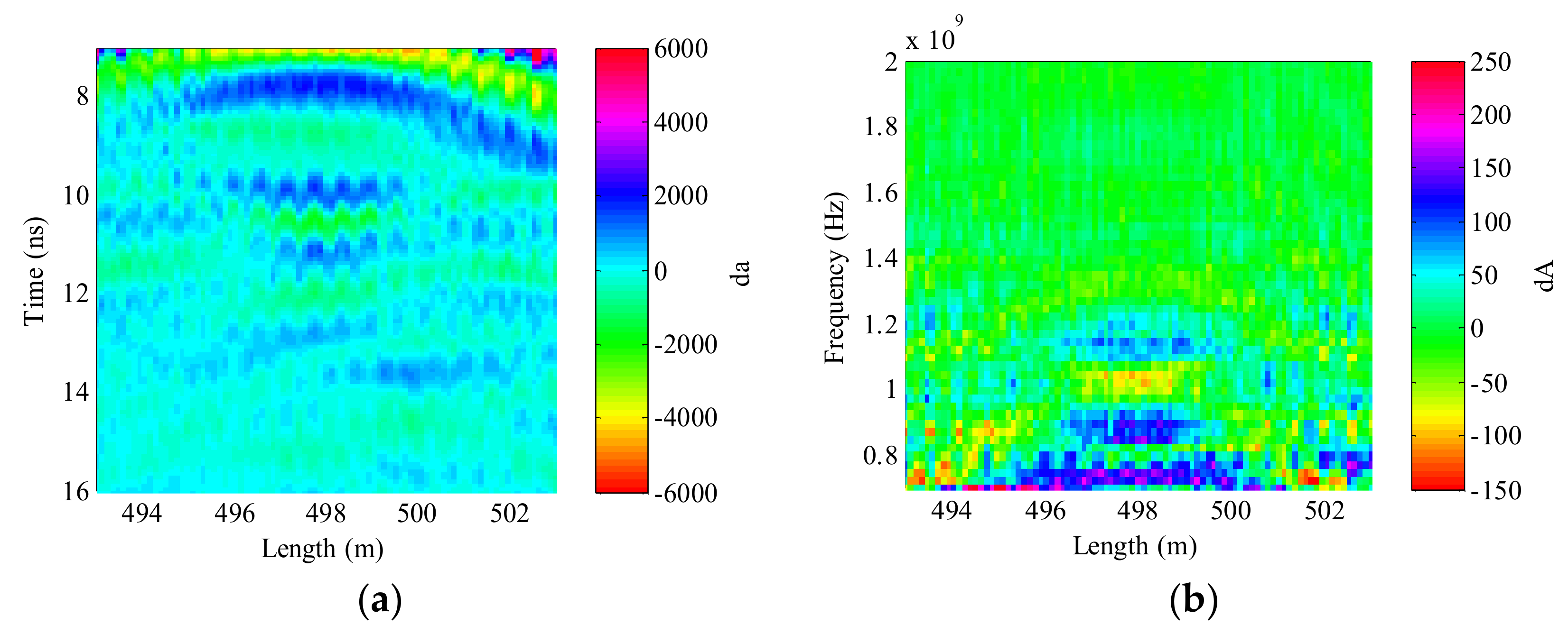
3.2.1. Range Selection of GPR Signal in Time and Frequency Domains

The first step was to establish a range, in the time and frequency domains, that corresponds to segments of each acquired trace of the GPR signals that are considered to better reflect the changes in the track condition at subsurface layers level [15,35,40,63].

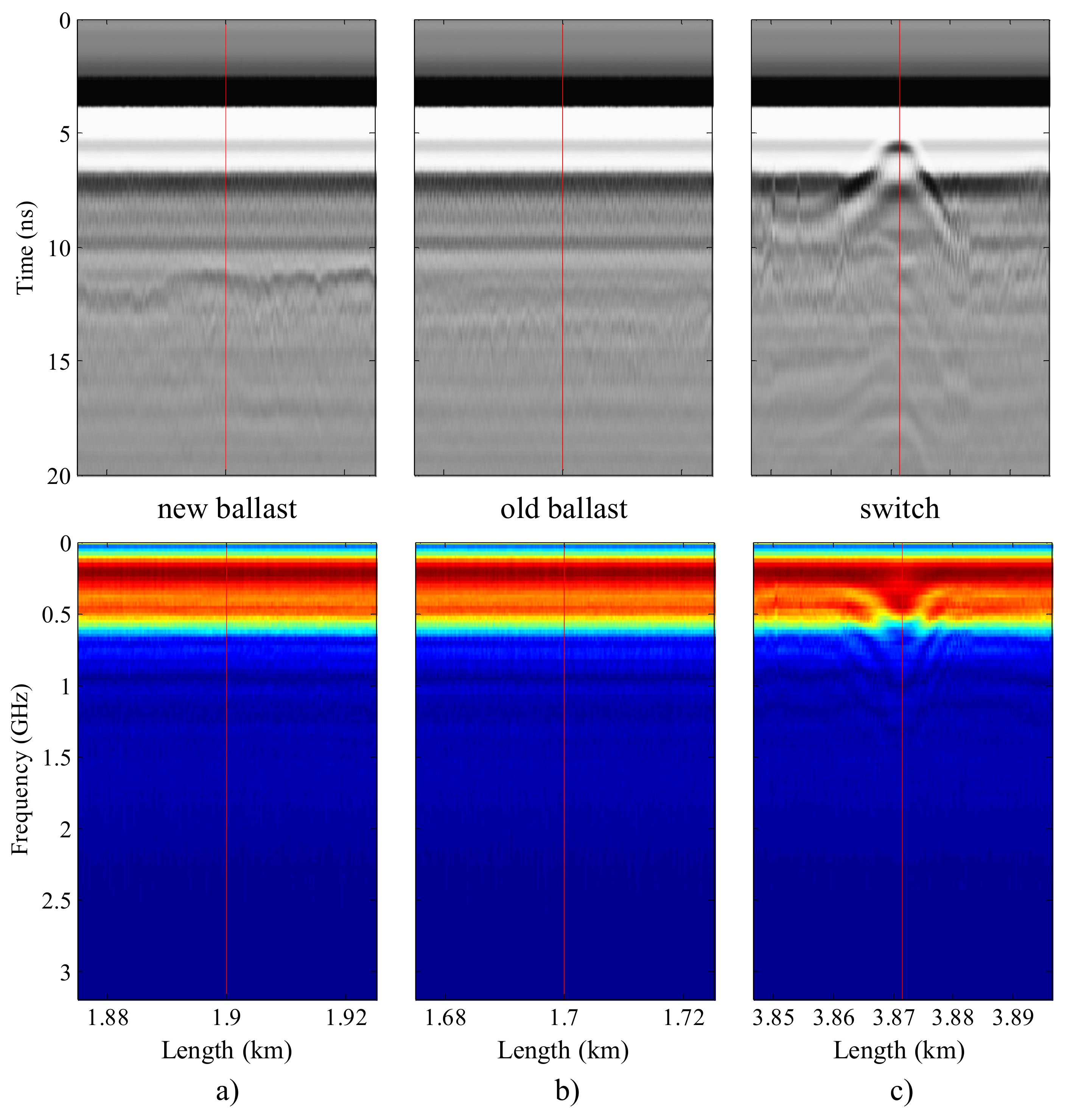
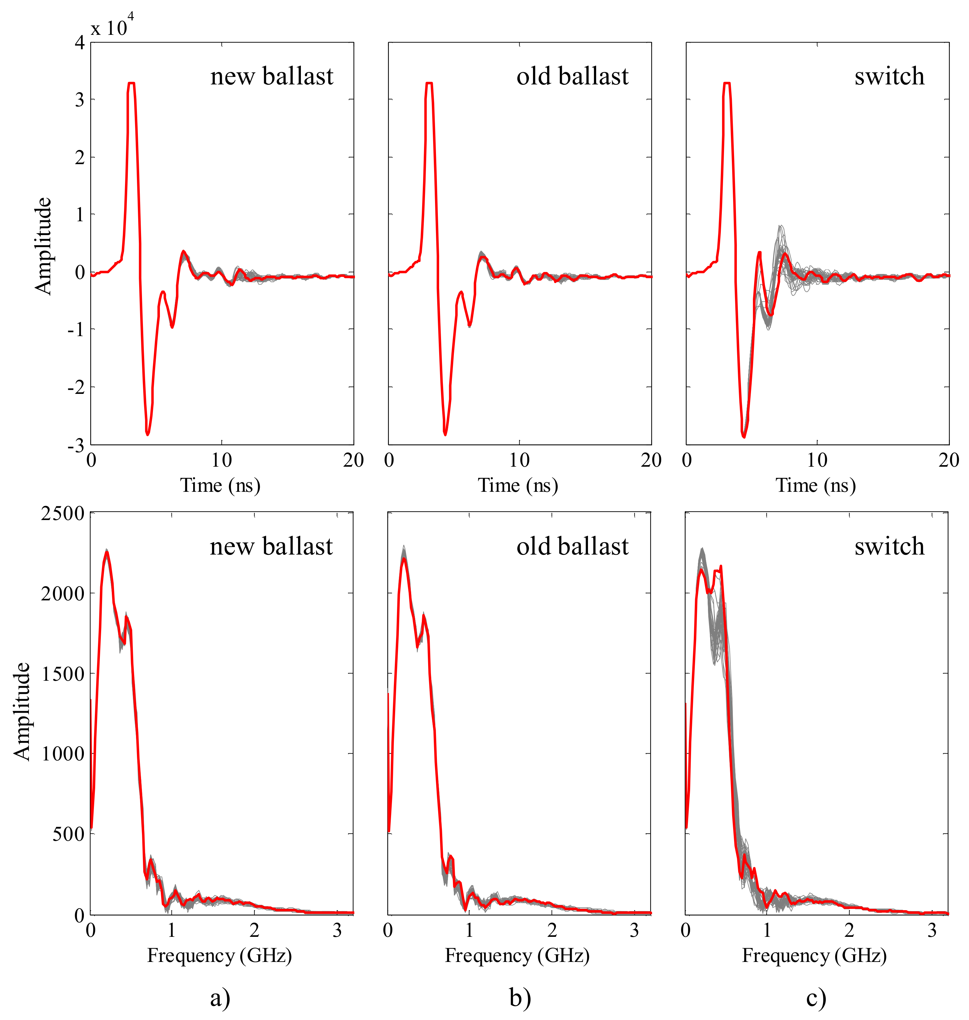
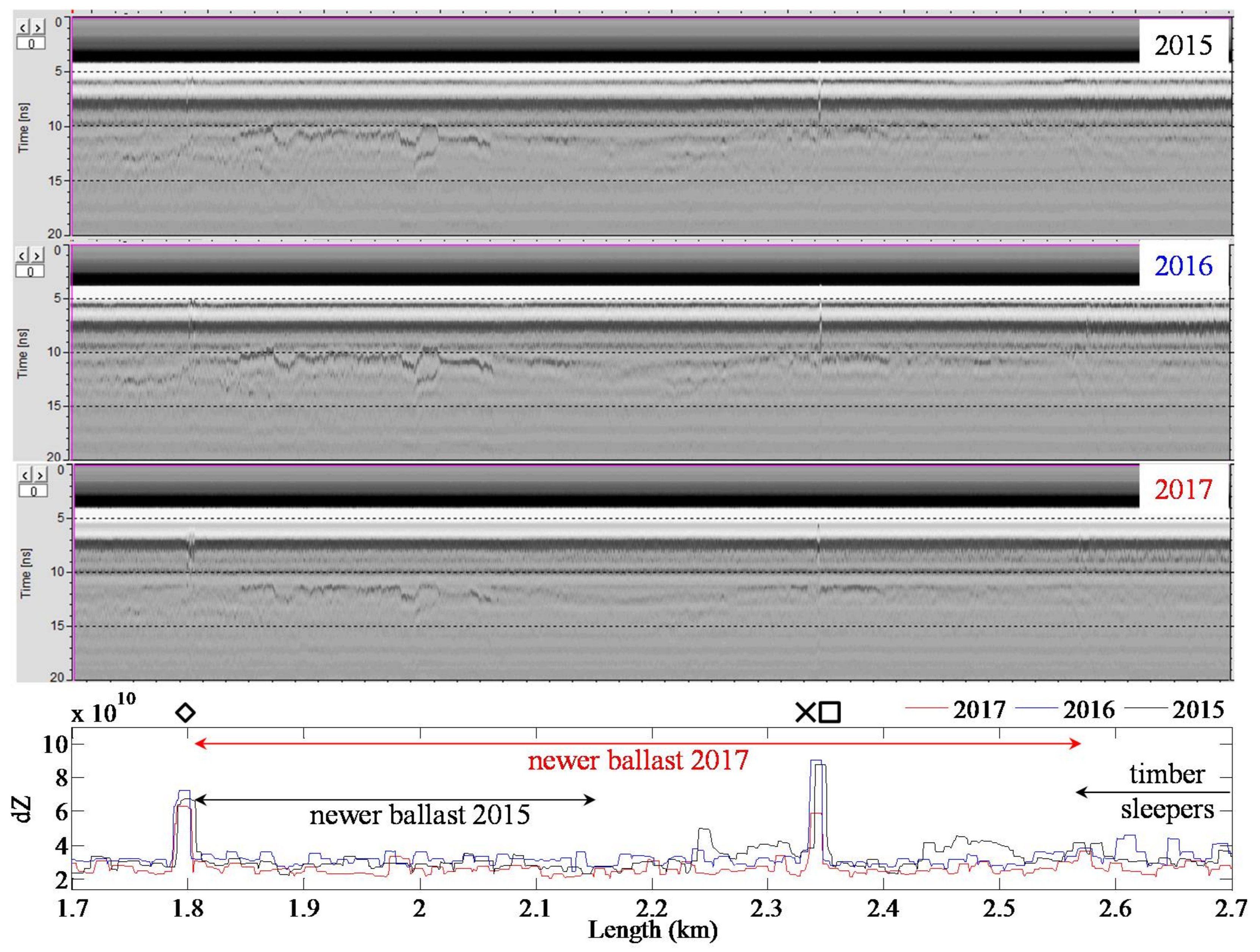
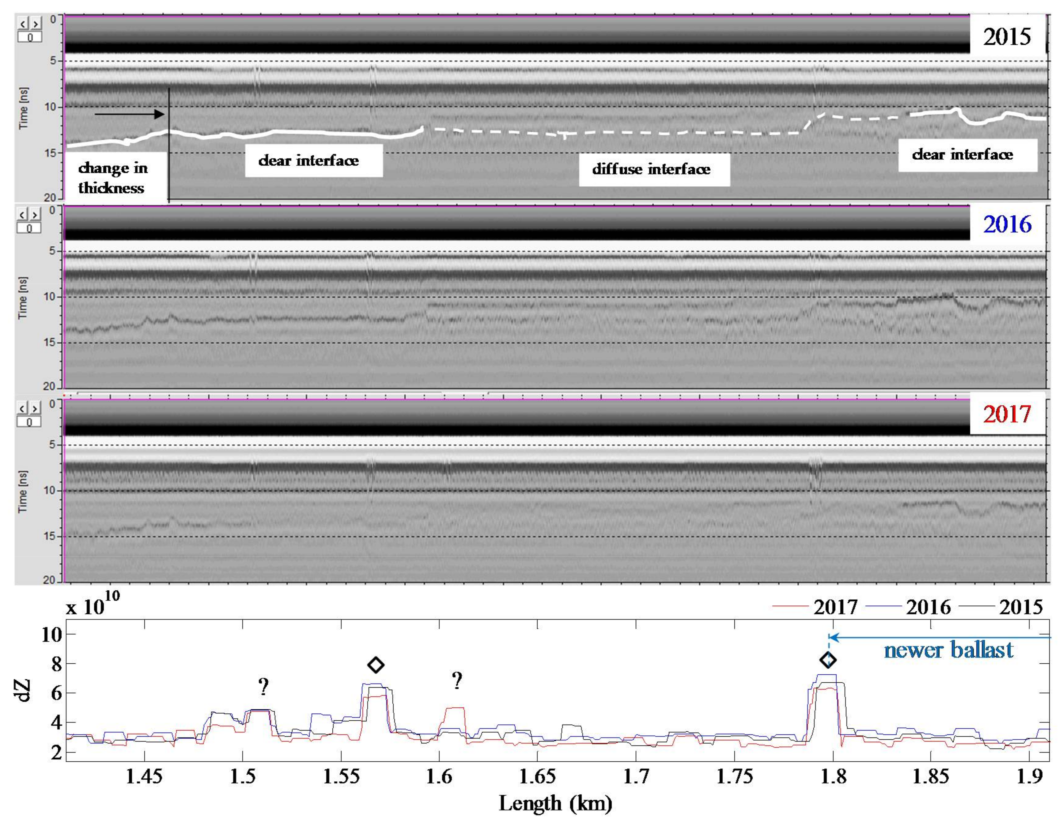
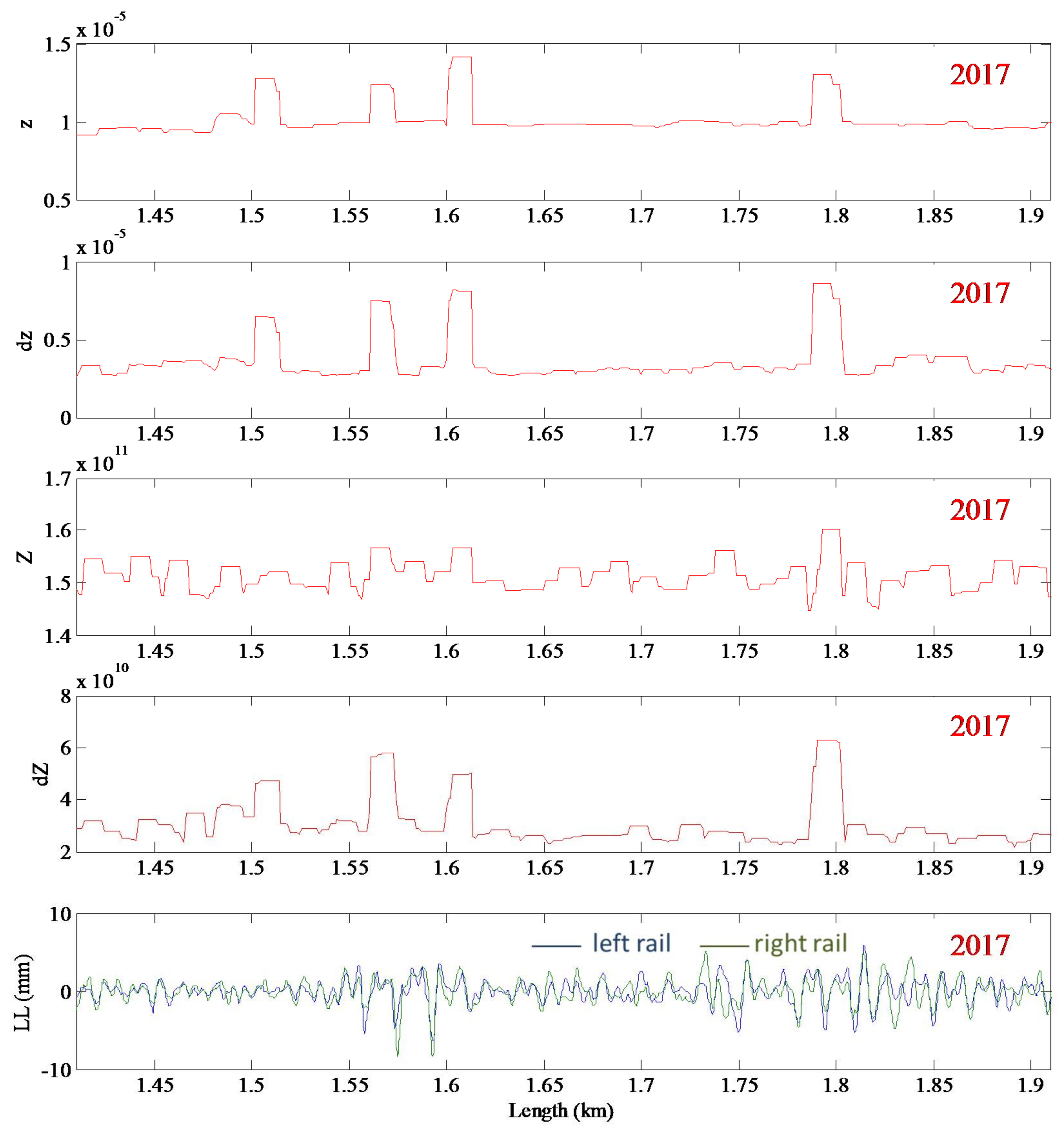
• In the time domain, several in situ GPR measurements performed on existing lines, with different characteristics (sleeper’s type and material, ballast fouling level, age of the track, with and without sub-ballast layer) were analysed [2]. Based on this analysis, a time window between 7 ns and 16 ns was selected for this study (see, for example Figure 1 and Figure 2), which was considered representative of the conditions of the ballast and subgrade.
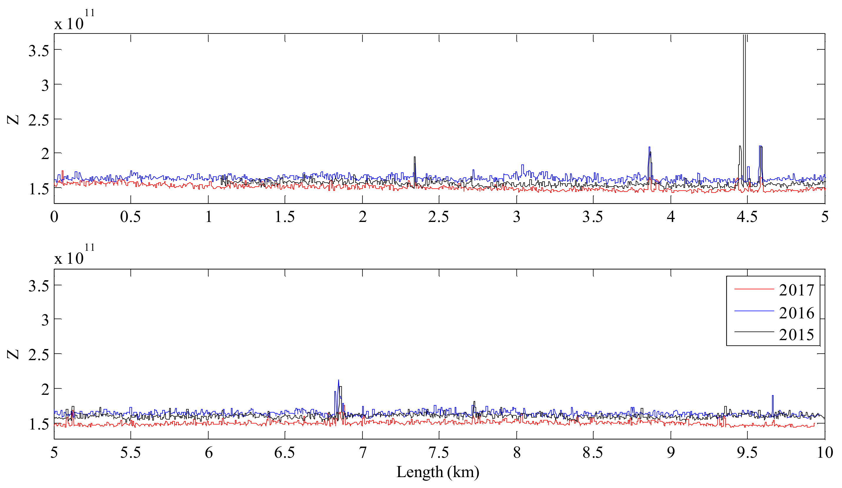
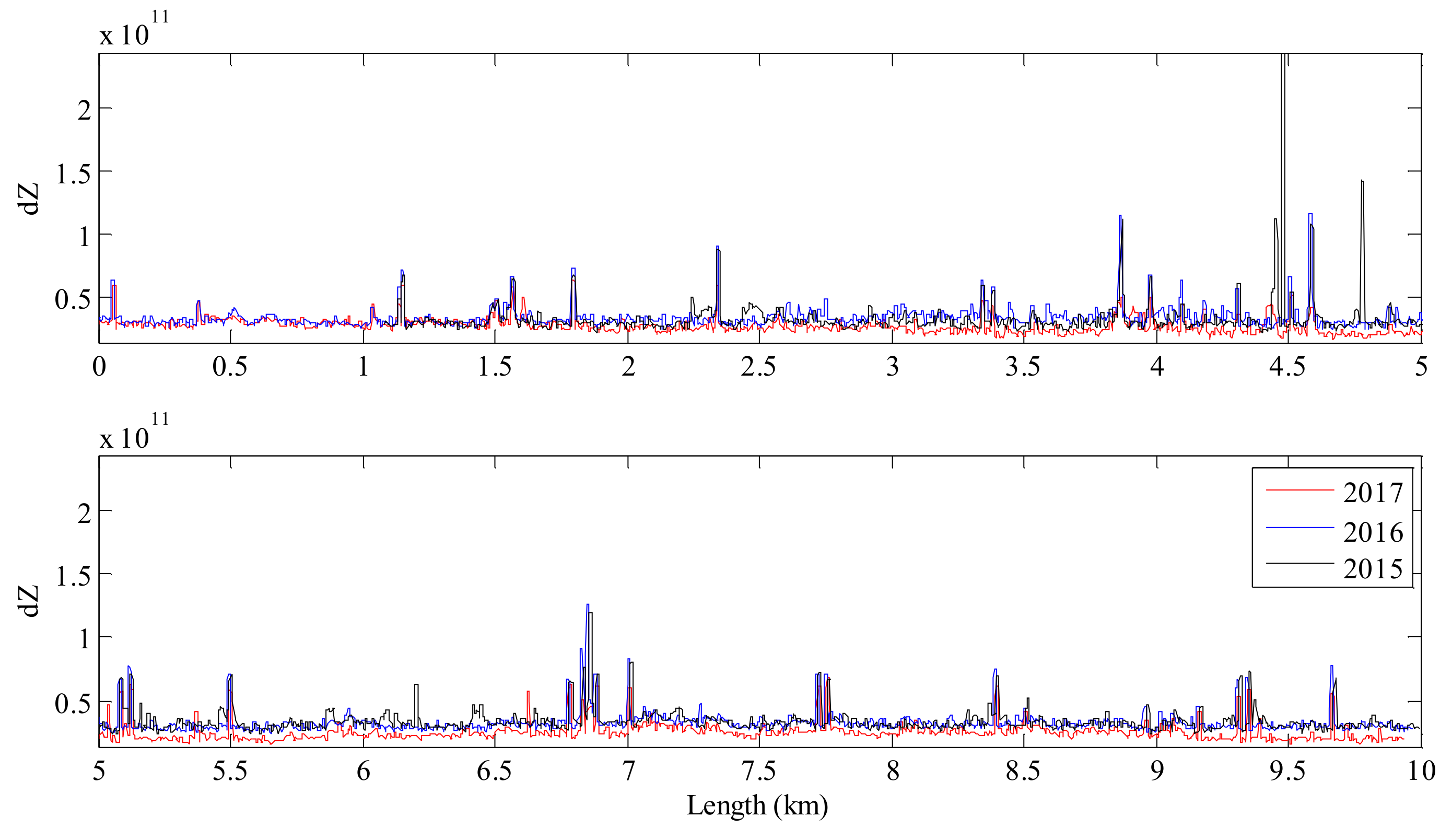
• In the frequency domain, numerous in situ GPR data were analysed in order to detect areas of the electromagnetic spectrum affected by changes occurring along the track. A range between 0.7 GHz and 2.0 GHz was selected (see for example Figure 1 and Figure 2). The changes induced by elements of the superstructure such as switches, sleepers and level crossings, are generally registered at lower frequencies (below 0.7 GHz), they were excluded because the main purpose was to detect ballast and substructure pathologies. The selection of the frequency range is in accordance with the information in the literature [15,63].

It should be noted that both time and frequency ranges should be adjusted to the type of antenna used, to its frequency and to its vertical position with respect to the track.

These threshold values depend on many factors, such as the type of rail, material of the sleepers, material and geometry of the ballast layer, material and geometry of the track platform. Therefore, for the implementation of this method at the network level, a set of threshold values need to be established, which will depend of the characteristics of the track, followed by a preliminary validation with field surveys with some pit holes.

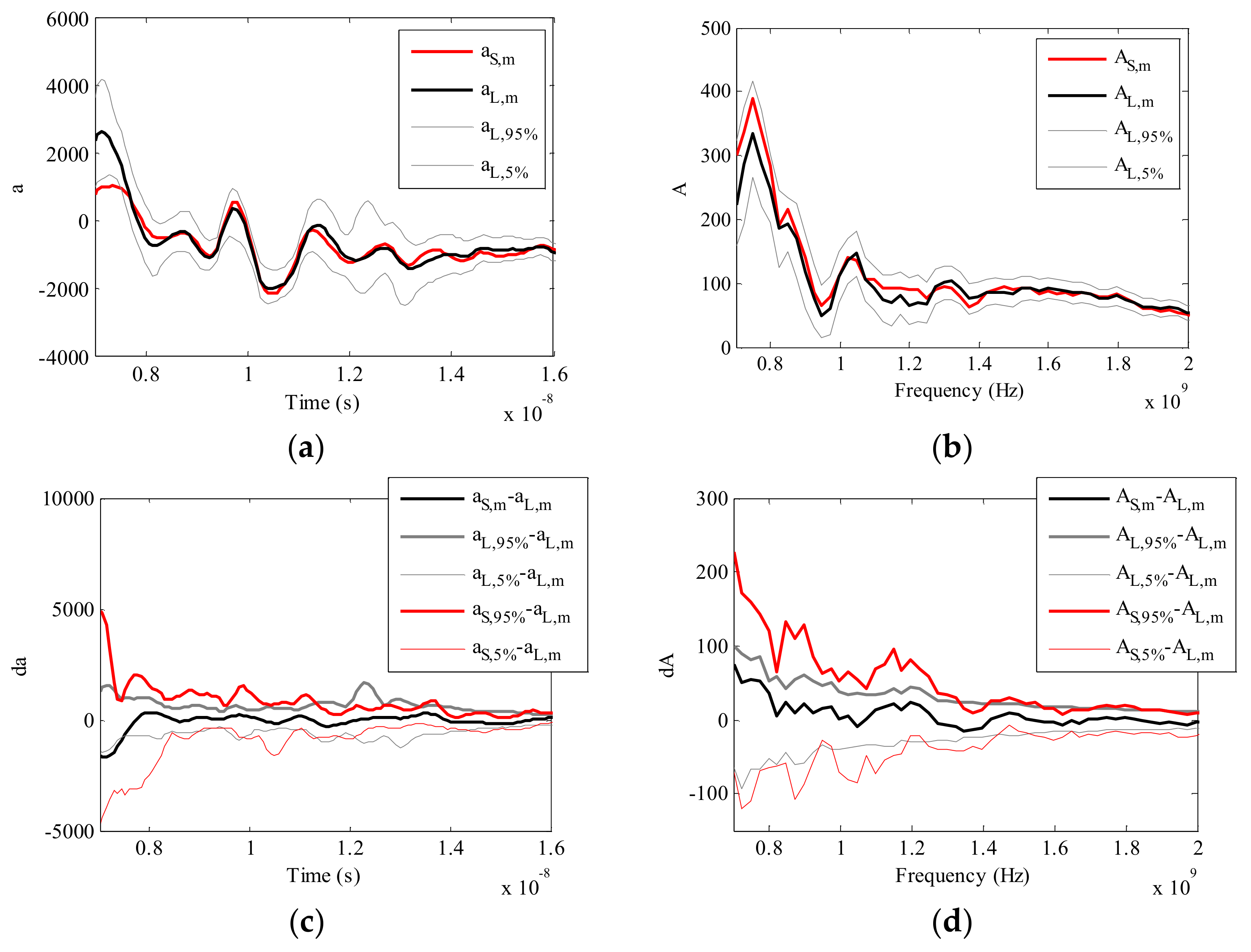
3.2.2. Sliding Window for Track Changes Detection

The second step consisted in comparing some characteristics of the GPR signals in a short ($S$) sliding window with those in a long ($L$) sliding window.

The lengths of the sliding windows adopted in this study are $S$ = 10 m and $L$ = 200 m, for the short and long windows, respectively. These parameters were identified as follow:

• Several dimensions for the long and short windows were tested and also the positioning of the small window within the large one was varied;
• The length of the shorter window (10 m) was selected to be representative of the length of the track defects that typically occur at ballast and subgrade levels [2,64,65];
• The length of the longer window (200 m) was selected in order to reflect the length of the track adopted by railway engineers, when analysing track geometric parameters, for track quality classification and for tamping planning [66,67].

The length of the sliding windows can be adjusted depending on the purpose of the study, namely on the length of the defects or anomalies to be detected.

The differences between the signals acquired in the two sliding windows allow identifying changes in track characteristics, both in the time and in the frequency domain (see Section 3.2.3).

The comparison that it is made between the two windows does not filter out any GPR signal. It is meant to only to detect differences in its amplitude along the track. Therefore, it differs from other approaches, such as the horizontal background removal that is used in other applications, but is clearly unwanted for the assessment of layer interfaces in transport infrastructures, as it can delete continuous horizontal information that corresponds to infrastructure layers.

3.2.3. GPR Expedite Parameters Definition

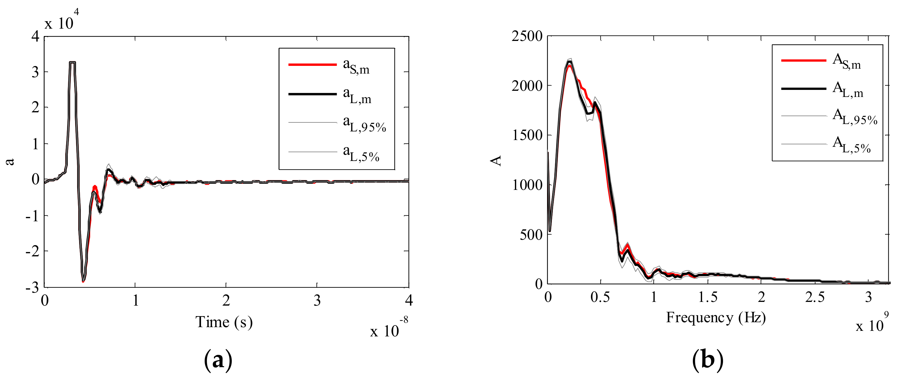
The third step of the proposed approach consists in calculating four new parameters. These parameters aim to analyse GPR data, obtained in railway tracks, in a more user-friendly way for “non-GPR professionals” and to identify locations in the track where changes in the infrastructure occur. The parameters used in this approach are:

• in time domain, $z$ and $dz$;
• in frequency domain, $Z$ and $dZ$;

which are defined by the following equations:

$$z={{\displaystyle \int }}_{t_1}^{t_2}\left|a\right|dt$$

(1)

$$dz={{\displaystyle \int }}_{t_1}^{t_2}\left|a_S-a_{L,m}\right|dt$$

(2)

$$Z={{\displaystyle \int }}_{f_1}^{f_2}\left|A\right|df$$

(3)

$$dZ={{\displaystyle \int }}_{f_1}^{f_2}\left|A_S-A_{L,m}\right|df$$

(4)

where: $a$ and $A$ are the GPR signal amplitudes in the time and frequency domains, respectively; subscripts $S$ and $L$ denote the short and long sliding windows and $m$ denotes the averaged signal in the specified window; $t_1$ and $t_2$ are the lower (7 ns) and upper (16 ns) values of the time interval of the signal under analysis; $f_1$ and $f_2$ are the lower (0.7 GHz) and upper (2.0 GHz) values of the frequency range of the signal under analysis. Therefore, $z$ and $Z$ correspond to the areas under $\left|a\right|$ and $\left|A\right|$ plots, respectively in the selected time and frequency ranges, while $dz$ and $dZ$ correspond to the differences in area of the GPR signal amplitude between the short and long sliding windows, also respectively in the selected time and frequency ranges.

3.3. Example of Signal Processing for Methodology Implementation

Figure 3 presents examples of the original signal amplitude in the time (a) and frequency (b) domains, in terms of the mean or averaged signal (denoted by subscript $m$) over the shorter ($a_{S,m}$ and $A_{S,m}$) or longer ($a_{L,m}$ and $A_{L,m}$) sliding windows; percentiles 5% and 95% of the longer window are also plotted to illustrate the variability of the signal.

The examples presented in Figure 4 depict the different steps of GPR signal processing in a normal section of the track: (i) the time (a) and frequency (b) ranges selected for the analysis in order to better reflect the changes in the track condition and (ii) the differences in the amplitudes of the signal ($da$ and $dA$) in the time (c) and frequency (d) domains, when comparing the results between the short sliding window and the large sliding window.

Examples of spectrograms of a and A, over a length of 200 m (the larger sliding window—L), are presented in Figure 5 with the identification of the short sliding window inside the dotted red rectangles.

Examples of spectrograms, calculated as the difference between the amplitudes of the short window ($a_S$ or $A_S$) and the mean signal of the large window ($a_{L,m}$ or $A_{L,m}$) from Figure 5, are presented in Figure 6, in the time (a) and in the frequency (b) domains.

4. Application of the New Method to a Case Study and Discussion of Results

Examples of the proposed methodology application to a track section of an existing line are presented in this section. For confidentiality reasons the GPS location is not revealed and the location reference is not the real one. The GPR data used to illustrate the application of the approach were acquired with the 400 MHz antenna referred in Section 3.1.

Figure 7, Figure 8, Figure 9 and Figure 10 depict examples of $z$, $dz$,$Z$ and $dZ$ values, considering sliding window lengths of $L$ = 200 m and $S$ = 10 m, calculated for a 10 km stretch of an in-service railway line, obtained from GPR signals acquired in the summers of 2015, 2016 and 2017 (in black, blue and red, respectively) and considering $t_1=$7 ns, $t_2=$16 ns, $f_1=0$.7 GHz and $f_2=$2.0 GHz, as mentioned above.

It is observed that the variable $dZ$ yields somewhat flat plots interrupted by prominent peaks, which correspond to changes in the GPR signal in the selected frequency range. The authors suggest that this variable might be more appropriate for the proposed approach, though further studies should be performed to test the applicability of this method to other scenarios or other parameters.

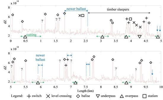
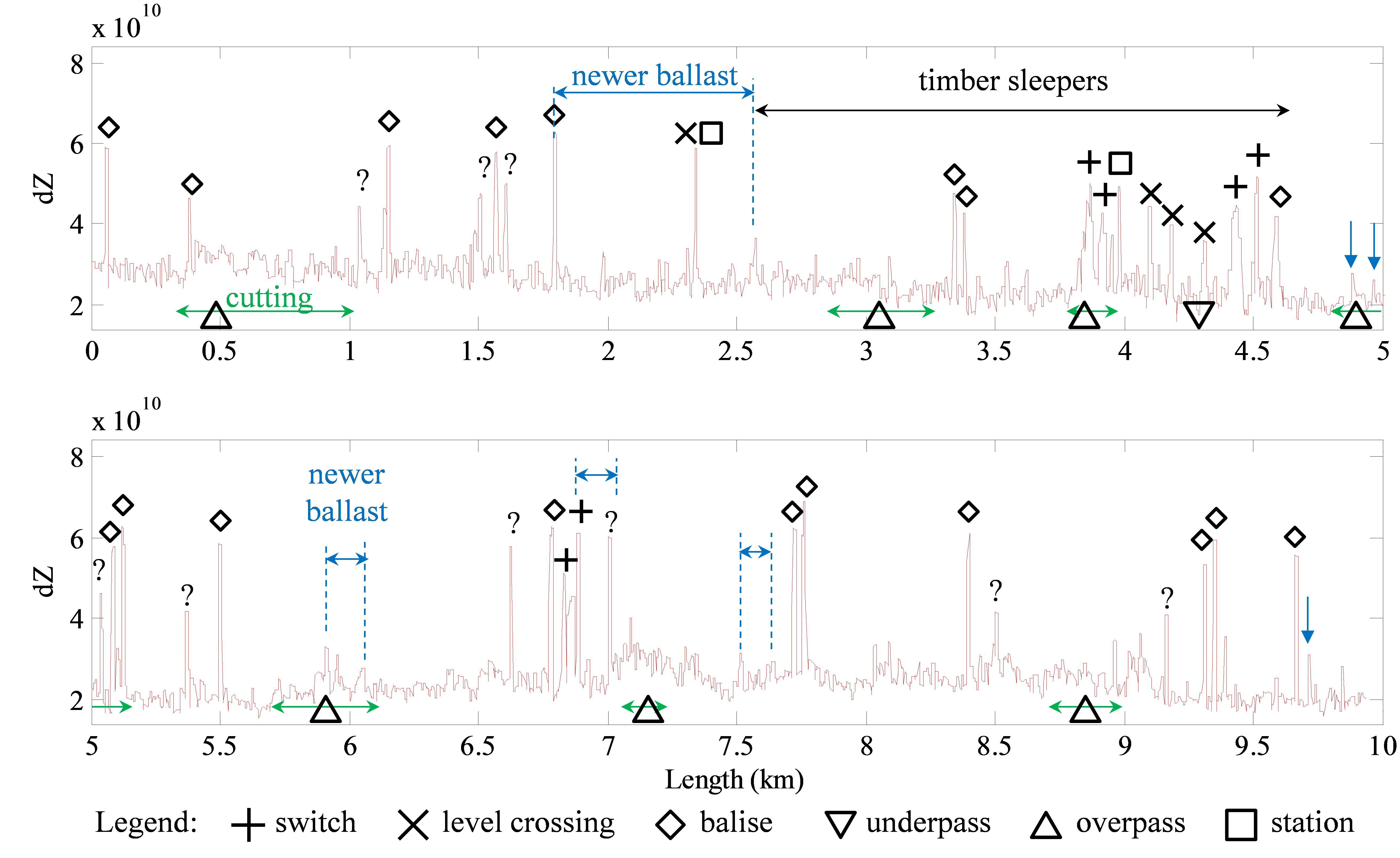
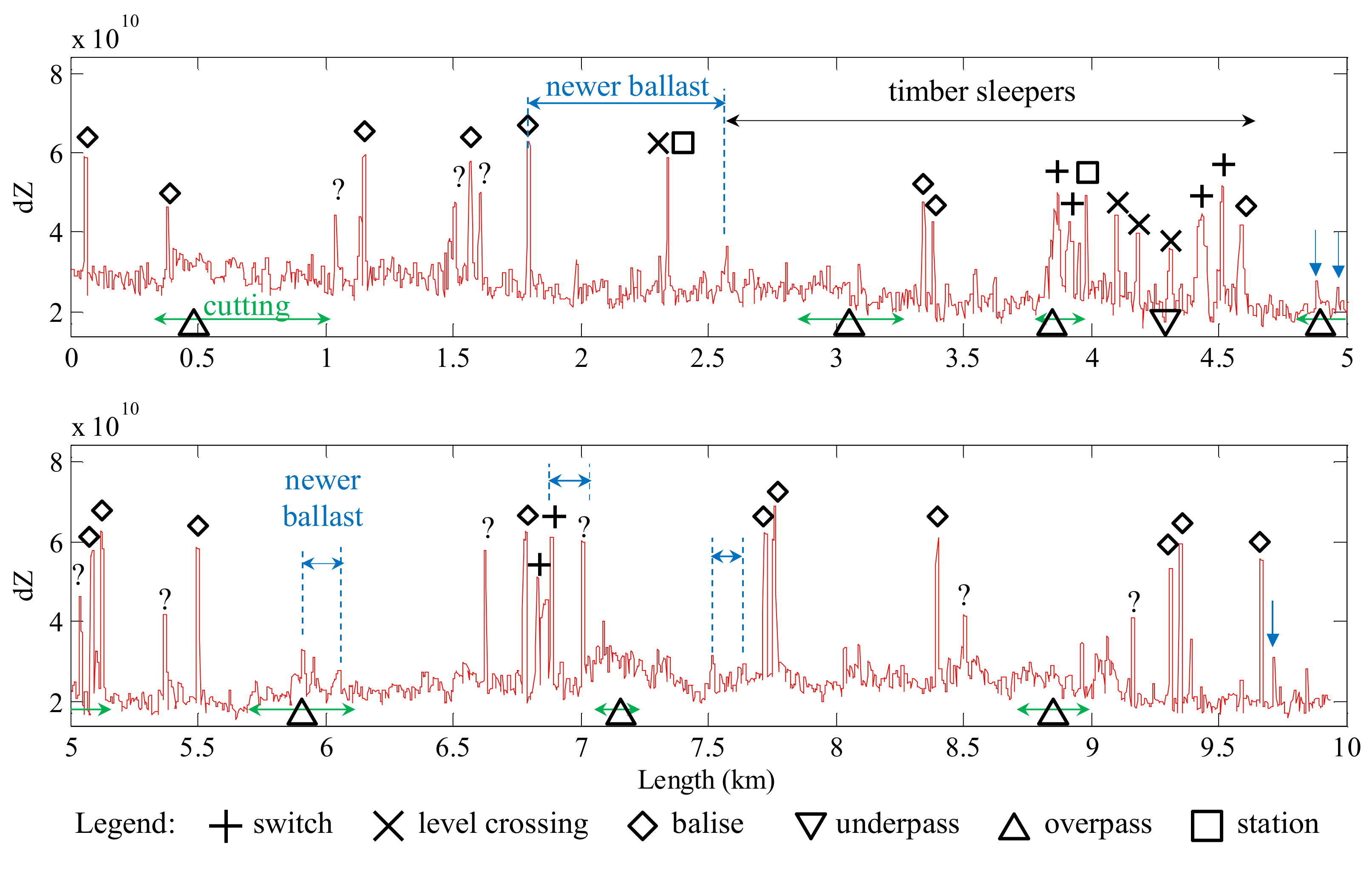
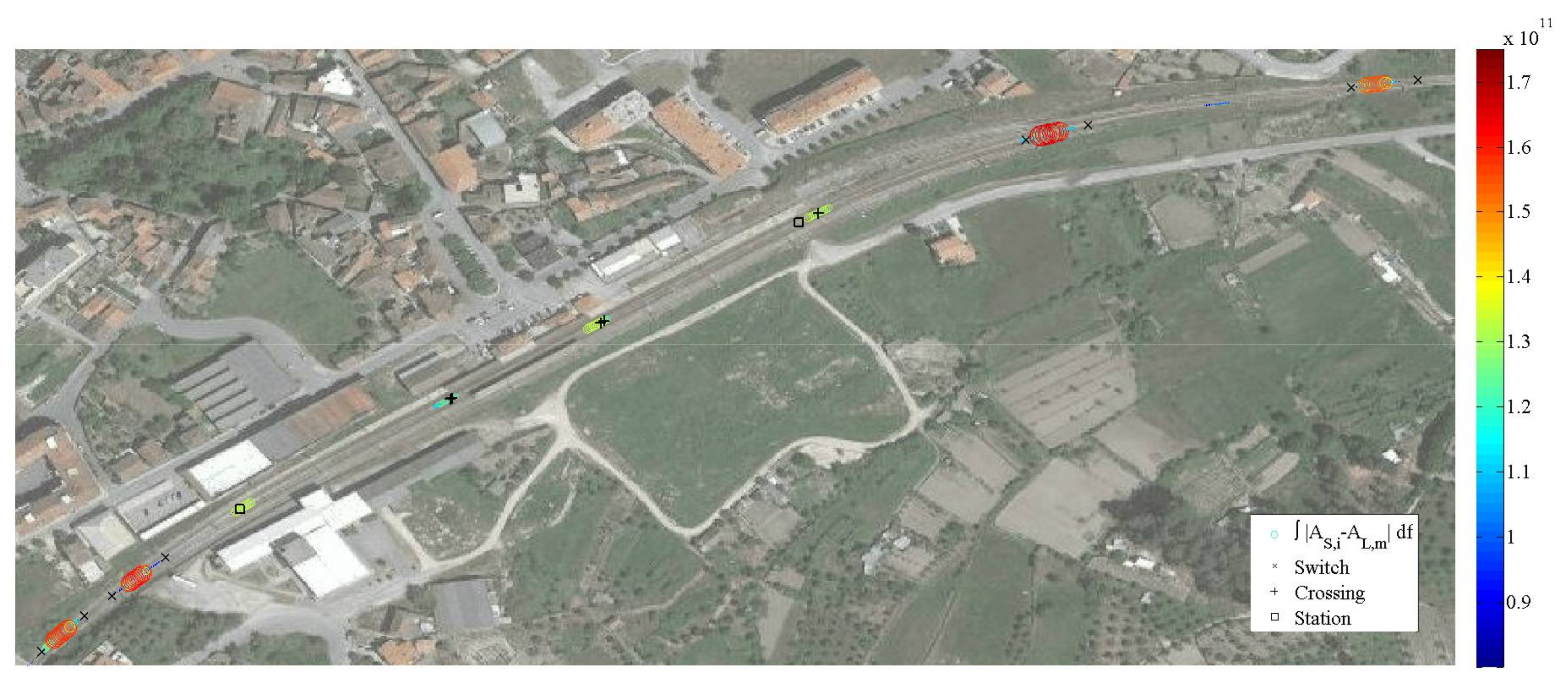
4.1. Event Identification

This first application of the methodology it is recommended to be undertaken always in the beginning of the overall analysis of a track, in order to identify track events and to enable a location validation of the GPR results. Consequently, it will provide a good correlation of GPR results with track geometric parameters.

It was verified that the most noticeable peaks in these variables corresponded to the locations of switches and crossings of that line, which significantly disturbed the GPR signal, and were quite clear in all surveys, year after year. Figure 11 presents the identification of the events, cutting zones and sections with new ballast in the $dZ$ parameter of GPR 2017 measurement.

In Figure 11, the squares denote the beginning and end of the station platform, the saltires (diagonal crosses) denote the switches, the crosses denote the level crossings, the downward pointing triangles denote underpasses, the upward pointing triangles denote overpasses and the diamonds denote the balises (from the CONVEL system used for the automatic train protection). Many other peaks were identified but were found to be unrelated to any known singularity in the track, which were identified using question marks in Figure 11. It is possible that such remaining peaks could be related to unwanted discontinuities in the track structure or locations where the structure has been altered, with respect to the surrounding sections of the track. Such differences could be related to different track components or to track pathologies such as poor drainage or ballast fouling.

Figure 12 shows different aerial photographs highlighting examples of the identified singularities.

Figure 13 shows the locations on the track that correspond to the highest peak values identified in the previous plots, considering a stretch of that line with multiple singularities, passing through a train station. It is visible that these singularities are clearly identified using the $dZ$ parameter.

Therefore, it is recommended to use the $dZ$ parameter as pre-analysis of each campaign, in order to correlate the events location and guarantee that the data analysed are in the same locations in different campaigns.

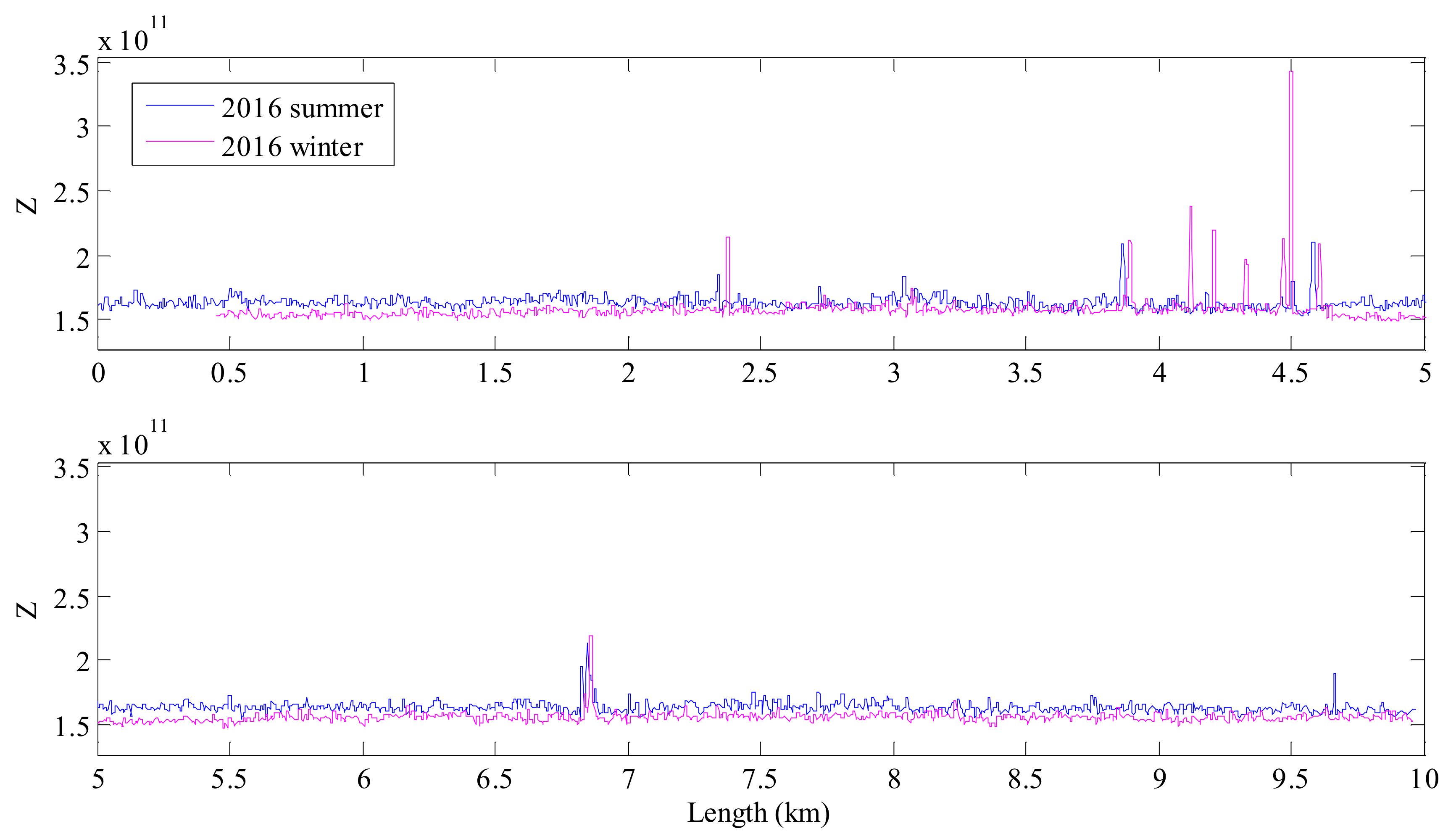
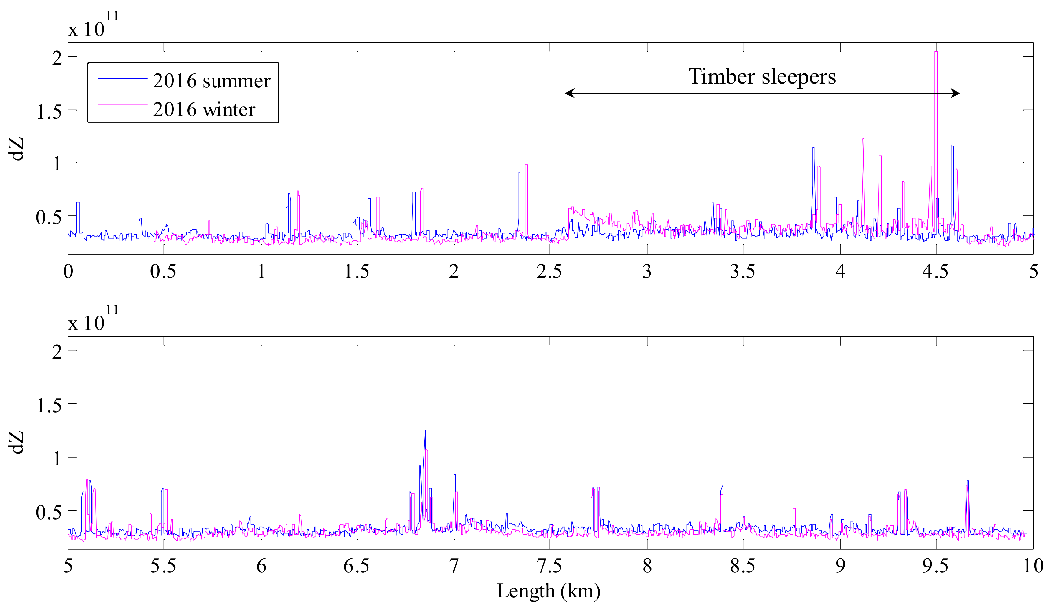
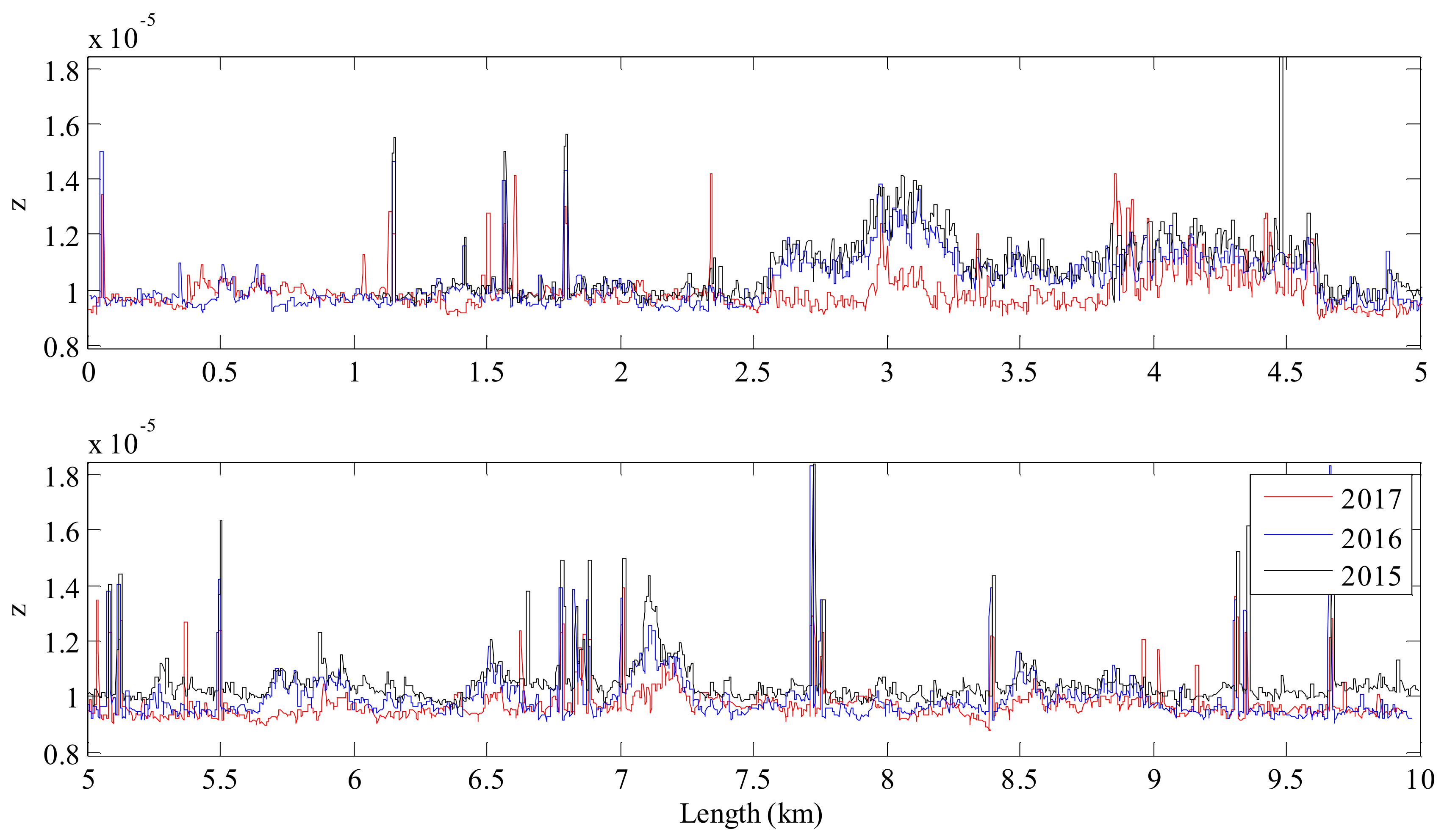
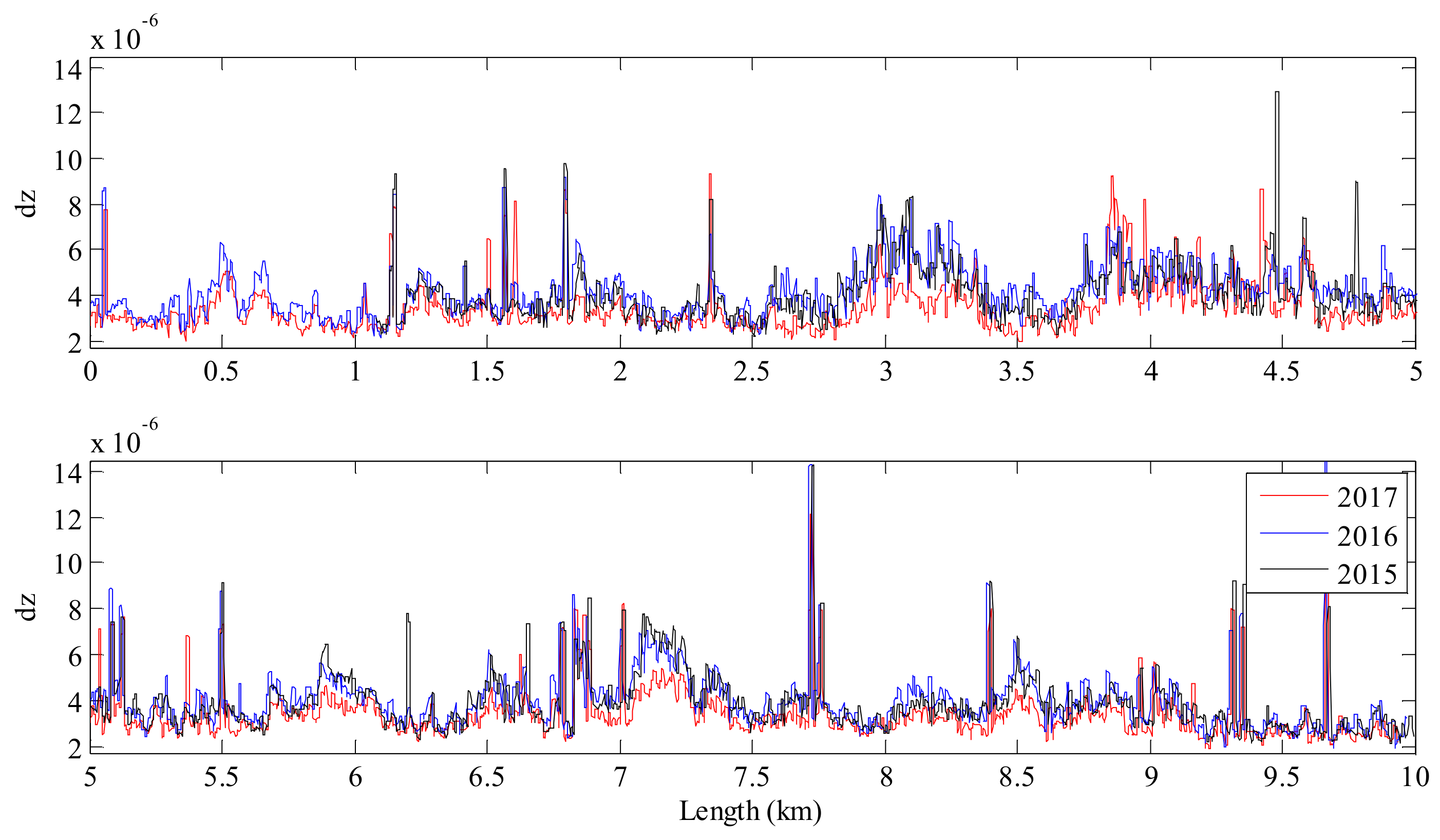
4.2. Sistematic Comparison between Consecutive Campaigns

This second application of the methodology is efficient for track management decisions, as enable the following of the track condition evolution in time. Also, it can be used, when several campaigns are available to forecast the track behaviour.

This can represent an important tool for identification of sections that are deteriorating at a faster rate along the track. To implement the methodology for this purpose it is essentially to have all the information on the maintenance and rehabilitation actions that were undertaken between GPR testing campaigns for cross checking.

To illustrate the potential of the proposed approach to identify changes in the track structure/condition, the authors analysed in more detail the locations with peaks in the variable $dZ$ that were not directly associated with locations of known track events. For this purpose, three different sets of GPR data obtained in the summers of 2015–2017 on the same stretch of line were compared. Firstly, the main purpose was to study the locations identified by the questions marks in Figure 11, and assess their coherence when comparing the three surveys. It was noted that some of those locations (those not related to any track event) were not present in all the surveys.

As an example, two track sections are presented herein. The first one is a section where the ballast was renewed between the 2015 and 2016 GPR surveys. The second one is a section where the $dZ$ values were systematically higher than in the surrounding sections of the line in the three analysed surveys.

The first example corresponds to a location where ballast was renewed in 2 phases: one before the 2015 survey (from 1.80 km to 2.15 km) and the second one after the 2015 survey (from 2.15 km to 2.58 km). Figure 14 shows the sections with renewed ballast in 2015 and in 2017. The graph of $dZ$ obtained in 2015 has generally higher values (black line) in the section that was only rehabilitated later on; on the other hand, the graphs obtained in 2016 and 2017 have similar values, lower than in 2015.

The results show the potential of the proposed approach to detect distinct areas, when comparing inspection surveys performed in consecutive years. The proposed analysis in the frequency domain allowed observing dissimilar results even if the difference between the GPR raw signals was not clear in the radargrams of the 2015 survey, or in the latter surveys. This dissimilar behaviour can constitute a trigger in future automated GPR data analysis that identifies the need for further processing of the GPR in this section. So, it can be observed that the analysis of the differences in the frequency domain enabled to identify the response of the GPR signal in a section where track rehabilitation was performed.

The second example is a section located between 1.47 km and 1.60 km, which yielded higher $dZ$ values in all the surveys, even in locations that were not associated with any track event. Figure 15 presents the radargrams obtained in this section during the three GPR surveys and the corresponding $dZ$ plots. From the radargrams it can be observed that this section is quite heterogeneous both in terms of ballast thickness as in the “clearness” of the interface between ballast and subgrade layer. The increase in the $dZ$ values may be caused by the change in thickness that occurs at approximately 1.47 km. Again, this result illustrates the potential of the analysis in frequency domain to identify sections that are dissimilar, and therefore require an in-depth interpretation of the GPR data.

Figure 16 presents an example of a possible visualisation of the GPR signal information together with track geometric parameters, namely the Longitudinal Level (LL). The section presented is the same as the one illustrated in Figure 15. It can be observed that there is an increase in the LL values in the same location where the values of $dZ$ increase, between 1.47 km and 1.60 km. The systematic correlation between those parameters requires further research and validation with extended field data.

It was demonstrated that the proposed approach can perform an efficient identification of dissimilar sections along the track, which can be considered as requiring a deeper analysis.

After identifying sections with distinct behaviour, more detailed interpretation can be performed and additional NDT can complete the diagnosis of the track condition in these sections. Additionally, information on traffic change along the line is important for a thorough analysis of the track increased rate deterioration.

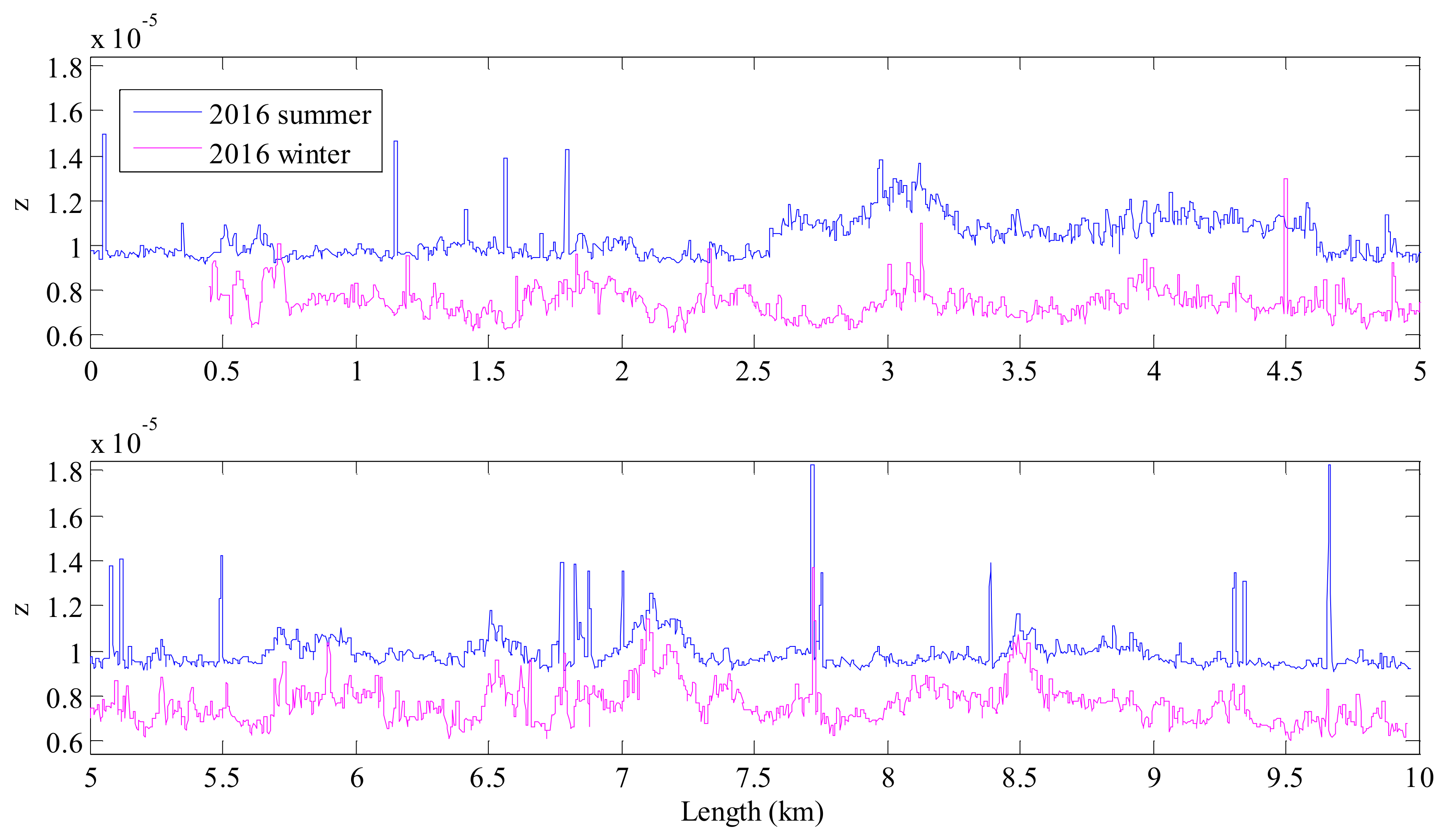
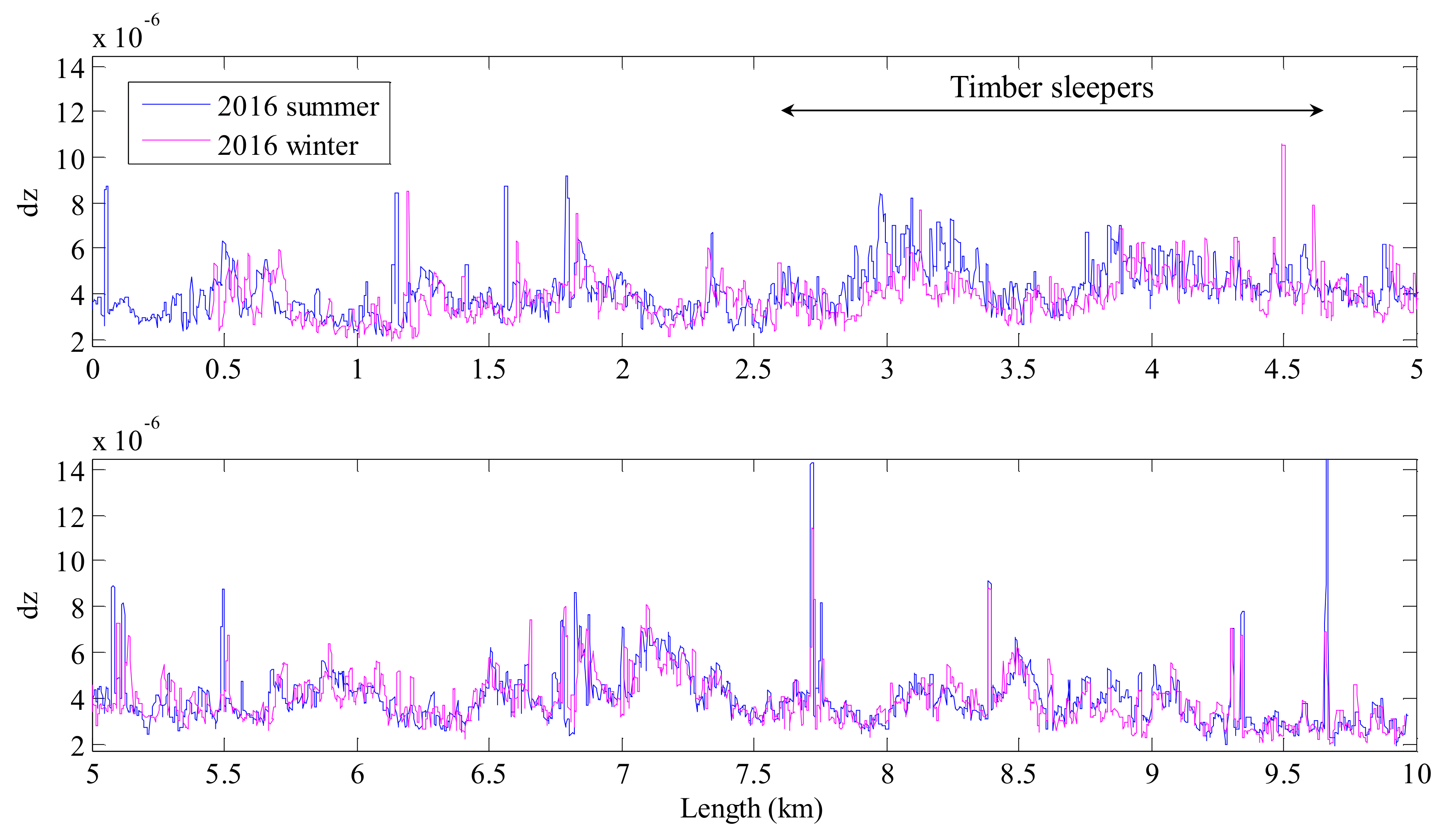
4.3. Analysis of Seasonal Influence on the GPR Data

The comparing of the GPR campaigns performed in different seasons, with different water contents of the ballast and substructure, represent a tool for identifying sections with ballast fouling and drainage problems. As already referred to in Section 2.1, the fouling of the ballast promotes the water trapping in this layer and, consequently, has a negative impact on track behaviour. This phenomenon is more evident when compare the same section in different hydraulic conditions, namely in dry and wet season. On one hand, if the track structure is healthy and the drainage is proper, no difference is detected between campaigns performed with GPR antennas with the frequency used in this study. On the other hand, if there are drainage problems of ballast fouling, the water content in the track layers will lead to attenuation of GPR signal.

To illustrate this application, two GPR surveys performed in the same year, but in different seasons were analysed. The GPR measurements were undertaken in January, after a few days of rain, and in July, in a dry and warm period. When comparing the values of parameter $z$ (in time domain), it is clear the different behaviour of the GPR signal between winter and summer (see Figure 17). The significantly reduced values in winter may be explained by the attenuation of the signal with higher water content in the assessed media [2]. On the other hand, when comparing the same parameter $z$ for the different surveys performed all during summer, the values are similar (see Figure 7).

The difference represented in the graph (see Figure 17) reflects the GPR signal shape in time domain. The GPR signal is most commonly processed in time domain [2,11,26,38,45] by: (i) calculating the layer thickness using an “default” dielectric value, generally assumed valid for the type of material tested; or (ii) by performing test pits at some locations, measuring the real thickness of the ballast and, based on this, calculating the real dielectric value and adopting this value for processing all the signal along the track. In case of homogeneous media, such as concrete or asphalt, these assumptions are close to the real situation. However, in case of non-homogeneous media such as ballasted railway track, and particularly in old existing lines, there are several factors that affect significantly the dielectric properties of the media along the track. Among those, the two main factors are the level of ballast fouling and the water content. Both affect the GPR signal by reducing the wave speed propagation and attenuating the signal intensity. Nevertheless, they are difficult to dissociate from each other, as their effect is combined [2,25,38], unless in situ samples of material are collected and analysed in laboratory in order to characterise the grading, fouling level and water content. Nevertheless, this only characterises specific locations, as old tracks are quite heterogeneous in terms of materials and drainage conditions. Thus, assuming a constant or “default” dielectric value for the ballast material throughout the line or when comparing between summer and winter GPR surveys, may induce wrong estimates of the thickness of the layers. Therefore, when comparing the two surveys in Figure 17, the differences between them do not correspond to real differences on the track, rather reflecting the influence of the testing conditions, mainly as the different water content of the ballast and the subgrade. In case of GPR processing in time domain, when comparing two campaigns, the information given by z parameter enable the choose of different “default” dielectric constants, to better reflect the influence of the water and turn the processing more realistic.

Instead of representing the results of the two surveys in the time domain in terms of $z$, the data can be represented in terms of $dz$: see Figure 18. In this case, the results become quite similar between the two surveys. It is noted that higher values are observed in the in the section of the track with timber sleepers.

Regarding the analysis in the frequency domain, it enables filtering most of the differences observed between the summer and winter surveys regarding parameters $z$ and $dz$ in the time domain. This is evidenced in Figure 19 and in Figure 20, with plots of $Z$ and $dZ$ values, respectively. Therefore, the authors suggest analysing the GPR results in the frequency domain, in terms of $dZ$, because it seems less influenced by the water content and, consequently, allows to associate changes in that variable with distinct zones of the track and, eventually, with possible track pathologies. For example, in Figure 17, it is clear the greater variability of $dZ$ values in the zone that corresponds to the track section with timber sleepers.

When sections with distinct behaviour are detected by comparing two campaigns performed in different seasons, these can be analysed further on; advanced signal processing techniques have to be used, taking into account scattering and dispersion phenomena as well as the level of ballast fouling, validated with material collected in situ and analysed in laboratory.

4.4. Final Remarks

GPR systems are already installed on inspection vehicles of many railway networks. However, the current and common strategy is to acquire and store the huge amount of data in datacentres, which are accessed punctually in the event of any pathology of the track structure or to estimate the percentage ballast fouling.

Possible future strategies to manage and process the huge amount of data acquired with GPR inspections should include automatic data processing to detect the early development of track pathologies, by using approaches similar to the one presented in this work. In order to improve data interpretation and obtain a more accurate assessment of the track quality, the authors recommend that GPR inspections should be performed at least twice a year: once during the dry season and again in the wet season; and, if possible, inspections should be carried out in the same month in consecutive years for a better comparison between surveys.

The approach presented herein allows the identification of changes in the GPR signal that are related to changes in the track structure. The automatic identification of these locations (after proper validation to discard false positives such as balises, switches and crossings) allows the railway network managers to obtain an overall assessment of the condition of the line and to focus earlier on the eventual development of track pathologies. Thus, the application of this method reduces the data processing effort and allows acting sooner. In this way, maintenance costs decrees and maximum track availability is ensured.

5. Conclusions

The continuous non-destructive monitoring of railway track is an important tool for diagnosing and planning adequate rehabilitation measures. In this context, the use of Ground Penetrating Radar (GPR) provides valuable information on the track condition, mainly regarding the changes in the infrastructure and pointing to causes of track deterioration located on the subsurface.

In this paper, a novel method is proposed for network level analysis of the GPR signal, which is carried out continuously along the track and performed both in the time and frequency domains. A dedicated script was developed in MATLAB to process, compare and visualize the GPR data. The presented approach allows for the detection of events and possible track defects in a single GPR survey; it is also useful to compare data recorded during different surveys performed during the service life of the track. The GPR results and processing outcomes are presented graphically, enabling a “user friendly” visualisation of the track condition. The method identifies the sections that need more detailed research. Correlations with track geometry and joint analysis are further possible applications of this method.

It is believed that the availability of an expedite processing approach, such as the one proposed herein, will contribute to promoting a wider use of GPR on railways—considering also that GPR antennas can be easily installed on normal trains and be used continuously. Moreover, the method represents a first step in developing quality indexes and alert levels for track network evaluation.

The presented approach was developed for practical purposes, aiming at supporting the railway industry for continuous surveys of track conditions. Indeed, the method allows a time efficient processing of GPR data and is useful to assist the process of decision making regarding effective rehabilitation measures. It can also be used to automatically detect sudden variations in the GPR signal, which may be helpful to Railway Network Administrators when analysing large amounts of GPR obtained with successive surveys over long stretches of railway lines.

References

1. Esveld, C. Modern Railway Track; MRT-Productions: Zaltbommel, The Netherlands, 2001. [Google Scholar]
2. De Chiara, F. Improving of Railway Track Diagnosis Using Ground Penetrating Radar. Ph.D. Thesis, University of Rome “Sapienza”, Rome, Italy, 2014. [Google Scholar]
3. Berggren, E. Railway Track Stiffness: Dynamic Measurements and Evaluation for Efficient Maintenance. Ph.D. Thesis, KTH, Stockholm University, Stockholm, Sweden, 2009. [Google Scholar]
4. Hyslip, J.P.; Chrismer, S.; LaValley, M.; Wnek, J. Track Quality from the Ground Up. In Proceedings of the AREMA Conference, Chicago, IL, USA, 16–19 September 2012. [Google Scholar]
5. Fontul, S.; Fortunato, E.; De Chiara, F. Non-Destructive Tests for Railway Infrastructure Stiffness Evaluation. In Proceedings of the 13th International Conference on Civil, Structural and Environmental Engineering Computing; Tsompanakis, T.Y., Ed.; Civil-Comp Press: Stirlingshire, UK, 2011. [Google Scholar]
6. Manacorda, G.; Morandi, D.; Sarri, A.; Staccone, G. Customized GPR system for railroad track verification. In Proceedings of the 9th International Conference on Ground Penetrating Radar, Santa Bárbara, CA, USA, 29 April–2 May 2002. [Google Scholar]
7. Clark, M.; Gordon, M.; Forde, M.C. Issues over high-speed non-invasive monitoring of railway trackbed. NDT & E Int. 2004, 37, 131–139. [Google Scholar] [CrossRef]
8. Plati, C.; Loizos, A. Using ground-penetrating radar for assessing the structural needs of asphalt pavements. Nondestruct. Test. Eval. 2012, 27, 273–284. [Google Scholar] [CrossRef]
9. Gallagher, G.P.; Leiper, Q.; Williamson, R.; Clark, M.R.; Forde, M.C. The application of time domain ground penetrating radar to evaluate railway track ballast. NDT & E Int. 1999, 32, 463–468. [Google Scholar] [CrossRef]
10. Gobel, C.; Hellmann, R.; Petzold, H. Georadar-model and in-situ investigations for inspection of railway tracks. In Proceedings of the 5th International Conference on Ground Penetrating Radar, Kitchener, ON, Canada, 12–16 June 1994. [Google Scholar]
11. Loizos, A.; Silvast, M.; Dimitrellou, S. Railway trackbed assessment using the GPR technique. Adv. Charact. Pavement Soil Eng. Mater. 2007, 1, 1817–1826. [Google Scholar]
12. Vorster, D.J.; Gräbe, P.J. The use of ground-penetrating radar to develop a track substructure characterisation model. J. S. Afr. Inst. Civ. Eng. 2013, 55, 69–78. [Google Scholar]
13. Nurmikolu, A. Key aspects on the behaviour of the ballast and substructure of a modern railway track: Research-based practical observations in Finland. J. Zhejiang Univ. Sci. A 2012, 13, 825–835, ISSN 1673-565X (Print); ISSN 1862-1775 (Online). [Google Scholar] [CrossRef]
14. Hyslip, J.P.; Smith, S.S.; Olhoeft, G.R.; Selig, E.T. Assessment of railway track substructure condition using ground penetrating radar. In Proceedings of the 2003 Annual Conference of AREMA, Chicago, IL, USA, 5–8 Octorber 2003. [Google Scholar]
15. Silvast, M.; Levomaki, M.; Nurmikolu, A.; Noukka, J. NDT techniques in railway structure analysis. In Proceedings of the 7th World Congress on Railway Research, Montreal, QC, Canada, 4–8 June 2006. [Google Scholar]
16. Shao, W.; Bouzerdoum, A.; Phung, S.L.; Su, L.; Indraratna, B.; Rujikiatkamjorn, C. Automatic classification of ground-penetrating-radar signals for railway-ballast assessment. IEEE Trans. Geosci. Remote Sens. 2011, 49, 3961–3972. [Google Scholar] [CrossRef]
17. Shangguan, P.; Al-Qadi, I.L.; Leng, Z. Development of Wavelet Technique to Interpret Ground-Penetrating Radar Data for Quantifying Railroad Ballast Conditions. Transp. Res. Rec. J. Transp. Res. Board 2012, 2289, 95–102. [Google Scholar] [CrossRef]
18. Hermann, M.; Pentek, T.; Otto, B. Design Principles for Industrie 4.0 Scenarios. In Proceedings of the 49th Hawaii International Conference on System Sciences (HICSS), Koloa, HI, USA, 5–8 January 2016. [Google Scholar] [CrossRef]
19. Santos, C.; Mehrsai, A.; Barros, A.C.; Araújo, M.; Ares, E. Towards Industry 4.0: An overview of European strategic roadmaps. Procedia Manuf. 2017, 13, 972–979. [Google Scholar] [CrossRef]
20. Riveiro, B.; Solla, M. (Eds.) Non-Destructive Techniques for the Evaluation of Structures and Infrastructure; CRC Press: London, UK, 2016; ISBN 9781138028104. [Google Scholar]
21. Sandoval, S.; Mínguez, R.; Nestares, E.; Carbó, A. Multidisciplinary Study of a Ballast Collapse in a High-Speed Railway Track in Spain. In Proceedings of the 6th International Conference on Applied Geophysics for Environmental and Territorial System Engineering AGE, Iglesias, Italy, 28–30 April 2011. [Google Scholar]
22. Barta, J. A methodology for geophysical investigation of track defects. Proc. Inst. Mech. Eng. Part F J. Rail Rapid Transit 2010, 224, 237–244. [Google Scholar] [CrossRef]
23. Fortunato, E.; Bille, J.; Marcelino, J. Application of spectral analysis of surface waves (SASW) in the characterisation of railway platforms. In Advanced Characterisation of Pavement and Soil Engineering Materials; Loizos, A., Scarpas, T., Al-Qadi, I.L., Eds.; Taylor & Francis Group: London, UK, 2007. [Google Scholar]
24. Szwilski, A.B.; Begley, R. Developing an Integrated Track Stability Assessment and Monitoring System Using Non-Invasive Technologies; Transportation Research Board: Washington, DC, USA, January 2003. [Google Scholar]
25. Fortunato, E.; Fontul, S.; Paixão, A.; Asseiceiro, F. Case study on the rehabilitation of old railway lines: Experimental field works. In Proceedings of the 9th International Conference on the Bearing Capacity of Roads, Railways and Airfields, Trondheim, Norway, 25–27 June 2013. [Google Scholar]
26. Fontul, S.; Fortunato, E.; Paixão, A.; De Chiara, F. Non-destructive tests for evaluation of railway platform. Railways 2012. In Proceedings of the First International Conference on Railways Technology: Research, Development and Maintenance, Las Palmas de Gran Canaria, Spain, 18–20 April 2012. [Google Scholar]
27. Saarenketo, T. Electrical Properties of Road Materials and Subgrade Soils and the Use of Ground Penetrating Radar in Traffic Infrastructure Surveys; Oulu University Press: Oulu, Finland, 2006. [Google Scholar]
28. Clark, M.R.; Gillespie, R.; Kemp, T.; McCann, D.M.; Forde, M.C. Electromagnetic properties of railway ballast. NDT & E Int. 2001, 34, 305–311. [Google Scholar] [CrossRef]
29. Hugenschmidt, J. Railway track inspection using GPR. J. Appl. Geophys. 2000, 43, 147–155. [Google Scholar] [CrossRef]
30. Jack, R.; Jackson, P. Imaging attributes of railway track formation and ballast using ground probing radar. NDT & E Int. 1999, 32, 457–462. [Google Scholar] [CrossRef]
31. De Bold, R.; O’Connor, G.; Morrisey, J.P.; Forde, M.C. Benchmarking large scale GPR experiments on railway Ballast. Constr. Build. Mater. 2015, 92, 31–42. [Google Scholar] [CrossRef]
32. Anbazhagan, P.; Su, L.; Indraratna, B.; Rujikiatkamjorn, C. Model track studies on fouled ballast using ground penetrating radar and multichannel analysis of surface wave. J. Appl. Geophys. 2011, 74, 175–184. [Google Scholar] [CrossRef]
33. Fortunato, E.; Pinelo, A.; Matos Fernandes, M. Characterization of the fouled ballast layer in the substructure of a 19th century railway track under renewal. Soils Found. 2010, 50, 55–62. [Google Scholar] [CrossRef]
34. Leng, Z.; Al-Qadi, I.L. Railroad Ballast Evaluation Using Ground-Penetrating Radar: Laboratory Investigation and Field Validation. Transp. Res. Rec. J. Transp. Res. Board 2010, 2159, 110–117. [Google Scholar] [CrossRef]
35. Benedetto, A.; Tosti, F.; Ciampoli, B.L.; Calvi, A.; Brancadoro, M.G.; Alani, A.M. Railway ballast condition assessment using ground-penetrating radar—An experimental, numerical simulation and modelling development. Constr. Build. Mater. 2017, 140, 508–520. [Google Scholar] [CrossRef]
36. Sussmann, T.R.; Maser, K.R.; Kutrubes, D.; Heyns, F.; Selig, E.T. Development of Ground Penetrating Radar for railway infrastructure condition detection. In Proceedings of the Symposium on the Application of Geophysics to Engineering and Environmental Problems, Denver, CO, USA, 4–7 March 2001. RBA-4. [Google Scholar]
37. Solla, M.; Fontul, S. Non-destructive tests for railway evaluation: Detection of fouling and joint interpretation of GPR data and track geometric parameters. Ground Penetr. Radar 2018, 1, 75–103. [Google Scholar] [CrossRef]
38. De Chiara, F.; Fontul, S.; Fortunato, E. GPR Laboratory Tests for Railways Materials Dielectric Properties Assessment. Remote Sens. 2014, 6, 9712–9728. [Google Scholar] [CrossRef]
39. Benedetto, F.; Tosti, F.; Alani, A.M. An Entropy-Based Analysis of GPR Data for the Assessment of Railway Ballast Conditions. IEEE Trans. Geosci. Remote Sens. 2017, 55, 3900–3908. [Google Scholar] [CrossRef]
40. Forde, M.C.; De Bold, R.; O’Connor, G.; Morrissey, J. New Analysis of Ground Penetrating Radar Testing of a Mixed Railway Trackbed. In Proceedings of the Transportation Research Board 89th Annual Meeting, Washington, DC, USA, 10–14 January 2010. [Google Scholar]
41. Roberts, R.; Rudy, J.; Al Qadi, I.L.; Tutumluer, E.; Boyle, J. Railroad Ballast Fouling Detection Using Ground Penetrating Radar—A New Approach Based on Scattering from Voids. In Proceedings of the 9th European Conference on NDT, Berlin, Germany, 25–29 September 2006. ECNDT 2006-Th. 4.5. [Google Scholar]
42. Ciampoli, L.B.; Tosti, F.; Brancadoro, M.G.; D’Amico, F.; Alani, A.M.; Benedetto, A. A spectral analysis of ground-penetrating radar data for the assessment of the railway ballast geometric properties. NDT & E Int. 2017, 90, 39–47. [Google Scholar] [CrossRef]
43. Shihab, S.; Zahran, O.; Al-Nuaimy, W. Time-frequency characteristics of ground penetrating radar reflections from railway ballast and plant. In Proceedings of the 7th IEEE on High Frequency Postgraduate Student Colloquium, London, UK, 8–9 September 2002. [Google Scholar]
44. Fontul, S.; Fortunato, E.; De Chiara, F.; Burrinha, R.; Balderais, M. Railways Track Characterization Using Ground Penetrating Radar. Procedia Eng. 2016, 143, 1193–1200. [Google Scholar] [CrossRef]
45. Marecos, V.; Solla, M.; Fontul, S.; Antunes, V. Assessing the pavement subgrade by combining different non-destructive methods. Constr. Build. Mater. 2017, 135, 76–85. [Google Scholar] [CrossRef]
46. Xiao, J.; Liu, L. Multi-frequency GPR signal fusion using forward and inverse S-transform for detecting railway subgrade defects. In Proceedings of the International Workshop on Advanced Ground Penetrating Radar, Florence, Italy, 7–10 July 2015. [Google Scholar]
47. Simi, A.; Manacorda, G.; Miniati, M.; Bracciali, S.; Buonaccorsi, A. Underground asset mapping with dual-frequency dual-polarized GPR massive array. In Proceedings of the 13th International Conference on Ground Penetrating Radar, Lecce, Italy, 19–22 June 2010. [Google Scholar]
48. Santos-Assunçao, S.; Pedret Rodés, J.; Pérez-Gracia, V. Ground Penetrating Radar Railways Inspection. In Proceedings of the 75th EAGE Conference & Exhibition Incorporating SPE EUROPEC 2013, London, UK, 10–13 June 2013. [Google Scholar]
49. Musgrave, P. Track bed total route evaluation for track renewals and asset management: A Network Rail perspective. Constr. Build. Mater. 2015, 92, 2–8. [Google Scholar] [CrossRef]
50. Kovacevic, M.S.; Gavin, K.; Stipanovic Oslakovic, I.; Bacic, M. A new methodology for assessment of railway infrastructure condition. Transp. Res. Procedia 2016, 14, 1930–1939. [Google Scholar] [CrossRef]
51. Lai, W.L.; Kind, T.; Wiggenhauser, H. Frequency-dependentdispersion of high-frequency ground penetrating radar wave in concrete. NDT & E Int. 2011, 44, 267–273. [Google Scholar] [CrossRef]
52. Lai, W.L.; Poon, C.S. GPR data analysis in time-frequency domain. In Proceedings of the 14th International Conference on Ground Penetrating Radar (GPR), Shanghai, China, 4–8 June 2012; pp. 362–366. [Google Scholar] [CrossRef]
53. Lai, W.L.; Kind, T.; Wiggenhauser, H. Using ground penetrating radar and time-frequency analysis to characterize construction materials. NDT & E Int. 2011, 44, 111–120. [Google Scholar] [CrossRef]
54. Giovanneschi, F.; González-Huici, M.A.; Uschkerat, U. A parametric analysis of time and frequency domain GPR scattering signatures from buried landmine-like targets. In Proceedings of the SPIE 8709, Detection and Sensing of Mines, Explosive Objects, and Obscured Targets XVIII, Baltimore, MD, USA, 7 June 2013. [Google Scholar] [CrossRef]
55. Ho, K.C.; Carin, L.; Gader, P.D.; Wilson, J.N. An Investigation of Using the Spectral Characteristics from Ground Penetrating Radar for Landmine/Clutter Discrimination. IEEE Trans. Geosci. Remote Sens. 2008, 46, 1177–1191. [Google Scholar] [CrossRef]
56. Meschino, S.; Pajewski, L. SPOT-GPR: A freeware tool for target detection and localization in GPR data developed within the COST Action TU1208. J. Telecommun. Inf. Technol. 2017, 3, 43–54. [Google Scholar] [CrossRef]
57. Meschino, S.; Pajewski, L. A practical guide on using SPOT-GPR, a freeware tool implementing a SAP-DoA technique. Ground Penetr. Radar 2018, 1, 104–122. [Google Scholar] [CrossRef]
58. Persico, R.; Leucci, G. Interference Mitigation Achieved with a Reconfigurable Stepped Frequency GPR System. Remote Sens. 2016, 8, 926–937. [Google Scholar] [CrossRef]
59. Zhang, W.Y.; Hao, T.; Chang, Y.; Zhao, Y.H. Time-frequency analysis of enhanced GPR detection of RF tagged buried plastic pipes. NDT & E Int. 2017, 92, 88–96. [Google Scholar] [CrossRef]
60. Foillard, R. EP 1 574 878 B1. Device for Determining the Presence of a Cavity under a Roadway or a Railway, by R. and the Geoscan Company. 2005. Available online: https://patents.google.com/patent/EP1574878B1/en (accessed on 31 March 2018).
61. Al-Qadi, I.L.; Xie, W.; Jones, D.L.; Roberts, R. Development of a time–frequency approach to quantify railroad ballast fouling condition using ultra-wide band ground-penetrating radar data. Int. J. Pavement Eng. 2010, 10, 260–279. [Google Scholar] [CrossRef]
62. IDS Georadar. SRS SafeRailSystem. The Fastest Rail Borne System for Railway Ballast Inspection. Available online: http://www.idsgeoradar.com (accessed on 31 March 2018).
63. Pedret Rodés, J. Diseño de un indicador de apoyo a la gestión de Firmes basado en ground penetrating radar. Análisis de la forma del espectro de onda de GPR como indicador de estado de firmes asfálticos. Ph.D. Thesis, Universidade Politècnica de Catalunya, Barcelona, Spain, 2017. [Google Scholar]
64. Paixão, A.; Fortunato, E.; Calçada, R. A contribution for integrated analysis of railway track performance at transition zones and discontinuities. Constr. Build. Mater. 2016, 111, 699–709. [Google Scholar] [CrossRef]
65. Paixão, A. Transition Zones in Railway Tracks: An Experimental and Numerical Study on the Structural Behaviour. Ph.D. Thesis, University of Porto, Porto, Portugal, 2014. [Google Scholar]
66. EN 13848-5:2008 Track Geometry Quality—Geometric Quality Levels. 2008. European Standard. Available online: https://www.en-standard.eu/csn-en-13848-5-railway-applications-track-track-geometry-quality-part-5-geometric-quality-levels-plain-line-switches-and-crossings/ (accessed on 1 November 2017).
67. REFER. Tolerâncias dos parâmetros geométricos da via. IT.VIA.018. 2009. Internal Technical Standard. Available online: https://aplicacoes.refer.pt/normas/enormativosWEB/Pesquisa.aspx (accessed on 1 November 2017). (In Portuguese).
Figure 1. Example of Ground Penetrating Radar (GPR) signal in time and frequency domain for (see Figure 2): (a) new ballast, (b) old ballast and (c) over a switch.
Remotesensing 10 00559 g001
Figure 2. Example of spectrograms in time and frequency domain for (see Figure 1): (a) new ballast; (b) old ballast and (c) over a switch.
Remotesensing 10 00559 g002
Figure 3. Example of the amplitude of the GPR signal in time domain (a) and in the frequency domain (b).
Remotesensing 10 00559 g003
Figure 4. Examples of GPR signal processing steps: (a) amplitude in the selected time range; (b) amplitude in the selected frequency range; differences in amplitude between the short window, S and the larger window, L, in time domain, d a (c) and in frequency domain, d A (d).
Remotesensing 10 00559 g004
Figure 5. Example of spectrograms regarding the long sliding window of 200 m and the identification of the short sliding window of 10 m (delimited by dotted red lines): (a) in the time domain and (b) in the frequency domain.
Remotesensing 10 00559 g005
Figure 6. Example of spectrograms calculated as the difference between A S and A L , m : (a) in the time, d a , and (b) in the frequency, d A , domains.
Remotesensing 10 00559 g006
Figure 7. GPR parameter z , in the time domain, regarding data from the summers of 2015, 2016 and 2017.
Remotesensing 10 00559 g007
Figure 8. GPR parameter d z , in the time domain, regarding data from the summers of 2015, 2016 and 2017.
Remotesensing 10 00559 g008
Figure 9. GPR parameter Z , in the frequency domain, regarding data from the summers of 2015, 2016 and 2017.
Remotesensing 10 00559 g009
Figure 10. GPR parameter d Z , in the frequency domain, regarding data from the summers of 2015, 2016 and 2017.
Remotesensing 10 00559 g010
Figure 11. GPR parameter dZ, in frequency domain, regarding data from September 2017 and the identification of track events.
Remotesensing 10 00559 g011
Figure 12. Events of the track: (a) two switches at about 3.8 km; (b) two level crossings in the station at about 4.1 km; (c,d) sections with newer ballast, at about 1.8 km and 7.0 km, respectively (Imagery © 2016 Google).
Remotesensing 10 00559 g012
Figure 13. Location of the peaks of d Z that match the location of the track events (Imagery © 2016 Google).
Remotesensing 10 00559 g013
Figure 14. GPR radargrams of the surveys carried out in the summers of 2015, 2016 and 2017 as well as the respective d Z plots.
Remotesensing 10 00559 g014
Figure 15. GPR radargrams of the surveys carried out in the summers of 2015, 2016 and 2017 as well as respective d Z plots.
Remotesensing 10 00559 g015
Figure 16. GPR parameters z , d z , Z and d Z and the Longitudinal Level (LL) of the left (blue) and right (green) rails, from the survey in the summer of 2017.
Remotesensing 10 00559 g016
Figure 17. GPR parameter z , in the time domain, measured in January (winter) and in July (summer) of 2016.
Remotesensing 10 00559 g017
Figure 18. GPR parameter d z , in the time domain, measured in January (winter) and in July (summer) of 2016.
Remotesensing 10 00559 g018
Figure 19. GPR parameter Z , in the frequency domain, measured in January (winter) and in July (summer) of 2016.
Remotesensing 10 00559 g019
Figure 20. GPR parameter d Z , in the frequency domain, measured in January (winter) and in July (summer) of 2016.
Remotesensing 10 00559 g020