Abstract
The quantification of isoprene and monoterpene emissions at the ecosystem level with available models and field measurements is not entirely satisfactory. Remote-sensing techniques can extend the spatial and temporal assessment of isoprenoid fluxes. Detecting the exchange of biogenic volatile organic compounds (BVOCs) using these techniques is, however, a very challenging goal. Recent evidence suggests that a simple remotely sensed index, the photochemical reflectance index (PRI), which is indicative of light-use efficiency, relative pigment levels and excess reducing power, is a good indirect estimator of foliar isoprenoid emissions. We tested the ability of PRI to assess isoprenoid fluxes in a temperate deciduous forest in central USA throughout the entire growing season and under moderate and extreme drought conditions. We compared PRI time series calculated with MODIS bands to isoprene emissions measured with eddy covariance. MODIS PRI was correlated with isoprene emissions for most of the season, until emissions peaked. MODIS PRI was also able to detect the timing of the annual peak of emissions, even when it was advanced in response to drought conditions. PRI is thus a promising index to estimate isoprene emissions when it is complemented by information on potential emission. It may also be used to further improve models of isoprene emission under drought and other stress conditions. Direct estimation of isoprene emission by PRI is, however, limited, because PRI estimates LUE, and the relationship between LUE and isoprene emissions can be modified by severe stress conditions.
Keywords:
drought; GPP; isoprene; LUE; MEGAN; MODIS; PRI; photorespiration; reducing power; substrate availability 1. Introduction
Isoprene comprises the largest fraction of globally emitted biogenic volatile organic compounds (BVOCs). Isoprene emissions are of great importance in plant biology and ecology and they can substantially influence atmospheric chemistry and composition, and processes of the climatic system [1]. For example, isoprene plays a role in the formation of photochemical smog, ozone and other secondary pollutants such as peroxyacyl nitrates and secondary organic aerosols [2,3,4] and has implications for regional air quality and global climate change [5].
The quantification of isoprenoid emissions at the ecosystem level with available models and field measurements is not entirely satisfactory. Isoprene emissions at canopy to regional levels can be directly measured by applying techniques of eddy covariance [6,7,8], but these measurements are limited to a few sites. Isoprenoid emissions can also be estimated using models based on capacities of foliar emission, such as the Model of Emissions of Gasses and Aerosols from Nature (MEGAN) model [9], with algorithms based on foliar emissions that are driven by temperature and light [10]. Model simulations, however, remain unsatisfactory because foliar-emission capacities are highly variable and acclimate seasonally and over environmental gradients [11,12]. For example, MEGAN was not able to detect the peak of emissions concurrent with episodic and extreme droughts [13,14]. A reassessment of current models is therefore required to better predict changes in the seasonal dynamics of the capacities of both basal and total isoprenoid emissions, especially under the increasing occurrence of drought stress [15]. Current efforts are now being made to base the modeling on a fundamental understanding of the links between emissions and the biological processes that affect these emissions [11,16,17,18,19], but uncertainty remains high [16,17].
Remote-sensing techniques have the potential to offer quick and intensive monitoring of spatial and temporal isoprene emissions at the ecosystem level with global coverage. Various approaches have been developed for remotely sensing isoprenoid emissions, such as indirect estimation by the remote detection of formaldehyde, a product of isoprenoid oxidation, in the atmosphere [20,21,22]. This approach, however, is based on highly uncertain assumptions associated with the oxidant chemistry of isoprenoids to formaldehyde [21,23] and require a model of atmospheric chemistry to apply satellite observations to isoprene emissions. A new simple approach has recently been suggested for estimating isoprenoids using remotely sensed data [24]. This approach is a descendant of the model proposed by Niinemets et al. [18] that Grote et al. [19] adapted for implementation into regional and global models. It is based on the unifying model for isoprene emission by photosynthesizing leaves, which hypothesizes that isoprene biosynthesis depends on a balance between the supply of photosynthetic reducing power and the needs of carbon assimilation [25]. Assuming that photosynthetic reducing power for isoprenoid production was higher under lower light-use efficiencies (LUEs) [25,26,27], Penuelas et al. [24] found that the photochemical reflectance index (PRI), a proxy of LUE, at the foliar level together with factors of basal emission could predict isoprenoid emission similarly to some standard emission models, and combined with these models improved their predictions of isoprene emission [24]. This remote-sensing capacity is based on the inverse relationship between isoprenoid emission and LUE and because PRI has already been widely tested as a good estimator of LUE at the foliar, canopy and ecosystem levels at different temporal scales [28,29]. PRI is also related to isoprene emissions because the pathways of both isoprene biosynthesis and xanthophyll-cycle dissipation co-vary, both increasing when more reducing power is available [25], and on the diurnal time scale, PRI measures reflectance changes caused by the interconversion and dissipation of xanthophylls [30]. The next step is to test the ability of PRI to estimate isoprenoid emissions at larger scales, e.g., canopy or ecosystem levels, and throughout the season. Adding the temporal scale constitutes an additional challenge because the relationships of both PRI and isoprene with LUE can vary throughout the season.
Diurnal PRI variation is mainly driven by changes in the xanthophyll cycle [30,31], which are considered facultative changes in pigments. On seasonal time scales (over weeks and months), PRI variation can be a combined function of the xanthophyll cycle and changes in the pools of carotenoids and chlorophylls [32,33,34,35,36], which are considered constitutive changes in pigments. Recent studies have indicated these constitutive changes in pigment pool size have a dominant influence on the Chlorophyll/Carotenoid Index (CCI, a modified PRI calculated using chlorophyll absorption band as reference) over long time spans [36,37]. Similarly, the relationship between PRI and isoprene emission is strongly influenced at longer timescales by constitutive changes in the size of carotenoid pigment pools [38] presenting the interesting hypothesis that carotenoid pigments are causally related to isoprene emissions over seasonal time spans. This relationship may be due to the link (either direct, e.g., via substrate availability, or indirect, e.g., via complementary functionality) between potential isoprenoid emission and carotenoid synthesis at timescales of days to weeks [39]. In addition, the ability of PRI to predict seasonal variations in isoprene emission due to environmental factors other than light and temperature [40,41,42] and under stress conditions [13,14] remains unknown. It is likely that over long time scales, PRI (or CCI) provides a general “stress indicator” that integrates the influence of a number of environmental factors on plant biochemistry, photosynthetic physiology, and isoprene emission.
The main aim of this study was to test the utility of PRI as an estimator of isoprene emissions at the ecosystem level. To do this, we surveyed the isoprene emissions at the ecosystem level measured by eddy covariance throughout two consecutive growing seasons in a temperate deciduous forest in central Missouri, USA [13,14]. The site experienced a mild drought in 2011 and an extreme drought in 2012. Both droughts were concurrent with high isoprene fluxes. The occurrence of different drought intensities during the measurement period added another important test for PRI. Accordingly, in this work we had two additional aims, to study the utility of PRI as an estimator of seasonal isoprene emissions and the sensitivity of PRI to the changes in isoprene emission caused by moderate and extreme drought.
2. Materials and Methods
2.1. Site Description
The study was conducted in central Missouri (38°44.650N, 92°12.000W, 219 m a.s.l.) at the Missouri Ozark Forest Flux Site (MOFLUX, [43]), a broadleaf deciduous forest dominated by isoprene-emitting oaks, in the Baskett Wildlife Research and Education Area of the University of Missouri, which is included in the AmeriFlux Network. The main tree species include white, post and black oaks (Quercus alba L., Q. stellata Wangenh. and Q. velutina Lam., respectively), shagbark hickory (Carya ovata (Mill.) K. Koch), sugar maple (Acer saccharum Marsh.) and eastern red cedar (Juniperus virginiana L.). The area has a warm, humid, continental climate [44], with mean January and July temperatures of −1.3 and 25.2 °C, respectively, and a mean annual precipitation of 1083 mm (National Climatic Data Center 1981–2010 Climate Normals, Columbia Regional Airport, Columbia, MO, USA). We compared PRI time series derived from the Multi-Angle Implementation of Atmospheric Correction (MAIAC, MODIS Terra, col. 6) product to measurements of isoprene emission based on eddy covariance (measured continuously by proton transfer reaction mass spectrometry (PTR-MS) and a fast isoprene sensor (FIS)).
2.2. Flux Data
The study site has an eddy-covariance system for measuring the flux of CO2 between the ecosystem and the atmosphere (see [13,14]). An additional system was deployed to measure BVOCs. Isoprene was measured in 2011 by the eddy-covariance system based on the FIS [45]. Isoprene, monoterpenes and methanol were measured by PTR-MS (Ionicon, Innsbruck, Austria) [46] in 2012 using virtual disjunct eddy covariance. The eddy-covariance flux and meteorological parameters were measured on a 32-m walkup scaffold tower, approximately 10 m above the canopy. Complete details of the eddy-covariance technique and BVOCs measurements are provided by Potosnak et al. [13] for the 2011 campaign and by Seco et al. [14] for the 2012 campaign. Measurements were recorded from May to September 2011 and from May to October 2012.
CO2-flux data were gap-filled and partitioned using marginal distribution sampling described by [47]. The CO2 fluxes (net ecosystem exchange, NEE) were partitioned into two components: gross primary production (GPP) and ecosystem respiration (Reco). This method is a nighttime-based approach where Reco is estimated by nightitme data using a respiration model, and GPP is then calculated as the difference between Reco and NEE. We considered only days with average photosynthetically active radiation (PAR) between 10:00 and 12:00 (CST) higher than 600 μmol m−2 s−1 and calculated the average values for GPP and isoprene emissions between 10:00 and 12:00 (CST) to coincide with the overpass of MODIS Terra to obtain daily flux data. LUE was calculated as:
LUE = GPP/Fapar × PAR
The fraction of absorbed PAR (fAPAR) was derived by [48]:
where PARbc is PAR below the canopy and PARin is incident PAR. e1.35 represents the mean effect of the absorptivities in the spectral bands of PAR and global solar radiation.
fAPAR = 1 − PARbc/PARin × e1.35
Additional meteorological variables were measured continuously at the site. Incident PAR above the canopy, air temperature and volumetric soil-water content (SWC) at 10 cm were also measured. See [13,14] for details.
2.3. Satellite Data
PRI was derived from MODIS on-board the Terra satellite, and the data were processed using the MAIAC algorithm. MAIAC provides a daily 1-km gridded terrestrial bidirectional reflectance factor (BRF, also known as surface reflectance) for MODIS bands 1–12, which are derived from a time series as long as 16-day moving windows of MODIS measurements. MAIAC uses a new cloud screening technique and atmospheric correction procedure which are based on time-series and spatial analyses.
A time series of surface reflectance was extracted for the 1-km grid that included the location of the flux tower. PRI was then calculated as the average of the nine closest pixels around the Missouri Ozark site, all within 2 km of the study site. All high-quality cloud-free observations and view zenith angles <45° were used. PRI from the MODIS satellite sensor (MODIS PRI, also known as the chlorophyll carotenoid index (CCI) [37], and here on named PRI) was calculated as:
where band 11 (526–536 nm) is the detection band and band 1 (620–670 nm) is the reference band.
MODIS PRI (CCI) = (band 11 − band 1)/(band 11 + band 1)
PRI values were standardized as described by [49,50] to ensure positive values more comparable to commonly used remotely sensed indicators such as the normalized difference vegetation index:
sPRI = (1 + PRI)/2
2.4. Statistical Analyses
The patterns of isoprene emission were hierarchically partitioned using the R ‘hier.part package’ version 0.5–1 [51] to determine the importance of the explanatory variables, temperature, LUE and SWC, independently of the other covariates. We used the ‘visreg’ R package [52] to visualize this relationship between isoprene emissions and each explanatory variable while the other variables were held constant. We calculated the standardized regression coefficients from the linear-regression model using the “lm.beta” function in the R package QuantPsyc. ANCOVAs were used to compare slopes and intercepts of the relationships between LUE and isoprene emissions with PRI and between PRI-estimated and MEGAN-estimated isoprene emissions. We used R to develop an empirical model based on the relationship of isoprene emission with MEGAN data complemented with PRI data. We cross-validated the model using 50% of the data as a sampling set and the remaining 50% as the testing set and repeated this procedure 1000 times, randomizing both subsets. All data treatments and analyses were conducted using R statistical software (version 3.2.5) [53].
3. Results
3.1. Seasonal Variation in Isoprene Emissions, Water Availability, Temperature and LUE
SWC at a depth of 10 cm continuously decreased in 2011 from mid-July (day of the year (DOY) 190–195) to early August (DOY 215) from 0.5 to 0.25 m3 m−3 (Figure 1). This decrease coincided with increases in water-vapor pressure deficit and decreases in predawn foliar water potential and net ecosystem production [13], indicative of water stress. Temperature during the study period was higher in 2012 than 2011, and SWC began to decrease from the beginning of the season (around DOY 140) to its minimum (<0.23 m3 m−3 at 10 cm) at the end of August (DOY 243). Some indicators such as NEE, SWC, atmospheric vapor-pressure deficit, predawn foliar water potential and ecophysiological data indicated severe drought stress at the site during this period [14].
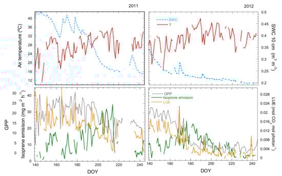
Figure 1.
Seasonal variation of air temperature (T), SWC, GPP, isoprene emissions and LUE at the MOFLUX site in 2011 and 2012.
The seasonal pattern of isoprene emission differed between the two years due to the marked differences in water availability. Isoprene fluxes increased in 2011 from the beginning of May to a peak at the end of July (around DOY 214) and then decreased. Isoprene emissions peaked a few weeks earlier in 2012, at the end of June (DOY 175) (Figure 1). High isoprene emissions were concurrent with the droughts in 2011 (moderate) and 2012 (more severe).
The temporal patterns of isoprene emission, temperature and LUE described two scenarios in both years. Isoprene emissions initially increased to a maximum (increasing phase) as temperature increased and GPP and LUE decreased. Emissions then began to decrease (decreasing phase) when GPP and LUE remained low. Temperature decreased concurrently with emissions in 2011, but temperature began to decrease later than emissions in 2012. Emissions in the decreasing phase were decoupled from LUE in both years and also from temperature in 2012 (Figure 1).
3.2. Influence of Temperature, LUE and SWC on Isoprene Emissions
The patterns of isoprene emission were hierarchically partitioned to measure the importance of the explanatory variables, temperature, LUE and SWC. The independent effects of temperature, LUE and SWC predictors were statistically significant in both years (Figure 2). These variables together explained 88 and 89% of the variance in 2011 and 2012, respectively. Temperature had the highest independent contribution to the total explained variance (48.9% for 2011, 49.4% for 2012), but the contributions of LUE (20.8% for 2011, 31.7% for 2012) and SWC (30.3% for 2011 and 18.9% in 2012) were also important.

Figure 2.
Partial residual plots of the relationships between isoprene emissions and temperature, soil-water content and LUE during the increasing phase of emissions. Shading represents the 95% confidence intervals. β is the standardized regression coefficient.
SWC was highly correlated with both LUE (R2 = 0.60) and PRI (R2 = 0.56). PRI was thus able to detect the effect of low SWC on LUE and thus presumably on isoprene emissions.
3.3. Relationship between Isoprene Emission, LUE and PRI
Isoprene emission was negatively correlated with LUE during the increasing phase (Figure 3). The seasonal pattern of variation in LUE was opposite to that of isoprene emission, peaking on the days with lower emissions and being lower when emission was higher, but only until maximum emission, and then remained low (Figure 1). LUE accounted for 50 and 67% of the variance in isoprene emissions during the increasing phase in 2011 and 2012, respectively (Figure 3). The slope of the relationship was the same in both years (ANCOVA, p > 0.05), but the intercept differed, with a lower emission for the same LUE in 2012.
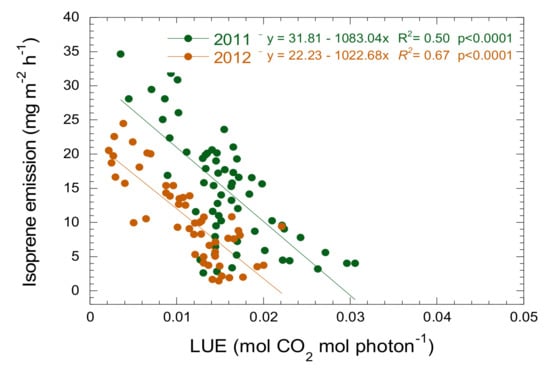
Figure 3.
Relationship between isoprene emissions and LUE at the MOFLUX site during the increasing phase for 2011 and 2012.
PRI varied seasonally in parallel to LUE throughout the entire measurement period (Figure 4). PRI accounted for 52% and 72% of the variance in LUE in 2011 and 2012, respectively. The relationship between LUE and PRI had similar slopes and intercepts in the two years (ANCOVA, p > 0.05).

Figure 4.
Relationship between light-use efficiency (LUE) and the photochemical reflectance index (PRI) at the MOFLUX site for 2011 and 2012.
3.4. Estimation of Isoprene Emissions Using PRI and MEGAN
PRI was significantly and negatively correlated with isoprene emissions during the increasing phase (Figure 5). PRI explained 39 and 63% of the variance in isoprene emissions in 2011 and 2012, respectively. The slope of the relationship was similar (ANCOVA, p > 0.1) for both years but the intercept differed, with lower emission for the same PRI values in 2012.
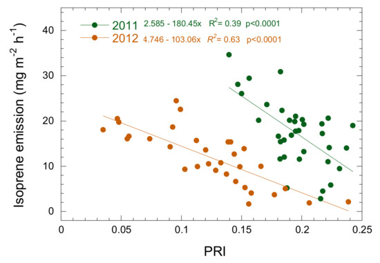
Figure 5.
Relationship between isoprene emission and the photochemical reflectance index (PRI) at the MOFLUX site during the increasing phase in 2011 and 2012.
Midday isoprene flux estimated by the MEGAN model agreed well with the measured emissions (Figure 6), but the model underestimated emissions during the onset of drought conditions in 2011 when the emissions were higher (Figure 6 and Figure 7, [13]), and estimate errors were larger for 2012 when drought conditions were stronger (Figure 6 and Figure 7, [14]). Isoprene emissions were mostly higher than predicted for both 2011 and 2012 after SWC decreased below 0.26 m3 m−3. Emission began to decrease in 2012 when SWC reached the wilting point for this ecosystem (0.23 m3 m−3, [14]), earlier than the MEGAN estimates.
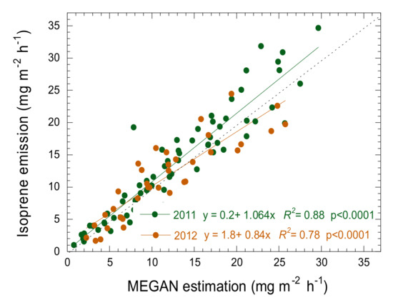
Figure 6.
Relationship between isoprene emission and the results of the isoprene emissions estimated by the MEGAN model for the MOFLUX site during the increasing phase for 2011 and 2012. The dotted line is the 1:1 line.
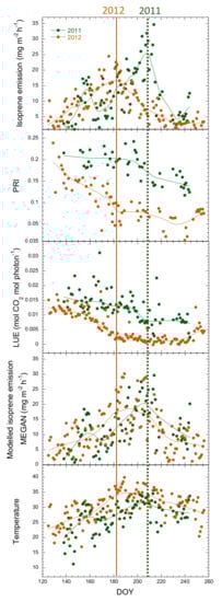
Figure 7.
Comparison of the seasonal variation of isoprene emissions, PRI, LUE, emissions estimated by MEGAN and temperature for 2011 and 2012. The solid lines are spline fits. Vertical dotted lines show the period of maximum isoprene emissions in 2011 and 2012.
The seasonal PRI inflection point in the decreasing phase coincided with the emission peaks in both 2011 and 2012 and was thus sensitive to the advance of the emission peak in 2012. The MEGAN estimates and temperature coincided with the emission peak in 2011 but not 2012, when the measured peak was earlier (Figure 7).
We randomly selected 50% of the data (n = 34) from the increasing phase for both 2011 and 2012 together as a training set for creating two models to estimate isoprenoid emission, one model using MEGAN and another using MEGAN and PRI. The remaining 50% of the data (n = 33) was used for validation. This procedure was repeated 1000 times. Complementing MEGAN algorithms with PRI produced more precise estimates (slopes were 0.89 using MEGAN and 0.98 using MEGAN+PRI) of isoprene emission (Figure 8). Both estimates had the same coefficient of correlation with measured isoprene fluxes, but the model combining MEGAN and PRI was more sensitive to higher emissions, indicated by the better adjustment of the model to the 1:1 line.
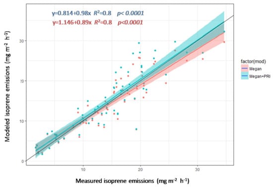
Figure 8.
Measured versus estimated isoprenoid emissions using the MEGAN model and MEGAN model+PRI with data from the increasing phase. The black line is the 1:1 line, and the shading represents the 95% confidence intervals.
4. Discussion
The relationship between isoprene emissions and PRI supported our hypothesis that estimates of isoprenoid emission could be improved by using remotely sensed PRI at the ecosystem level, under conditions of both moderate and extreme drought stress. This capacity of PRI, a good estimator of LUE at foliar, canopy and ecosystem levels [28,29,30,31,54], is based on the inverse relationship between isoprenoid emissions and LUE due to the higher availability of photosynthetic reducing power for isoprenoid production under lower LUEs [25,26,27] and to the positive relationship between PRI (via changes in the xanthophyll cycle and the carotenoid synthesis) and isoprene biosynthesis [25]. Additionally, PRI follows the seasonal change in carotenoid pigment pool sizes (relative to chlorophyll), and these carotenoid pigments are possibly related to isoprene biosynthesis [38,39]. The emission peak of isoprene coincided with an inflection point in the decreasing trend of the LUEs of the vegetation. PRI was sensitive to the isoprene-emission peak coinciding with the drought in 2011, a peak that MEGAN underestimated. PRI was also sensitive to the advance of the emission peak due to severe stress in 2012.
The highest isoprene emissions coinciding with the peak of the drought in 2011 in our study (a decrease in SWC, predawn foliar water potential and net ecosystem production; [13]) were higher than expected due solely to the conditions of light and temperature. This increase in isoprene emissions could be partly due to an increase in foliar temperature caused by drought-induced reductions in stomatal conductance [13,55], but it may also be due to the excess reducing power (Figure 1, DOY 203–215). Isoprene emissions are not well explained by light and temperature under high stress [56,57]. The stimulation of ecosystem isoprene emissions under various abiotic stresses reported in some studies (see references in [11,26,57]) was likely associated with the excess reducing power under stress conditions [17,25]. Residual reducing power not used by carbon assimilation can support increased isoprene emission under drought [58]. LUE explained part of the variance in isoprene emissions (Figure 2), and water stress and LUE were strongly correlated.
Increased emission under drought is sustained if the intensity of drought remains within a species-specific tolerance threshold [59]. Under extreme stress conditions, isoprene emission starts declining for a length of time, which depends on the species studied, until emissions are fully inhibited. Isoprene emission in our study was mostly higher than predicted when SWC was <0.26 m3 m−3, and emission began to decrease when SWC reached the wilting point for this ecosystem (0.23 m3 m−3; [14]). This seasonal decrease occurred earlier in 2012 than 2011 and earlier than modeled. Carbon availability may have critically limited emission under the severe drought at the site in 2012. Water limitation can override the physiological effects of high temperature on isoprene emission during severe stress [60], perhaps due to a very limited amount of recently produced dimethylallyl pyrophosphate (DMAPP), an isoprene substrate [56]. Isoprene is produced in the chloroplast via the methylerythritol phosphate (MEP) pathway [61], which requires both reducing power and carbon skeletons provided by photosynthesis [62]. Bruggemann and Schnitzler [63] attributed the decrease in isoprene emission during drought to a limitation of the carbon supply rather than to a downregulation of isoprene synthase, an enzyme used during isoprene production. PRI was, thus, not as good as an estimator of isoprene emissions later in the season likely because isoprene emissions were decoupled from excess reducing power. The decrease in emissions was likely caused by substrate limitation and lower temperatures in 2011 and by substrate limitation in 2012.
Photosynthesis and isoprene emissions were decoupled seasonally, as previously described under drought conditions (e.g., [13,56,57,60,64,65,66,67,68,69]). Isoprenoid emissions continued to increase concurrently with a decrease in photosynthetic CO2 fixation (GPP) during the increasing phase. Mild stress may decrease carbon assimilation, but isoprene emissions would not be affected, because the rate of electron transport would be maintained and reserve carbon in the form of sugars and starch would support the production of isoprenoids [55]. Isoprene might reduce cell oxidation and increase cell stabilization in plants [70,71], so increasing the allocation of the recently assimilated carbon to isoprene would constitute an additional mechanism of drought resistance [58].
The relationship of PRI with isoprene differed between the two years, as indicated by the different intercepts in the fit (Figure 5). However, the PRI-LUE relationship followed the same regression line for the two years (Figure 4), indicating the good performance of PRI in estimating LUE. The relationship between isoprene emissions and LUE, however, was year-dependent even though the slopes were similar (Figure 3), suggesting that the proportion of available photosynthetic reducing power for isoprene formation differed between the two years. This difference might have been due to a higher competition between photorespiration and the MEP pathway under drought stress as the rate of photorespiration increases and reducing power and carbon supply for the MEP pathway decrease [55], because carbon availability can limit emission rates under severe drought and photorespiratory stresses [55] and isoprene emission may be regulated by substrate availability [67]. The residual reducing power not invested in carbon assimilation is shared by non-photosynthetic sinks such as photorespiration or the MEP pathway [55], and isoprene emission may be most strongly influenced by pathways co-located with the MEP pathway in the chloroplast, such as photorespiration, because they compete directly for both reducing power and photosynthetic carbon [59].
In summary, we hypothesize that seasonal isoprene emissions would be primarily driven by temperature but modulated by reducing power and substrate availability, based on observations and previous conceptual models [13,59]. Photosynthesis, photorespiration and the MEP pathway directly depend on reducing power and substrate availability. The availability of reducing power and substrate for the MEP pathway is thus dependent on photosynthesis and photorespiration. Isoprene emission would thus be stimulated by an increase in available reducing power when drought conditions decrease photosynthesis but would begin to decrease later in the season, despite the high availability of reducing power, because temperature would begin to decrease and substrate would become limiting. Photorespiration increases under drought conditions, causing a decrease in isoprene emissions, and photosynthesis (GPP) becomes minimal under severe drought, so the carbon supply for the MEP pathway is exhausted earlier, advancing the seasonal decrease in isoprene emissions. We summarize the feedbacks involved in the proposed conceptual model in Figure 9. Accordingly, we also propose a model of the performance of PRI and isoprene emissions throughout the season including the final decoupling between them (Figure 10). PRI is highly correlated with isoprene emissions at the beginning of the season and can thus be used to estimate them. Emissions and LUE become decoupled at the end of the season, when LUE (GPP) is lowest and stabilizes; LUE remains low and isoprene emissions begin to decrease.
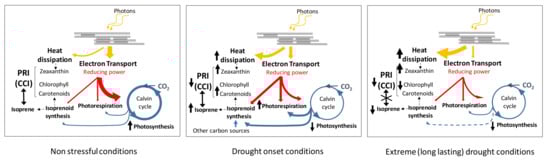
Figure 9.
Schematics of the processes involved in the proposed conceptual model. The yellow arrows indicate the two pathways of energy absorbed by the photosystem involved in the model, electron transport and heat dissipation. The red arrows indicate the flux of reducing power. The blue arrows indicate the flux of carbon. Changes in flux intensities in situations are symbolically represented by changes in arrow width. Upward (downward) arrows indicate increases (decreases). The double pointed arrow indicates correlation between isoprene and PRI (CCI). These schematics are illustrative only and the arrows are not fitted to scale. The scheme does not include the effect of temperature that is one of the main drivers of isoprene emissions.
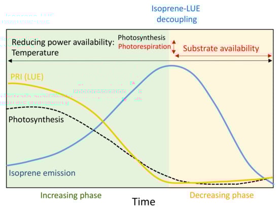
Figure 10.
Conceptual model of the seasonal behavior of PRI and isoprene emissions, with the main drivers that affect their relationship. The variables in red affect isoprene emissions independently of LUE and thus alter the ability of PRI to estimate isoprene emissions.
The effect of photorespiration on the relationship between LUE and isoprene emissions under severe drought conditions can likely disturb the ability of PRI to estimate isoprene emission and can prevent the standardization of the PRI signal, even for the same species or the same ecosystem. The lack of correlation between emissions and LUE late in the season also hinders the use of PRI as a unique estimator for the entire season. Additionally, PRI measured from satellite data represents conditions at the top of canopies, but estimates of GPP using eddy covariance are integrated over the entire canopy [50], which, together with the scatter of eddy covariance measurements, could account for some of the unexplained variability in the LUE-PRI relationship.
PRI, however, was more sensitive than the MEGAN model to temporal changes in isoprene emissions, because it followed changes in LUE, so PRI could be used to improve MEGAN, consistent with previous foliar level studies where PRI combined with basal emission factors was as good a predictor of isoprenoid emissions as some standard emission models and where a combination of MEGAN and PRI provided the best predictions [24]. PRI was thus accounting for additional residual variance not explained by the factors considered in MEGAN. Furthermore, the high temporal resolution and spatially extensive nature of remotely sensed data can help the detection of some of the spatial and temporal variability in emissions that other models may miss [24].
In addition to the diurnal relationship between PRI and LUE mediated by the xanthophyll cycle and indicating excess reducing power, seasonal changes in PRI are primarily influenced by carotenoid pool sizes (relative to chlorophyll). The relationship between PRI and isoprene emissions is strongly influenced by these constitutive changes in pigments [38], so understanding how the isoprene-PRI relationship is affected by both long-term changes in pools of carotenoid pigments and short-term dynamic adjustments of LUE is important in studies with seasonal temporal scales. MODIS PRI (CCI) has been developed to assess shifts in the levels of chlorophyll and carotenoid pigments rather than the xanthophyll de-epoxidation cycle per se, particularly when sampled over seasonal cycles in coniferous forests [37]. Knowledge of the long-term pigment changes would add information for their effect on isoprene emission, facilitating the interpretation of PRI for monitoring isoprene emissions.
5. Conclusions
This study demonstrates that a MODIS PRI (also called CCI), sensitive to carotenoid and chlorophyll pool sizes, could be used to remotely assess isoprene emissions at the ecosystem level.
Complementing MEGAN with PRI improved MEGAN performance under drought conditions. PRI was able to estimate isoprene emissions under standard and drought conditions, but only until emissions reached their maxima. The subsequent decrease in isoprene emissions, likely related to the lack of carbon substrates instead of reducing power, was not well assessed by PRI.
Direct estimation of isoprene emission by PRI is limited because PRI estimates LUE, and the relationship between LUE and isoprene emissions can be modified by stress conditions. Further research is thus needed to resolve this limitation. Additionally, further research is needed to clarify the individual roles of xanthophyll cycle pigments versus other carotenoid pigments in the PRI signals linked to isoprene emissions.
Acknowledgments
This research was supported by the European Research Council Synergy grant SyG-2013-610028 IMBALANCE-P, the Spanish Government project CGL2016-79835-P and the Catalan Government project SGR 2014-274. Chao Zhang gratefully acknowledges the support from the Chinese Scholarship Council. Manuela Balzarolo acknowledges the support provided by the HYPI project funded by BELSPO (Belgian Science Policy Office) in the framework of the STEREO III programme (project HYPI (SR/00/322)) and the support provided by the European Union’s Horizon 2020 research and innovation programme under the Marie Skłodowska-Curie grant agreement No. 76108—INDRO.
Author Contributions
I.F. and J.P. conceived and designed the study; all coauthors were involved in the experiments; I.F. analyzed the data with help of all the coauthors; I.F. drafted the paper and all coauthors contributed to the final writing.
Conflicts of Interest
The authors declare no conflict of interest.
References
- Penuelas, J.; Llusia, J. BVOCs: Plant defense against climate warming? Trends Plant Sci. 2003, 8, 105–109. [Google Scholar] [CrossRef]
- Chameides, W.L.; Lindsay, R.W.; Richardson, J.; Kiang, C.S. The Role of Biogenic Hydrocarbons in Urban Photochemical Smog—Atlanta as a Case-Study. Science 1988, 241, 1473–1475. [Google Scholar] [CrossRef] [PubMed]
- Fuentes, J.D.; Lerdau, M.; Atkinson, R.; Baldocchi, D.; Bottenheim, J.W.; Ciccioli, P.; Lamb, B.; Geron, C.; Gu, L.; Guenther, A.; et al. Biogenic Hydrocarbons in the Atmospheric Boundary Layer: A Review. Bull. Am. Meteorol. Soc. 2000, 81, 1537–1575. [Google Scholar] [CrossRef]
- Andreae, M.O. Atmospheric Aerosols: Biogeochemical Sources and Role in Atmospheric Chemistry. Science 1997, 276, 1052–1058. [Google Scholar] [CrossRef]
- Penuelas, J.; Staudt, M. BVOCs and global change. Trends Plant Sci. 2010, 15, 133–144. [Google Scholar] [CrossRef] [PubMed]
- Westberg, H.; Lamb, B.; Hafer, R.; Hills, A.; Shepson, P.; Vogel, C. Measurement of isoprene fluxes at the PROPHET site. J. Geophys. Res. 2001, 106, 24347–24358. [Google Scholar] [CrossRef]
- Spirig, C.; Neftel, A.; Ammann, C.; Dommen, J.; Grabmer, W.; Thielmann, A.; Schaub, A.; Beauchamp, J.; Wisthaler, A.; Hansel, A. Eddy covariance flux measurements of biogenic VOCs during ECHO 2003 using proton transfer reaction mass spectrometry. Atmos. Chem. Phys. 2005, 5, 465–481. [Google Scholar] [CrossRef]
- Gu, D.; Guenther, A.B.; Shilling, J.E.; Yu, H.; Huang, M.; Zhao, C.; Yang, Q.; Martin, S.T.; Artaxo, P.; Kim, S.; et al. Airborne observations reveal elevational gradient in tropical forest isoprene emissions. Nat. Commun. 2017, 8, 15541. [Google Scholar] [CrossRef] [PubMed]
- Guenther, A.B.; Jiang, X.; Heald, C.L.; Sakulyanontvittaya, T.; Duhl, T.; Emmons, L.K.; Wang, X. The Model of Emissions of Gases and Aerosols from Nature version 2.1 (MEGAN2.1): An extended and updated framework for modeling biogenic emissions. Geosci. Model Dev. 2012, 5, 1471–1492. [Google Scholar] [CrossRef]
- Guenther, A.B.; Zimmerman, P.R.; Harley, P.C.; Monson, R.K.; Fall, R. Isoprene and Monoterpene Emission Rate Variability—Model Evaluations and Sensitivity Analyses. J. Geophys. Res. 1993, 98, 12609–12617. [Google Scholar] [CrossRef]
- Niinemets, U.; Arneth, A.; Kuhn, U.; Monson, R.K.; Penuelas, J.; Staudt, M. The emission factor of volatile isoprenoids: Stress, acclimation, and developmental responses. Biogeosciences 2010, 7, 2203–2223. [Google Scholar] [CrossRef]
- Niinemets, U.; Monson, R.K.; Arneth, A.; Ciccioli, P.; Kesselmeier, J.; Kuhn, U.; Noe, S.M.; Penuelas, J.; Staudt, M. The leaf-level emission factor of volatile isoprenoids: Caveats, model algorithms, response shapes and scaling. Biogeosciences 2010, 7, 1809–1832. [Google Scholar] [CrossRef]
- Potosnak, M.J.; LeStourgeon, L.; Pallardy, S.G.; Hosman, K.P.; Gu, L.; Karl, T.; Geron, C.; Guenther, A.B. Observed and modeled ecosystem isoprene fluxes from an oak-dominated temperate forest and the influence of drought stress. Atmos. Environ. 2014, 84, 314–322. [Google Scholar] [CrossRef]
- Seco, R.; Karl, T.; Guenther, A.; Hosman, K.P.; Pallardy, S.G.; Gu, L.; Geron, C.; Harley, P.; Kim, S. Ecosystem-scale volatile organic compound fluxes during an extreme drought in a broadleaf temperate forest of the Missouri Ozarks (central USA). Glob. Chang. Biol. 2015, 21, 3657–3674. [Google Scholar] [CrossRef] [PubMed]
- IPCC. Climate Change 2014: Impacts, Adaptation, and Vulnerability. Part A: Global and Sectoral Aspects. Contribution of Working Group II to the Fifth Assessment Report of the Intergovernmental Panel on Climate Change, Field, C.B., Barros, V.R., Dokken, D.J., Mach, K.J., Mastrandrea, M.D., Bilir, T.E., Chatterjee, M., Ebi, K.L., Estrada, Y.O., Genova, R.C., et al., Eds.; Cambridge University Press: Cambridge, UK, 2014.
- Monson, R.K.; Grote, R.; Niinemets, U.; Schnitzler, J.-P. Modeling the isoprene emission rate from leaves. New Phytol. 2012, 195, 541–559. [Google Scholar] [CrossRef] [PubMed]
- Morfopoulos, C.; Prentice, I.C.; Keenan, T.F.; Friedlingstein, P.; Medlyn, B.E.; Penuelas, J.; Possell, M. A unifying conceptual model for the environmental responses of isoprene emissions from plants. Ann. Bot. 2013, 112, 1223–1238. [Google Scholar] [CrossRef] [PubMed]
- Niinemets, U.; Tenhunen, J.D.; Harley, P.C.; Steinbrecher, R. A model of isoprene emission based on energetic requirements for isoprene synthesis and leaf photosynthetic properties for Liquidambar and Quercus. Plant Cell Environ. 1999, 22, 1319–1335. [Google Scholar] [CrossRef]
- Grote, R.; Morfopoulos, C.; Niinemets, U.; Sun, Z.; Keenan, T.F.; Pacifico, F.; Butler, T. A fully integrated isoprenoid emissions model coupling emissions to photosynthetic characteristics. Plant Cell Environ. 2014, 37, 1965–1980. [Google Scholar] [CrossRef] [PubMed]
- Palmer, P.I.; Jacob, D.J.; Fiore, A.M.; Martin, R.V.; Chance, K.; Kurosu, T.P. Mapping isoprene emissions over North America using formaldehyde column observations from space. J. Geophys. Res. 2003, 108. [Google Scholar] [CrossRef]
- Barkley, M.P.; Palmer, P.I.; Kuhn, U.; Kesselmeier, J.; Chance, K.; Kurosu, T.P.; Martin, R.V.; Helmig, D.; Guenther, A. Net ecosystem fluxes of isoprene over tropical South America inferred from Global Ozone Monitoring Experiment (GOME) observations of HCHO columns. J. Geophys. Res. 2008, 113. [Google Scholar] [CrossRef]
- Foster, P.N.; Prentice, I.C.; Morfopoulos, C.; Siddall, M.; van Weele, M. Isoprene emissions track the seasonal cycle of canopy temperature, not primary production: Evidence from remote sensing. Biogeosciences 2014, 11, 3437–3451. [Google Scholar] [CrossRef]
- Valin, L.C.; Fiore, A.M.; Chance, K.; Abad, G.G. The role of OH production in interpreting the variability of CH2O columns in the southeast U.S. J. Geophys. Res. Atmos. 2016, 478–493. [Google Scholar] [CrossRef]
- Penuelas, J.; Marino, G.; Llusia, J.; Morfopoulos, C.; Farre-Armengol, G.; Filella, I. Photochemical reflectance index as an indirect estimator of foliar isoprenoid emissions at the ecosystem level. Nat. Commun. 2013, 4. [Google Scholar] [CrossRef] [PubMed]
- Morfopoulos, C.; Sperlich, D.; Penuelas, J.; Filella, I.; Llusia, J.; Medlyn, B.E.; Niinemets, U.; Possell, M.; Sun, Z.; Prentice, I.C. A model of plant isoprene emission based on available reducing power captures responses to atmospheric CO2. New Phytol. 2014, 203, 125–139. [Google Scholar] [CrossRef] [PubMed]
- Penuelas, J.; Llusia, J. Plant VOC emissions: Making use of the unavoidable. Trends Ecol. Evol. 2004, 19, 402–404. [Google Scholar] [CrossRef] [PubMed]
- Owen, S.M.; Penuelas, J. Opportunistic emissions of volatile isoprenoids. Trends Plant Sci. 2005, 10, 420–426. [Google Scholar] [CrossRef] [PubMed]
- Penuelas, J.; Garbulsky, M.F.; Filella, I. Photochemical reflectance index (PRI) and remote sensing of plant CO2 uptake. New Phytol. 2011, 191, 596–599. [Google Scholar] [CrossRef] [PubMed]
- Zhang, C.; Filella, I.; Garbulsky, M.F.; Peñuelas, J. Affecting Factors and Recent Improvements of the Photochemical Reflectance Index (PRI) for Remotely Sensing Foliar, Canopy and Ecosystemic Radiation-Use Efficiencies. Remote Sens. 2016, 8, 677. [Google Scholar] [CrossRef]
- Penuelas, J.; Filella, I.; Gamon, J.A. Assessment of Photosynthetic Radiation-Use Efficiency with Spectral Reflectance. New Phytol. 1995, 131, 291–296. [Google Scholar] [CrossRef]
- Gamon, J.A.; Penuelas, J.; Field, C.B. A Narrow-Waveband Spectral Index That Tracks Diurnal Changes in Photosynthetic Efficiency. Remote Sens. Environ. 1992, 41, 35–44. [Google Scholar] [CrossRef]
- Sims, D.A.; Gamon, J.A. Relationships between leaf pigment content and spectral reflectance across a wide range of species, leaf structures and developmental stages. Remote Sens. Environ. 2002, 81, 337–354. [Google Scholar] [CrossRef]
- Stylinski, C.D.; Gamon, J.A.; Oechel, W.C. Seasonal patterns of reflectance indices, carotenoid pigments and photosynthesis of evergreen chaparral species. Oecologia 2002, 131, 366–374. [Google Scholar] [CrossRef] [PubMed]
- Filella, I.; Porcar-Castell, A.; Munne-Bosch, S.; Back, J.; Garbulsky, M.F.; Penuelas, J. PRI assessment of long-term changes in carotenoids/chlorophyll ratio and short-term changes in de-epoxidation state of the xanthophyll cycle. Int. J. Remote Sens. 2009, 30, 4443–4455. [Google Scholar] [CrossRef]
- Porcar-Castell, A.; Ignacio Garcia-Plazaola, J.; Nichol, C.J.; Kolari, P.; Olascoaga, B.; Kuusinen, N.; Fernandez-Marin, B.; Pulkkinen, M.; Juurola, E.; Nikinmaa, E. Physiology of the seasonal relationship between the photochemical reflectance index and photosynthetic light use efficiency. Oecologia 2012, 170, 313–323. [Google Scholar] [CrossRef] [PubMed]
- Wong, C.Y.S.; Gamon, J.A. Three causes of variation in the photochemical reflectance index (PRI) in evergreen conifers. New Phytol. 2015, 206, 187–195. [Google Scholar] [CrossRef] [PubMed]
- Gamon, J.A.; Huemmrich, K.F.; Wong, C.Y.S.; Ensminger, I.; Garrity, S.; Hollinger, D.Y.; Noormets, A.; Peñuelas, J. A remotely sensed pigment index reveals photosynthetic phenology in evergreen conifers. Proc. Natl. Acad. Sci. USA 2016, 113, 13087–13092. [Google Scholar] [CrossRef] [PubMed]
- Harris, A.; Owen, S.M.; Sleep, D.; Pereira, M.D.G.D.S. Constitutive changes in pigment concentrations: Implications for estimating isoprene emissions using the photochemical reflectance index. Physiol. Plant. 2016, 156, 190–200. [Google Scholar] [CrossRef] [PubMed]
- Owen, S.M.; Penuelas, J. Volatile isoprenoid emission potentials are correlated with essential isoprenoid concentrations in five plant species. Acta Physiol. Plant. 2013, 35, 3109–3125. [Google Scholar] [CrossRef]
- Harley, P.C.; Litvak, M.E.; Sharkey, T.D.; Monson, R.K. Isoprene Emission from Velvet Bean Leaves. Plant Physiol. 1994, 105, 279–285. [Google Scholar] [CrossRef] [PubMed]
- Geron, C.; Guenther, A.; Sharkey, T.; Arnts, R.R. Temporal variability in basal isoprene emission factor. Tree Physiol. 2000, 20, 799–805. [Google Scholar] [CrossRef] [PubMed]
- Pressley, S.; Lamb, B.; Westberg, H.; Flaherty, J.; Chen, J.; Vogel, C. Long-term isoprene flux measurements above a northern hardwood forest. J. Geophys. Res. 2005, 110. [Google Scholar] [CrossRef]
- Gu, L.; Meyers, T.; Pallardy, S.G.; Hanson, P.J.; Yang, B.; Heuer, M.; Hosman, K.P.; Riggs, J.S.; Sluss, D.; Wullschleger, S.D. Direct and indirect effects of atmospheric conditions and soil moisture on surface energy partitioning revealed by a prolonged drought at a temperate forest site. J. Geophys. Res. 2006, 111. [Google Scholar] [CrossRef]
- Critchfield, H.J. General Climatology; Prentice-Hall: Englewood Cliffs, NJ, USA, 1966. [Google Scholar]
- Guenther, A.B.; Hills, A.J. Eddy covariance measurement of isoprene fluxes. J. Geophys. Res. 1998, 103, 13145–13152. [Google Scholar] [CrossRef]
- Karl, T.G.; Spirig, C.; Rinne, J.; Stroud, C.; Prevost, P.; Greenberg, J.; Fall, R.; Guenther, A. Virtual disjunct eddy covariance measurements of organic compound fluxes from a subalpine forest using proton transfer reaction mass spectrometry. Atmos. Chem. Phys. 2002, 2, 279–291. [Google Scholar] [CrossRef]
- Reichstein, M.; Falge, E.; Baldocchi, D.; Papale, D.; Aubinet, M.; Berbigier, P.; Bernhofer, C.; Buchmann, N.; Gilmanov, T.; Granier, A.; et al. On the separation of net ecosystem exchange into assimilation and ecosystem respiration: Review and improved algorithm. Glob. Chang. Biol. 2005, 11, 1424–1439. [Google Scholar] [CrossRef]
- Monteith, J.L. Using Tube Solarimeters to Measure Radiation Intercepted by Crop Canopies and to Analyse Stand Growth; Application Note: TSL-AN-4-1; Delta-T Devices: Cambridge, UK, 1993; pp. 1–11. [Google Scholar]
- Rahman, A.F.; Cordova, V.D.; Gamon, J.A.; Schmid, H.P.; Sims, D.A. Potential of MODIS ocean bands for estimating CO2 flux from terrestrial vegetation: A novel approach. Geophys. Res. Lett. 2004, 31. [Google Scholar] [CrossRef]
- Goerner, A.; Reichstein, M.; Rambal, S. Tracking seasonal drought effects on ecosystem light use efficiency with satellite-based PRI in a Mediterranean forest. Remote Sens. Environ. 2009, 113, 1101–1111. [Google Scholar] [CrossRef]
- Mac Nally, R.; Walsh, C.J. Hierarchical partitioning public-domain software. Biodivers. Conserv. 2004, 13, 659–660. [Google Scholar] [CrossRef]
- Breheny, P.; Burchett, W. Visualization of regression models using visreg. R Packag. 2013, 1–15. [Google Scholar]
- R Core Team. R: A Language and Environment for Statistical Computing. R Found. Stat. Comput. 2015, 1, 1651. [Google Scholar]
- Garbulsky, M.F.; Penuelas, J.; Gamon, J.; Inoue, Y.; Filella, I. The photochemical reflectance index (PRI) and the remote sensing of leaf, canopy and ecosystem radiation use efficiencies: A review and meta-analysis. Remote Sens. Environ. 2011, 115, 281–297. [Google Scholar] [CrossRef]
- Niinemets, U. Mild versus severe stress and BVOCs: Thresholds, priming and consequences. Trends Plant Sci. 2010, 15, 145–153. [Google Scholar] [CrossRef] [PubMed]
- Tani, A.; Tozaki, D.; Okumura, M.; Nozoe, S.; Hirano, T. Effect of drought stress on isoprene emission from two major Quercus species native to East Asia. Atmos. Environ. 2011, 45, 6261–6266. [Google Scholar] [CrossRef]
- Genard-Zielinski, A.-C.; Ormeno, E.; Boissard, C.; Fernandez, C. Isoprene Emissions from Downy Oak under Water Limitation during an Entire Growing Season: What Cost for Growth? PLoS ONE 2014, 9. [Google Scholar] [CrossRef] [PubMed]
- Dani, K.G.S.; Jamie, I.M.; Prentice, I.C.; Atwell, B.J. Increased Ratio of Electron Transport to Net Assimilation Rate Supports Elevated Isoprenoid Emission Rate in Eucalypts under Drought. Plant Physiol. 2014, 166, 1059–1072. [Google Scholar] [CrossRef] [PubMed]
- Dani, K.G.S.; Jamie, I.M.; Prentice, I.C.; Atwell, B.J. Species-specific photorespiratory rate, drought tolerance and isoprene emission rate in plants. Plant Signal. Behav. 2015, 10, e990830. [Google Scholar] [CrossRef] [PubMed]
- Fortunati, A.; Barta, C.; Brilli, F.; Centritto, M.; Zimmer, I.; Schnitzler, J.-P.; Loreto, F. Isoprene emission is not temperature-dependent during and after severe drought-stress: A physiological and biochemical analysis. Plant J. 2008, 55, 687–697. [Google Scholar] [CrossRef] [PubMed]
- Li, Z.; Sharkey, T.D. Metabolic profiling of the methylerythritol phosphate pathway reveals the source of post-illumination isoprene burst from leaves. Plant Cell Environ. 2013, 36, 429–437. [Google Scholar] [CrossRef] [PubMed]
- Loreto, F.; Schnitzler, J.-P. Abiotic stresses and induced BVOCs. Trends Plant Sci. 2010, 15, 154–166. [Google Scholar] [CrossRef] [PubMed]
- Poorter, H.; Buehler, J.; van Dusschoten, D.; Climent, J.; Postma, J.A. Pot size matters: A meta-analysis of the effects of rooting volume on plant growth. Funct. Plant Biol. 2012, 39, 839–850. [Google Scholar] [CrossRef]
- Bertin, N.; Staudt, M. Effect of water stress on monoterpene emissions from young potted holm oak (Quercus ilex L.) trees. Oecologia 1996, 107, 456–462. [Google Scholar] [CrossRef] [PubMed]
- Brilli, F.; Barta, C.; Fortunati, A.; Lerdau, M.; Loreto, F.; Centritto, M. Response of isoprene emission and carbon metabolism to drought in white poplar (Populus alba) saplings. New Phytol. 2007, 175, 244–254. [Google Scholar] [CrossRef] [PubMed]
- Funk, J.L.; Jones, C.G.; Gray, D.W.; Throop, H.L.; Hyatt, L.A.; Lerdau, M.T. Variation in isoprene emission from Quercus rubra: Sources, causes, and consequences for estimating fluxes. J. Geophys. Res. 2005, 110. [Google Scholar] [CrossRef]
- Funk, J.L.; Mak, J.E.; Lerdau, M.T. Stress-induced changes in carbon sources for isoprene production in Populus deltoides. Plant Cell Environ. 2004, 27, 747–755. [Google Scholar] [CrossRef]
- Pegoraro, E.; Rey, A.; Greenberg, J.; Harley, P.; Grace, J.; Malhi, Y.; Guenther, A. Effect of drought on isoprene emission rates from leaves of Quercus virginiana Mill. Atmos. Environ. 2004, 38, 6149–6156. [Google Scholar] [CrossRef]
- Wu, C.; Pullinen, I.; Andres, S.; Carriero, G.; Fares, S.; Goldbach, H.; Hacker, L.; Kasal, T.; Kiendler-Scharr, A.; Kleist, E.; et al. Impacts of soil moisture on de novo monoterpene emissions from European beech, Holm oak, Scots pine, and Norway spruce. Biogeosciences 2015, 12, 177–191. [Google Scholar] [CrossRef]
- Sharkey, T.D.; Wiberley, A.E.; Donohue, A.R. Isoprene emission from plants: Why and how. Ann. Bot. 2008, 101, 5–18. [Google Scholar] [CrossRef] [PubMed]
- Velikova, V.; Sharkey, T.D.; Loreto, F. Stabilization of thylakoid membranes in isoprene-emitting plants reduces formation of reactive oxygen species. Plant Signal. Behav. 2012, 7, 139–141. [Google Scholar] [CrossRef] [PubMed]


© 2018 by the authors. Licensee MDPI, Basel, Switzerland. This article is an open access article distributed under the terms and conditions of the Creative Commons Attribution (CC BY) license (http://creativecommons.org/licenses/by/4.0/).