Thaw Subsidence of a Yedoma Landscape in Northern Siberia, Measured In Situ and Estimated from TerraSAR-X Interferometry

Abstract

In permafrost areas, seasonal freeze-thaw cycles result in upward and downward movements of the ground. For some permafrost areas, long-term downward movements were reported during the last decade. We measured seasonal and multi-year ground movements in a yedoma region of the Lena River Delta, Siberia, in 2013–2017, using reference rods installed deep in the permafrost. The seasonal subsidence was 1.7 ± 1.5 cm in the cold summer of 2013 and 4.8 ± 2 cm in the warm summer of 2014. Furthermore, we measured a pronounced multi-year net subsidence of 9.3 ± 5.7 cm from spring 2013 to the end of summer 2017. Importantly, we observed a high spatial variability of subsidence of up to 6 cm across a sub-meter horizontal scale. In summer 2013, we accompanied our field measurements with Differential Synthetic Aperture Radar Interferometry (DInSAR) on repeat-pass TerraSAR-X (TSX) data from the summer of 2013 to detect summer thaw subsidence over the same study area. Interferometry was strongly affected by a fast phase coherence loss, atmospheric artifacts, and possibly the choice of reference point. A cumulative ground movement map, built from a continuous interferogram stack, did not reveal a subsidence on the upland but showed a distinct subsidence of up to 2 cm in most of the thermokarst basins. There, the spatial pattern of DInSAR-measured subsidence corresponded well with relative surface wetness identified with the near infra-red band of a high-resolution optical image. Our study suggests that (i) although X-band SAR has serious limitations for ground movement monitoring in permafrost landscapes, it can provide valuable information for specific environments like thermokarst basins, and (ii) due to the high sub-pixel spatial variability of ground movements, a validation scheme needs to be developed and implemented for future DInSAR studies in permafrost environments.

1. Introduction

In the Northern Hemisphere, permafrost occupies up to 18% of the land area [1], and its depth reaches up to 1500 m below the land surface in particular areas of Eastern Siberia [2]. In permafrost regions, the active layer is the upper layer of the ground that thaws and freezes seasonally. Active layer thawing typically takes a few months, starting when the surface becomes free of snow in spring and ending when freezing begins in the fall. An active layer, which is water-saturated in summer, increases in volume during freezing in winter. This occurs due to the increase in volume of ice compared to water in ground material pores (about 9% for fresh water). Besides the water-ice phase change in pore ice, in fine-grained sediments, the cryosuction causes migration of the liquid water to the freezing front, leading to the formation of segregated ice lenses. The power of segregated ice growth forces the overlying frozen soil to heave (e.g., [3]). Thawing season sees the melting of both the excess ice in soil pores and the segregated ice. Subsequently, the decrease of the volume due to the phase change and the outward flow of the melt water cause the soil to settle. Thus, cycles of freezing and thawing in the active layer result in seasonal vertical movements of the ground surface in both directions, i.e., uplift and settlement or subsidence. The magnitude of these movements largely depends on the ice/water content and its distribution in the active layer. Measuring the magnitudes of these movements can, in turn, be used to estimate the ice/water content, which is one of the most important ground variables for permafrost modeling [4].

Shiklomanov et al. [5] introduce the term “isotropic thaw subsidence” for a phenomenon of relatively uniform and long-term thawing of the ice-rich layer typically found directly beneath the active layer. Isotropic thaw subsidence is, thus, different from rather rapid and spatially confined thermokarst or thaw slump ground subsidence and, unlike them, does not feature any apparent terrain disturbance. The above authors show that, due to such isotropic subsidence, the record of active layer thickness in Alaska does not demonstrate a clear increasing trend, which was expected as a result of the effect of atmospheric warming in the Arctic. Accounting for the isotropic subsidence is, therefore, necessary to accurately represent long-term active layer thickness dynamics.

Reported in situ measurements on seasonal and long-term subsidence and uplift in permafrost areas include repeated differential global positioning system (DGPS) measurements of the ground surface elevation (e.g., [5,6,7,8]), Linear Variable Differential Transformer (LVDT)-based measurements (e.g., [9,10]), and thaw-tubes (e.g., [11,12,13]). Field campaigns to install equipment and conduct measurements are expensive and do not provide good spatial coverage. However, such measurements provide the most reliable information on ground motion and are important for remote sensing validation.

Detecting and quantifying ground uplift and subsidence over permafrost regions by using remote sensing methods is advantageous due to large spatial coverage and potential avoidance of expensive field campaigns. Related methods include differencing of multitemporal Digital Elevation Models (DEMs) (e.g., [14]) and repeat-pass differential SAR (Synthetic Aperture Radar) interferometry (DInSAR). The former technique generally can only be applied to monitor ground motion which is larger than DEM vertical accuracy, and thus is suitable for measuring only multiyear ground motion. The latter technique is more sensitive to small-scale ground motion. It uses the phase difference between two radar signals acquired on two dates over the same area to measure ground displacement. It is applied widely and successfully for detecting ground displacement associated with earthquakes, volcanic eruptions, urban development, and mining activities. During the last decade the method has been adapted for monitoring permafrost-related ground motion. A number of studies report a centimeter- to decimeter-scale seasonal and multiyear isotropic thaw subsidence in permafrost areas derived with DInSAR (e.g., [12,13,15,16,17,18]). These studies were, however, not validated by ground-truth measurements or were limited to a few point measurements performed with thaw-tubes. Short et al. [18] raise the problem of comparison pointwise in situ and areal DInSAR measurements, and fairly suggest that agreement between them might never be achieved. So far, approaches to adequately validate DInSAR results in permafrost areas have not been proposed.

Besides the validation problem, the DInSAR method itself has some serious limitations. The interferometric phase decorrelates for surfaces that change through time, which causes a loss of interferometric signal. This phase decorrelation (or coherence loss) generally increases with shorter radar wavelength (such as X-band with a wavelength of approximately 3 cm) and with increasing time period spanned by the interferograms. Thus, a few studies demonstrate a limited suitability of TerraSAR-X (TSX) data for the interferometric analysis of permafrost dynamics in the Canadian Arctic and subarctic due to low phase coherence and show the advantages of using C- and L-band (e.g., [7,13,18]). However, the longer waves can be more sensitive to the soil moisture changes between SAR acquisitions due to potentially deeper penetration into the ground, causing larger errors in displacement estimations (e.g., [19]). Another potential problem for DInSAR is a non-uniform distribution of water/ice in the ground, which leads to heterogeneous uplift/subsidence within a DInSAR resolution cell. Zwieback et al. [20] show that the multiple scatterers with variable phase contribution in a resolution cell can result not only in phase decorrelation but also in systematic errors influencing the accuracy or even validity of the DInSAR ground movement estimations.

TSX data have the advantage of high spatial resolution (up to 2.5 m) and relatively short revisit time (11 days) which can partly compensate for temporal decorrelation. A precursory study of interferometric coherence time series of TSX data in the Lena River Delta, Siberia demonstrated the large spatial and temporal variability of 11-day sequential coherence during one year, 2012–2013 [21]. Some single interferograms showed sufficient coherence to test their potential for DInSAR analysis. Here we perform DInSAR on a subset of the same TSX data to assess viability for thaw subsidence detection in a yedoma landscape of the Lena River Delta. DInSAR results are accompanied by field measurements made between 2013 and 2017. We discuss the sub-pixel variability of the ground movement and its implications for the DInSAR errors and validation. Furthermore, we compare the DInSAR results with the surface wetness spatial distribution estimated from the near infra-red band of a high-resolution optical image.

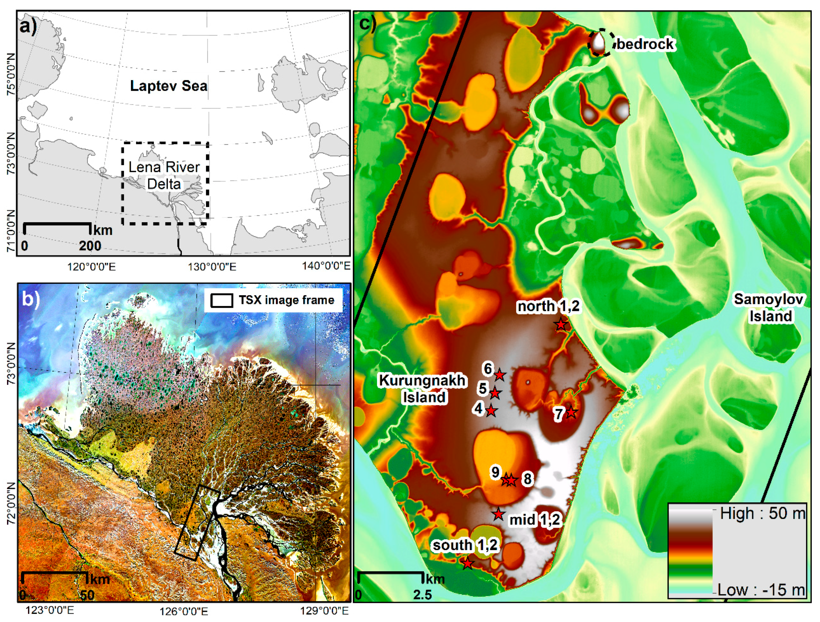
2. Study Area

The Siberian Lena River Delta (73°N; 126°E) comprises more than 1500 islands of various sizes and has an area of about 30,000 km² (Figure 1a,b). It is located in the zone of continuous permafrost, with permafrost depth reaching up to 600 m [22]. The climate of the region is generally characterized by long, extremely cold winters and short, cool summers, with mean February temperatures of −33.1 °C and mean July temperatures of 10.1 °C over the last decade [23]. The absence of glaciation during the Pleistocene as well as cold air temperatures in the past and present result in low permafrost temperatures compared, for instance, to Svalbard or Alaska, with temperatures of about −9 °C at the depth of zero annual amplitude [24]. Snow accumulation typically begins in September; snow melt begins in May, and snow usually melts completely in less than a month. Snow depth is highly variable due to microtopography and wind redistribution, but generally does not exceed a few decimeters. The active layer usually begins to thaw in the first half of June, reaching an average maximum thickness of about 50 cm. Active layer freezing commences with the onset of negative air temperatures and is usually complete in November [23].

We focused in particular on Kurungnakh-Sise Island in the southern part of the delta, which largely represents the remnants of a late Pleistocene accumulation plain (Figure 1b,c). Stratigraphically, the island consists of 15–20 m thick fluvial silty sands overlain by up to 40 m thick ice-rich peaty and silty deposits, also known as yedoma or Ice Complex. The ground ice in these deposits occurs in the form of small ice veins and lenses as well as giant ice wedges, which can reach up to 20 m high and several meters wide. The Holocene layer on the very top can be as thin as 0.5 m and features peaty soils interbedded with silty sands (e.g., [25,26,27]).

The relief of the island is largely a result of permafrost degradation processes that started in the mid-Holocene and is characterized by thermo-erosional valleys and thermokarst basins, which occupy about 40% of the island area. The upland is characterized by poorly developed polygonal tundra with small ponds and thermokarst lakes. The maximum relief height of the island is 55 m a.s.l. and the mean elevation gradually decreases from southeast to northwest, which has led to the development of a drainage network [28]. Relict bedrock islands with elevations of about 60 m are present in the area as well (Figure 1c). The region is characterized by typical tundra vegetation, which includes sedges, grasses, dwarf shrubs, and a well-developed moss layer.

We chose this island of non-deltaic origin for the analysis because of its relatively homogenous surface compared to the other parts of the delta, which are characterized by abundant thermokarst lakes and ponds, floodplains, and distinct polygonal tundra.

3. Data and Methods

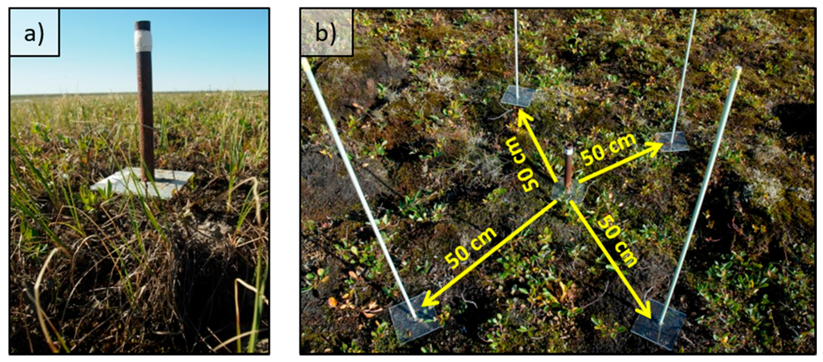
3.1. Field Measurements of Surface Displacement

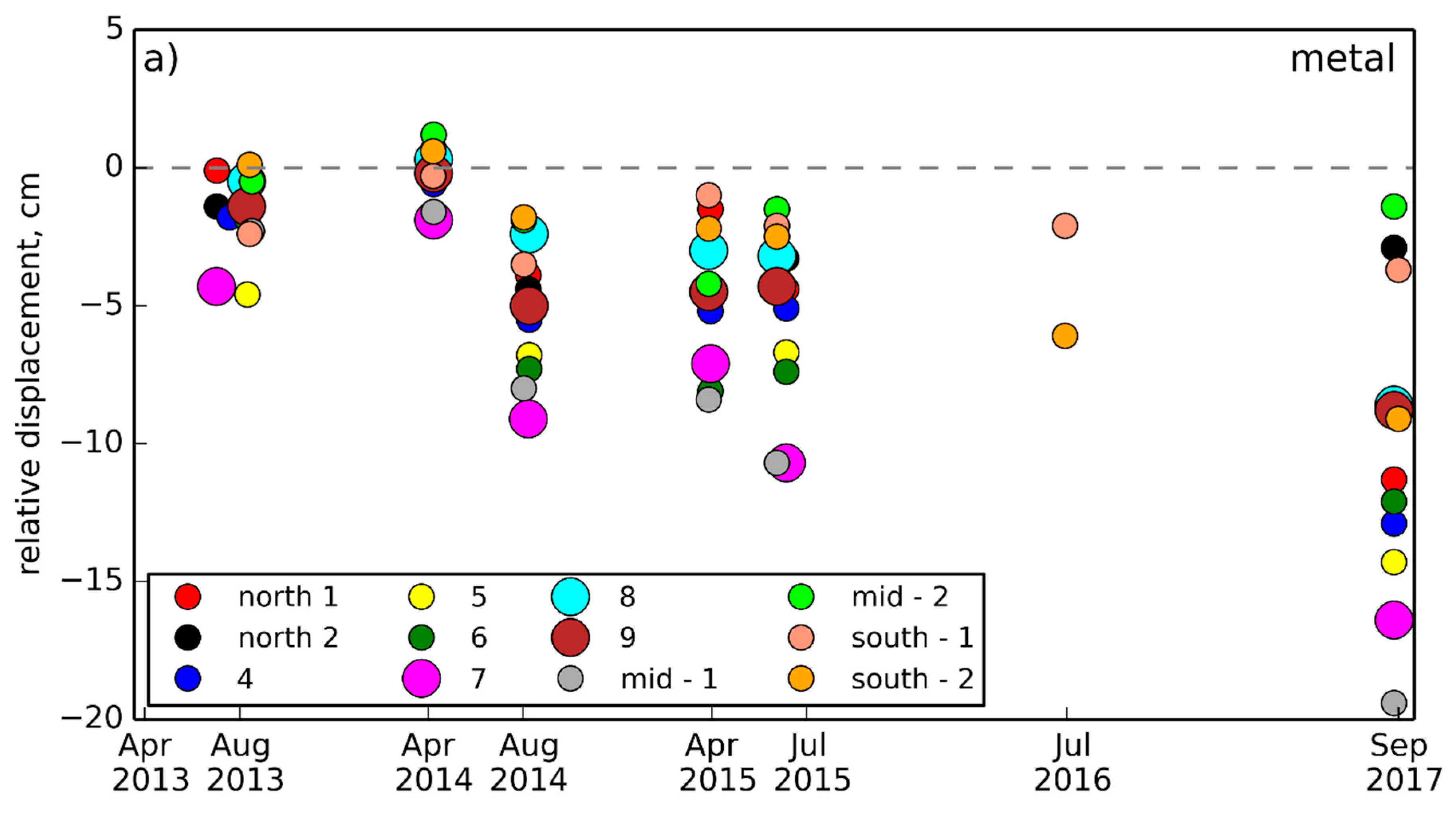
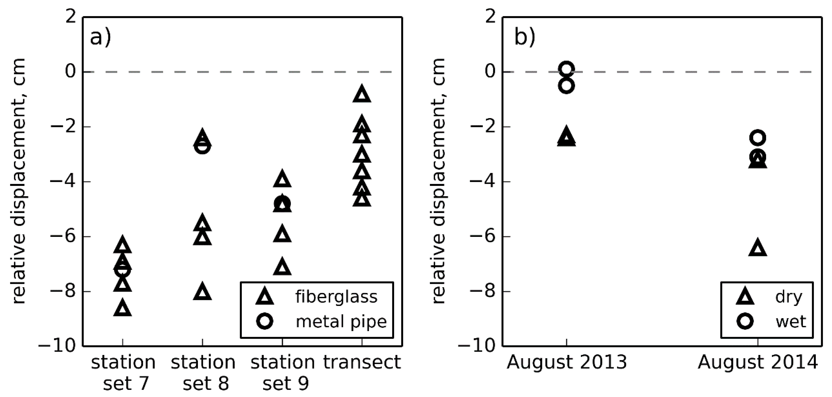
3.1.1. Metal Pipes (2013–2017)

Surface displacement was determined by repeatedly measuring the distance between the top of a steel pipe and a plexiglass plate resting on the ground surface (Figure 2a). The pipe was 2 m long and 3 cm in diameter and was anchored at least 1 m below the active layer. We assume, therefore, that the pipe was motionless relative to the permafrost. The plexiglass plate with a size of 10 by 10 cm was fixed in its horizontal position by the metal pipe but could move freely with the surface vertically along the pipe. Several distance measurements around the pipe were taken at each visit and averaged. Altogether 12 metal pipes were installed at the study site in April 2013 (Figure 1c). Measurements were conducted during field campaigns from spring 2013 to summer 2017 with some gaps (

Table 1. Periods of field measurements.

	Spring 2013	Summer 2013	Spring 2014	Summer 2014	Spring 2015	Summer 2015	Spring 2016	Summer 2016	Spring 2017	Summer 2017
metal pipes	25–30 April	irregularly during July and August	22 April	5–7 August and 22–23 August	11 April	8–20 July	-	-	-	9–15 September
fiberglass poles	-	-	22 April	5–7 August and 22–23 August	11 April	8–20 July	-	-	-	9–15 September

).

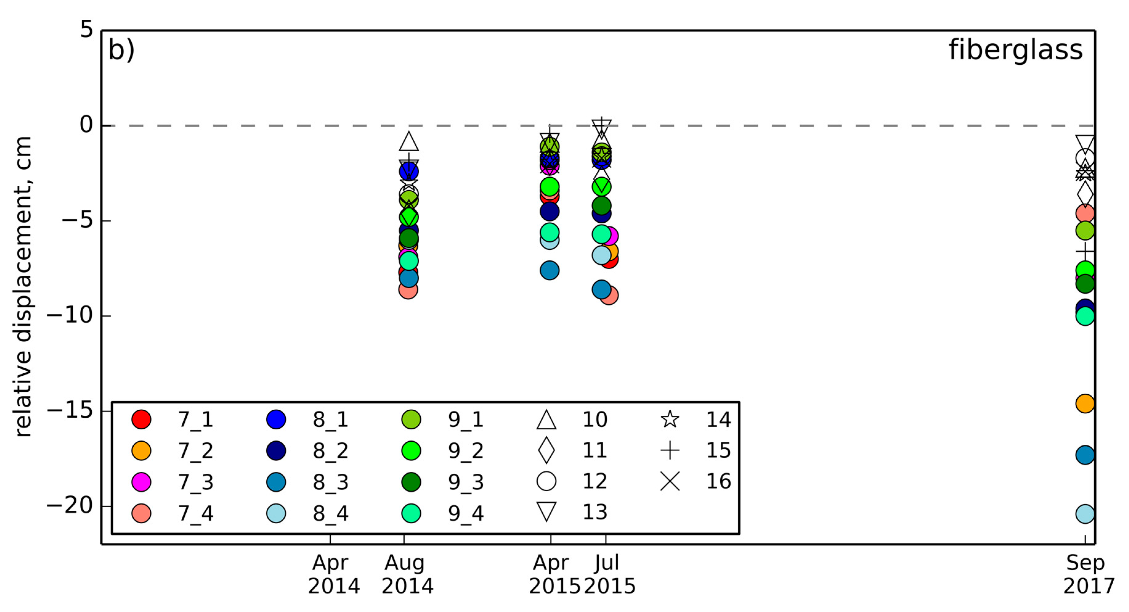
3.1.2. Fiberglass Poles (2014–2017)

Nineteen fiberglass poles, 2 m long and 1 cm in diameter, were installed in spring 2014. Following the method for the metal pipes, the poles were anchored at least 70 cm into the permafrost and were outfitted with plexiglass plates. To explore the small-scale spatial variability of ground displacements and to compare the effect of two different materials, these poles were installed near the locations of metal pipes. Four fiberglass poles were added around each of the metal pipe 7, 8, and 9 (e.g., Figure 2b). The radius between metal pipe 7 and fiberglass poles was 1 m, and the radius between metal pipes 8 and 9 and their fiberglass poles was 50 cm. In addition, a transect of seven fiberglass poles was installed between metal pipes 8 and 9, with approximately 25 m intervals between fiberglass poles. Measurements were conducted during field campaigns from spring 2014 to summer 2017 with some gaps (Table 1).

3.1.3. Sources of Potential Errors in Field Measurements

Installation of metal pipes and fiberglass poles (both hereinafter referred to as “reference rods”) via deep drilling could have affected the state of permafrost and active layer to some extent. Moreover, the high thermal conductivity of metal could potentially induce additional warming and cooling of the ground. However, visual inspection of the measurement sites did not reveal any drastic changes (e.g., water ponding) of the tundra surface around the rods up to the summer season in 2017. Therefore, we assume no significant and systematic error source in the measurement setup. No difference between the steel and fiberglass sites were observed, although they differ significantly in thermal conductivity (40 and 0.04 W/mK, respectively).

Other potential uncertainties are inherent in the method used to obtain manual distance measurements. For example, the pressure exerted to push a plexiglass plate down into a vegetation and moss layer can differ; this is hard to control. Moreover, the presence of vegetation under the plate is itself an additional source of error, especially in the case of vascular plants, which can grow under the plate, lifting it up seasonally to some extent. Overall, we assume ±1 cm as a reasonable measurement uncertainty.

A very important source of erroneous measurements is potential upward heaving of the rods despite the rods being anchored in permafrost. If that were the case, any increased distance between the top of the rod and the ground surface could simply represent the degree to which the rod has been expelled rather than the degree to which the ground has subsided. We address this problem by calculating the balance between the heaving force and the resistance force which grips the rod in permafrost. According to the Russian building code [29], the heaving force can be calculated by

$$F_h=\pi d{h}_{AL}·{\tau }_{fh}$$

(1)

where $d$ is the diameter of the rod, $h_{AL}$ is the active layer thickness and ${\tau }_{fh}$ is the tangential adfreezing strength (TAS), which characterizes the bond between the surface of the rod and the frozen ground. The TAS depends on ground texture, moisture content, and temperature as well as the material of the rod. Laboratory experiments are typically used to determine the TAS. Therefore, it is problematic to find reliable quantitative data concerning the variety of influencing parameters. We use the table values from the building code which are provided for different soil types and for the active layer depths from 1 to 3 m. We extrapolate values for the typical active layer depth in our study area which typically does not exceed 40 cm. The obtained TAS values vary from 0.57 to 0.99 kgf/cm² (57 to 99 kPa) for different soil types. Therefore, the heaving force on the 3 cm diameter steel pipe is in the range from 215 to 377 kgf and the heaving force on the 1 cm diameter fiberglass pole is in the range from 71.6 to 125.6 kgf.

According to the same building code, the force which grips the rod in the permafrost beneath the active layer can be calculated by

$$F_r=\pi d(h-h_{AL})·R_{af}$$

(2)

where $h$ is depth at which the rod is anchored and $R_{af}$ is the shear resistance of the frozen ground along the adfreezing surface. The latter is also given in the building code for different soil types and ground temperatures. Wetterich et al. [27] report an organic content of 3–12 wt% within the upper permafrost layer at our study site. The ground temperatures at the depth of 75 cm at the long-term observatory on Samoylov Island (approximately 10 km from the study site, see Figure 1c) are around −2 °C during the freezing period ([23], updated dataset). Corresponding table values for the sandy and silty-clayed biogenic soils are 1.3 and 1 kgf/cm² respectively. Thus, the resistance force which retains the metal pipe in permafrost ranges from 1225 to 1592 kgf and the resistance force which retains the fiberglass pole in permafrost ranges from 235 to 306 kgf.

The resistance forces are, therefore, two to seven times larger than the heaving forces for both materials. Hence, we assume the rods to be sufficiently stable in position.

3.2. SAR Data and Processing

TSX is a right-looking SAR satellite launched in 2007, operating in the X-band (wavelength 3.1 cm, frequency 9.6 GHz), with a revisit time of eleven days. All data that we used were acquired in StripMap mode with HH polarization from a descending orbit at 08:34 local acquisition time (22:34 UTC). The incidence angle of the track we use is approximately 31°. The scene size covered an area of approximately 18 km × 56 km (Figure 1b). The slant range and azimuth pixel spacing were approximately 0.9 m and 2.4 m, respectively. Based on the ground temperature data from a depth of 2 cm we roughly estimated the beginning and the end of thaw season in 2013 ([23], updated dataset). The corresponding SAR time series used for this study includes nine Single-Look Slant Range Complex (SSC) images taken between 7 June and 14 September 2013. The time span between the acquisitions that we used for interferometry was 11 days, with one exception when the time span was 22 days due to a missing acquisition.

The data were processed using the Gamma radar software [30]. The SSC data were converted to Gamma Single Look Complex (SLC) format and the SLC data were then consecutively co-registered with subpixel accuracy (typically better than 0.2 pixels) in such a way that the co-registered slave image became the master for the next image. This way of co-registering also ensures subpixel co-registration accuracy for all interferometric combinations of the nine images.

A requirement for measuring ground displacement using DInSAR is a certain stability of ground conditions between the SAR acquisitions. Closely-spaced scatterers contributing to the return signal should not move with respect to each other and the dielectric properties of the surface should not change significantly. A measure of the interferometric phase stability is the interferometric coherence. We calculated coherence from multilooked interferograms and the co-registered intensity images using

$$\gamma =\frac{\langle s_1\rangle \langle s_2^{\ast }\rangle }{\sqrt{\langle {|s_1|}^2\rangle \langle {|s_2|}^2\rangle }}$$

(3)

where $s_1$ and $s_2$ are the complex values of SLC images and * denotes the complex conjugation. The spatial averaging, marked by 〈〉, was processed over a window of 3 × 3 pixels. Multilooking was performed with the factor 4 in the range and factor 3 in the azimuth directions to reduce the noise and obtain roughly square ground range pixels. The ground size of the multilooked pixel is approximately 7 m × 7.2 m.

As the ground changes progressively through time, the corresponding loss of coherence or decorrelation is referred to as temporal decorrelation. Ground changes are not the only cause of backscatter instability and coherence loss; in addition, voluminous vegetation forms a very unstable surface for backscattering, resulting in volume decorrelation. Also, some factors of the acquisition and sensor scheme can contribute to coherence loss: these are thermal noise from an antenna, a large interferometric baseline and related topographic effects, as well as misregistration between the SAR images. Thermal noise is generally low for a TSX antenna (e.g., [31]) and we consider it to make a negligible contribution to the total coherence loss. The interferometric baseline measures the separation of the satellite’s repeat-pass positions in space and can result in total decorrelation when it exceeds a sensor-dependent critical value. The critical baseline for TSX is on the order of a few kilometers while the maximum perpendicular baseline in our study is around 300 m. Therefore, we consider this effect of the acquisitions geometry on interferometric coherence to also be negligible. Co-registration was performed with subpixel accuracy and, thus, also does not affect coherence. In summary, volume and temporal decorrelation mainly affect the phase stability in our study. These two are closely related. In the case of a short radar wavelength such as X-band, vegetated areas lose coherence on much shorter time scales than does bare ground or rock; this was shown, for instance, in [13,21].

The coherence images for all the interferometric combinations are shown in Figure A1 (in Appendix). Some 11- to 22-day interferograms maintain moderate coherence over the area of interest. With a few exceptions, interferograms with more than a 22-day time span are severely decorrelated. Therefore, we only worked with eight minimum time span interferograms. Histograms of coherence values for the eight minimum time span interferograms over a sample area are shown in Figure A2 (in Appendix). Three interferograms in the middle of the season (20130710–20130721, 20130721–20130801, and 20130801–20130823) show very low coherence (median < 0.3). We examined the weather conditions on the dates of TSX acquisitions but could not find a direct relationship between low coherence and surface wetness variations or wind speed. For details see [21].

The interferometric phase includes geometric phase terms due to surface topography and non-zero baseline between image acquisitions, noise terms due to atmospheric delays and surface changes on the ground, and a phase term introduced by surface displacements. We are interested in the latter term and remove the geometric phase term using ArcticDEM that is a freely available high-resolution (5 m) circum-Arctic DEM produced from optical stereographic WorldView imagery acquired from 2012–2016. All eight differential interferograms are shown in Figure A3 (in Appendix). Three interferograms in the middle of the season (20130710–20130721, 20130721–20130801, and 20130801–20130823) show a noisy phase pattern that corresponds to low coherence.

The differential interferograms were then filtered with an adaptive filter based on the local fringe spectrum [32] with the filtering window size of 128 pixels and an alpha exponent of 0.4. Three interferograms featuring especially low coherence were additionally filtered with a window size of 64 pixels. For the phase unwrapping we masked low coherence areas and then used a minimum cost flow algorithm [33]. The phase value at the point on a bedrock surface (see Figure 1c) was set to zero, corresponding to no thaw dynamics. The unwrapped phase was then converted to vertical displacement in centimeters, under the assumption that the ground movement is purely vertical. The resulting displacement maps were geocoded using ArcticDEM to the Universal Transverse Mercator (UTM) projection, zone 52N WGS84 with a pixel size of 5 m. The displacement maps were clipped to the extent of the studied island (Figure A4 in Appendix). The influence of atmospheric phase delays is evident in the resulting displacement maps. The atmospheric phase delays are revealed by patterns that vary smoothly and are uncorrelated in time, and often show the opposite sign between two temporally neighboring interferograms. In order to enhance the displacement signal and reduce atmospheric noise, all eight displacement maps were summed up in a time-continuous stack (Figure 3a). A strong linear ramp is present across the resulting cumulative displacement map. To remove the trend, we fit a 2D linear function to the data (Figure 3b) and then subtracted it from the displacement map.

3.3. Optical Satellite Imagery

To interpret the spatial distribution of the DInSAR displacement map we used information from an optical image by RapidEye, taken in August 2010 (Figure 3c). The resolution of the image is 6.5 m ground sample distance (GSD) at nadir, and spectral bands include Blue, Green, Red, Red Edge, and Near Infra-Red (NIR). We converted RapidEye Digital Number (DN) to Top-of-Atmosphere radiance (TOA) [Wm⁻²sr⁻¹µm⁻¹] using a multiplying factor of 0.01 [34].

The NIR spectral band at 760–880 nm wavelength is highly sensitive on the one hand to multiple NIR scattering by vegetation, and on the other hand to NIR absorption by wet surfaces. Water absorbs NIR and reduces the signal even in the presence of dense and high vegetation if it is wet (e.g., in the basin, as shown in Figure 3c). The multiple NIR scattering from vegetation is limited for low-shrub and moss dominated tundra due to the low vegetation height structure and low green leaf area. Only high shrubs and grasslands that occur in patches in the sheltered conditions of valleys and in the lee of steep slopes show high NIR reflectance in these landscapes [35] (e.g., in the vegetated basin or in the channel, as shown in Figure 3c). Therefore, low NIR radiance values over the main part of our study area can be attributed to the moist to wet vegetated surfaces with high certainty. Although this approach is rather simplistic, it reflects well the relative wetness of the ground surface.

4. Results

4.1. Field Measurements of Ground Displacement

4.1.1. Seasonal Subsidence

Measurements in April 2013, 2014, and 2015 provided the reference winter surface positions. We compared the summer measurements from the end of August 2013, end of August 2014, and July 2015 with these references to calculate the seasonal subsidence for three years (Figure 4a). In late August 2013, metal stations showed variable subsidence in a range from 0 to 4.6 cm (median 1.6 cm, 8 measurements). In late August 2014, metal stations showed greater seasonal subsidence in a range from 2.4 to 7.2 cm (median 4.7 cm, 12 measurements). Measurements at five metal stations made on 20 July 2015 showed both uplift, by as much as 2.7 cm, and subsidence, by as much as 3.6 cm. This shows that seasonal subsidence at some locations likely did not develop by July in 2015.

In August 2014, 19 fiberglass rod measurements were available in addition to the measurements from metal pipes (Figure 4b). A well pronounced subsidence relative to April 2014 was observed with an average value of 4.9 ± 2.2 cm, which is very similar to the measurements from metal pipes for the same time period. In summer 2015, fiberglass station measurements made on 8 July showed both a slight uplift of as much as 0.7 cm (six stations) and a slight subsidence of 0.65 ± 0.63 cm (eight stations); measurements at four stations on 20 July showed an already well pronounced subsidence of 4 ± 0.9 cm.

4.1.2. Interannual Dynamics

One-year, two-year, and four-year displacements were observed with metal pipes measurements in April 2014, April 2015, and September 2017 relative to the initial measurements carried out in April 2013 (Figure 4a). In April 2014, approximately half of the stations demonstrated relative uplift (up to 1.2 cm) and another half demonstrated relative subsidence (up to 1.9 cm). Measurements in April 2015 revealed a pronounced subsidence relative to April 2013 for all stations, characterized by an average value of 4.4 ± 2.6 cm. Measurements with fiberglass rods in April 2015 showed a well pronounced one-year subsidence relative to April 2014, characterized by an average value of 2.9 ± 1.9 cm (Figure 4b). Measurements in September 2017 showed a distinct subsidence of 11.8 ± 4.8 cm relative to April 2013 for all metal stations and a distinct subsidence of 7.4 ± 5.4 cm relative to April 2014 for all fiberglass stations (Figure 4a,b). We note that seasonal subsidence during summer 2017 contributes to this overall four- and three-year subsidence.

Most of the measurements generally demonstrated a temporally consistent displacement. Stations showing the least amount of subsidence at the start of the measurements maintained less subsidence (or greater uplift) in the following years, whereas stations showing greater subsidence at the start of the measurements maintained greater subsidence also in the following years.

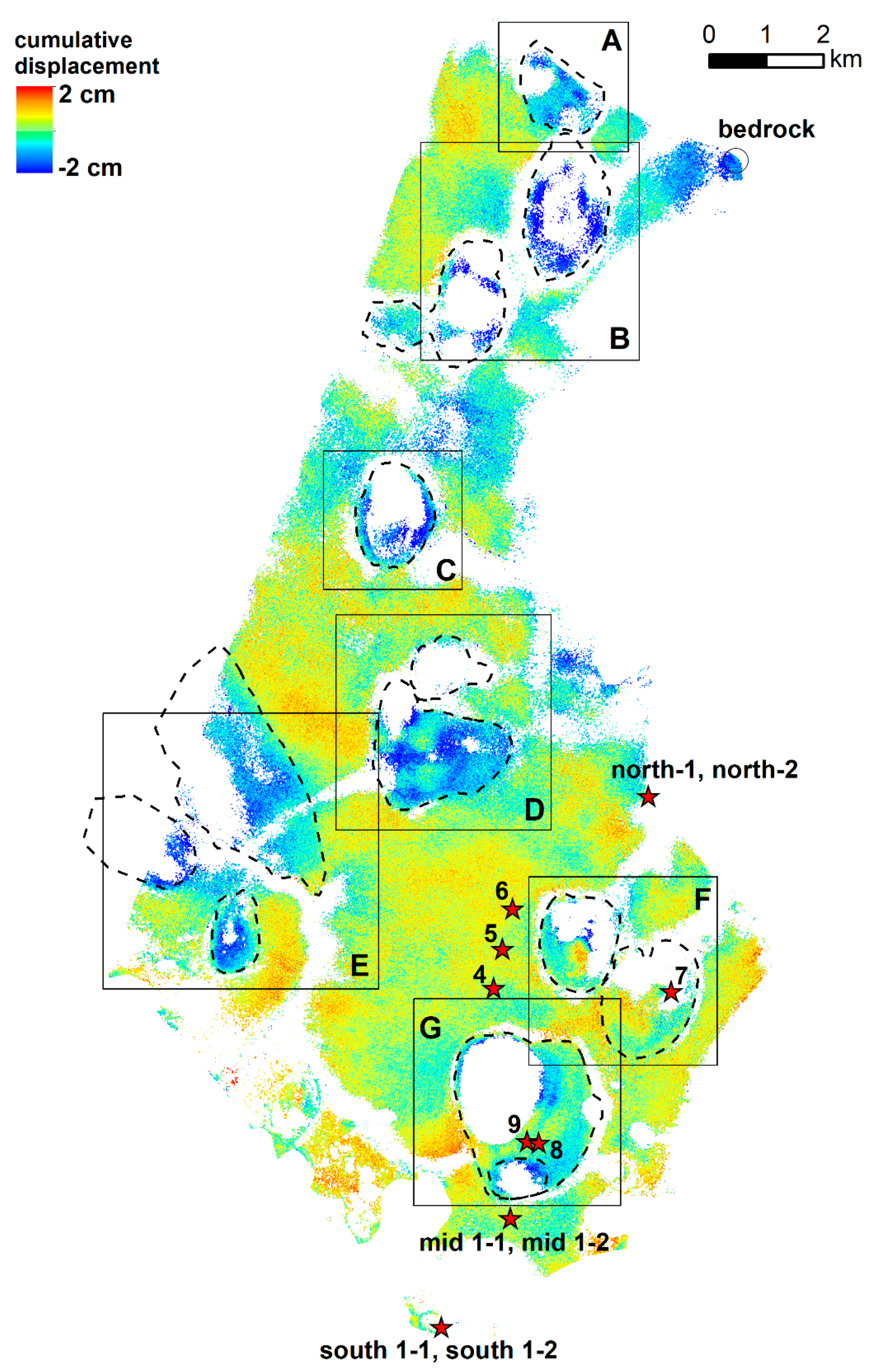
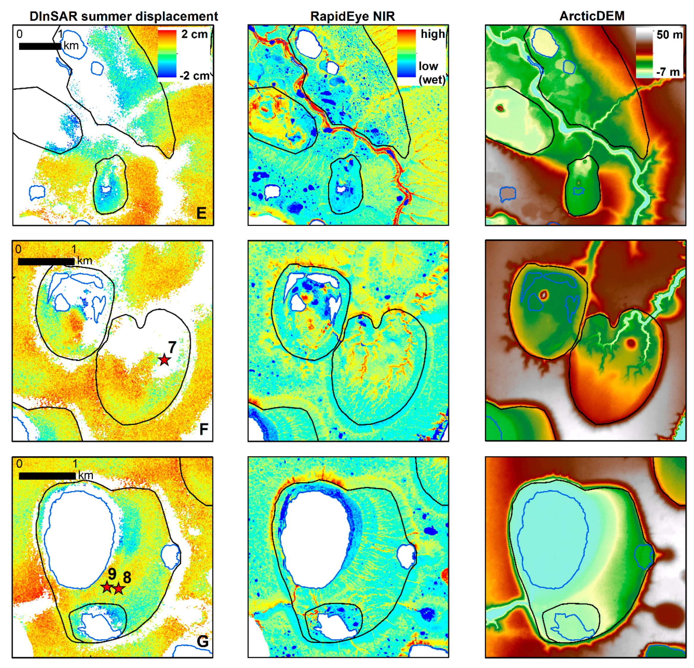
4.1.3. Spatial Variability

The spatial variability of subsidence on different scales was investigated using sets of stations with different spacing between them (see Data and Methods). Figure 5a shows the variability of seasonal subsidence measured at each of the station sets (7, 8, 9 with 0.5–1 m spacing) and along the transect (25 m spacing) in late August 2014 relative to April 2014. Station sets 7 and 9 demonstrated the most consistent subsidence magnitude with average values of 7.3 ± 0.9 cm and 5.3 ± 1.2 cm, respectively. Station set 8, however, showed a wider range of subsidence values, with an average of 4.9 ± 2.4 cm. The transect showed a range of subsidence values, characterized by an average value of 2.9 ± 1.3 cm.

In addition, measurements from metal stations within the sets showed subsidence values similar to those from fiberglass stations. Although fiberglass stations are characterized by a much lower thermal conductivity and are thinner in diameter than steel pipes, there appears to be no difference between metal and fiberglass materials in terms of performance for displacement measurements.

Additionally, two pairs of metal stations installed in 2013 had an approximate spacing of 5 m within each pair. Local topography and surface conditions were distinctly different for each station within a pair. Two stations were located on a relatively dry surface with little vegetation (mid-1 and south-1), whereas two other stations were located in wet local depressions with thick and wet moss layer and grasses (mid-2 and south-2). Figure 5b shows relative seasonal displacement for these four stations in 2013 and 2014. In late August 2013, stations located on dry surfaces showed subsidence of 2.3 and 2.4 cm, whereas stations located in wet depressions showed almost no displacement. In mid-August 2014, all four stations showed a pronounced subsidence. However, one of the dry sites showed approximately 3 cm more subsidence than the wet sites.

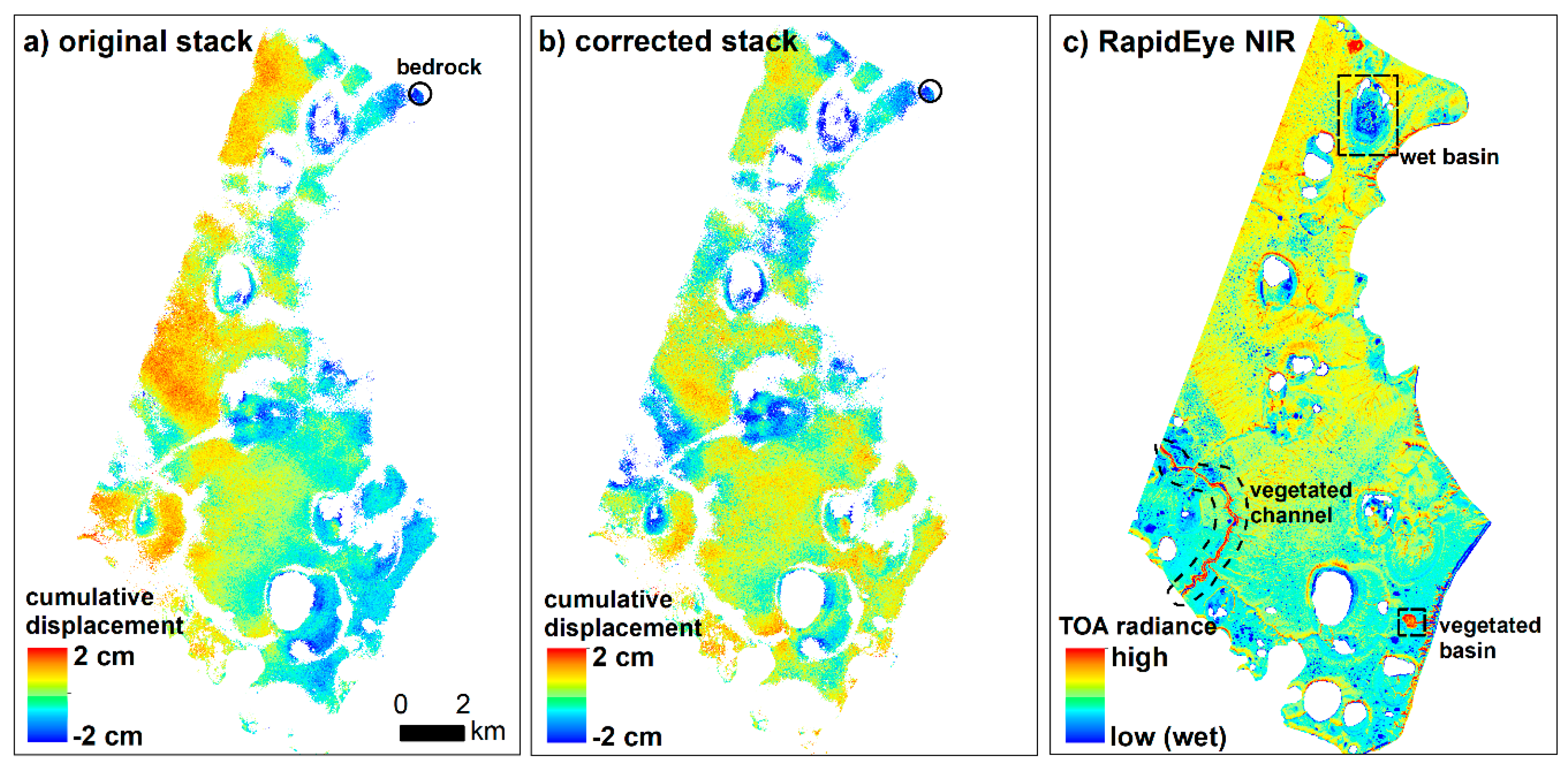
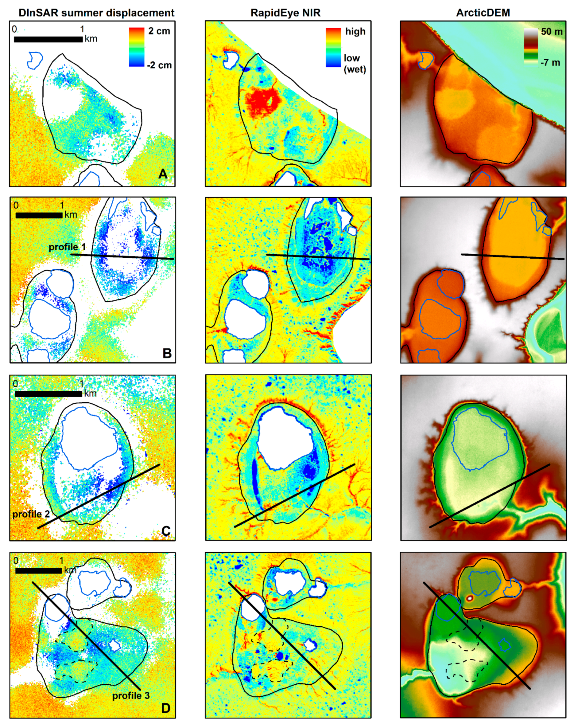
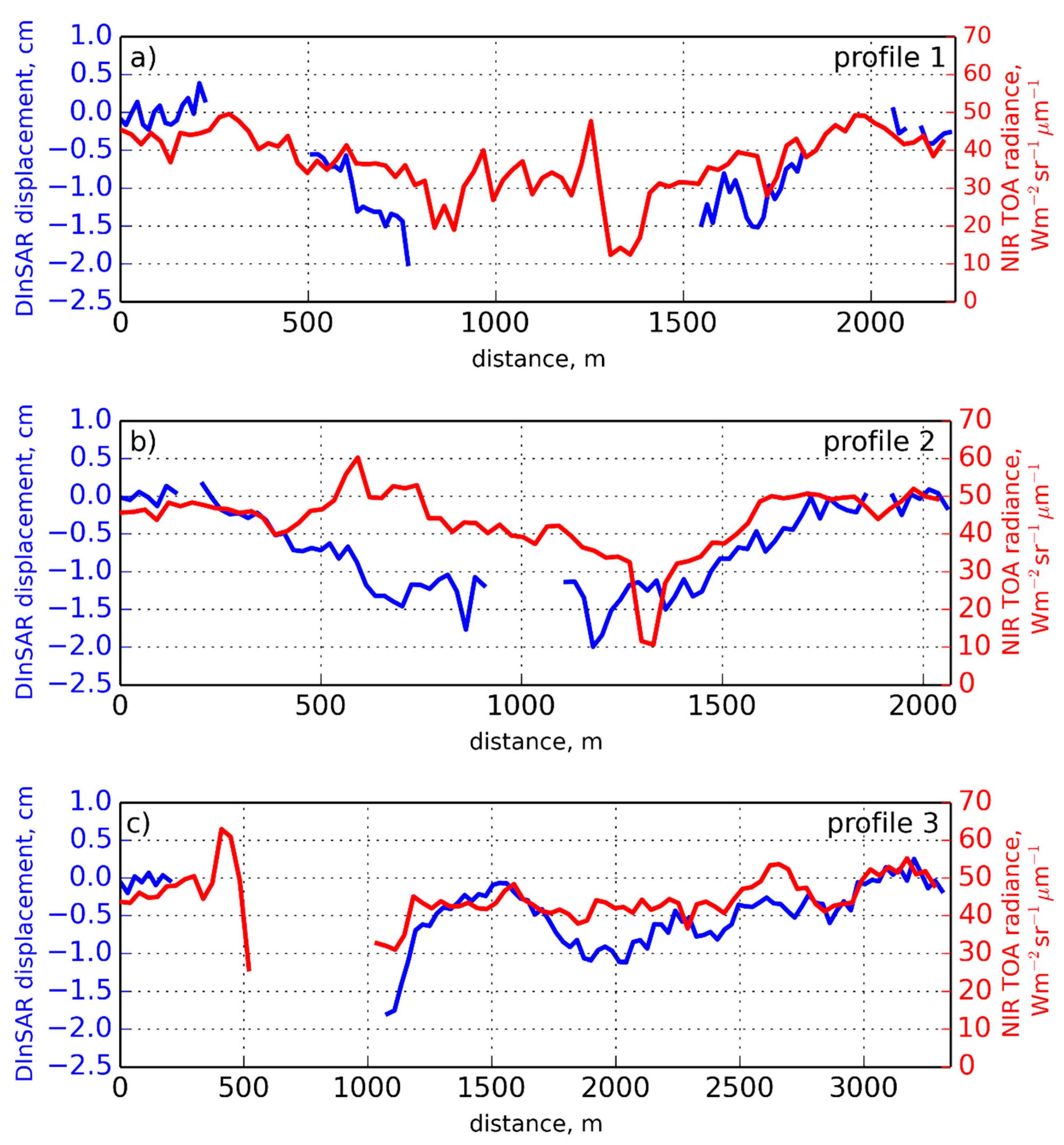
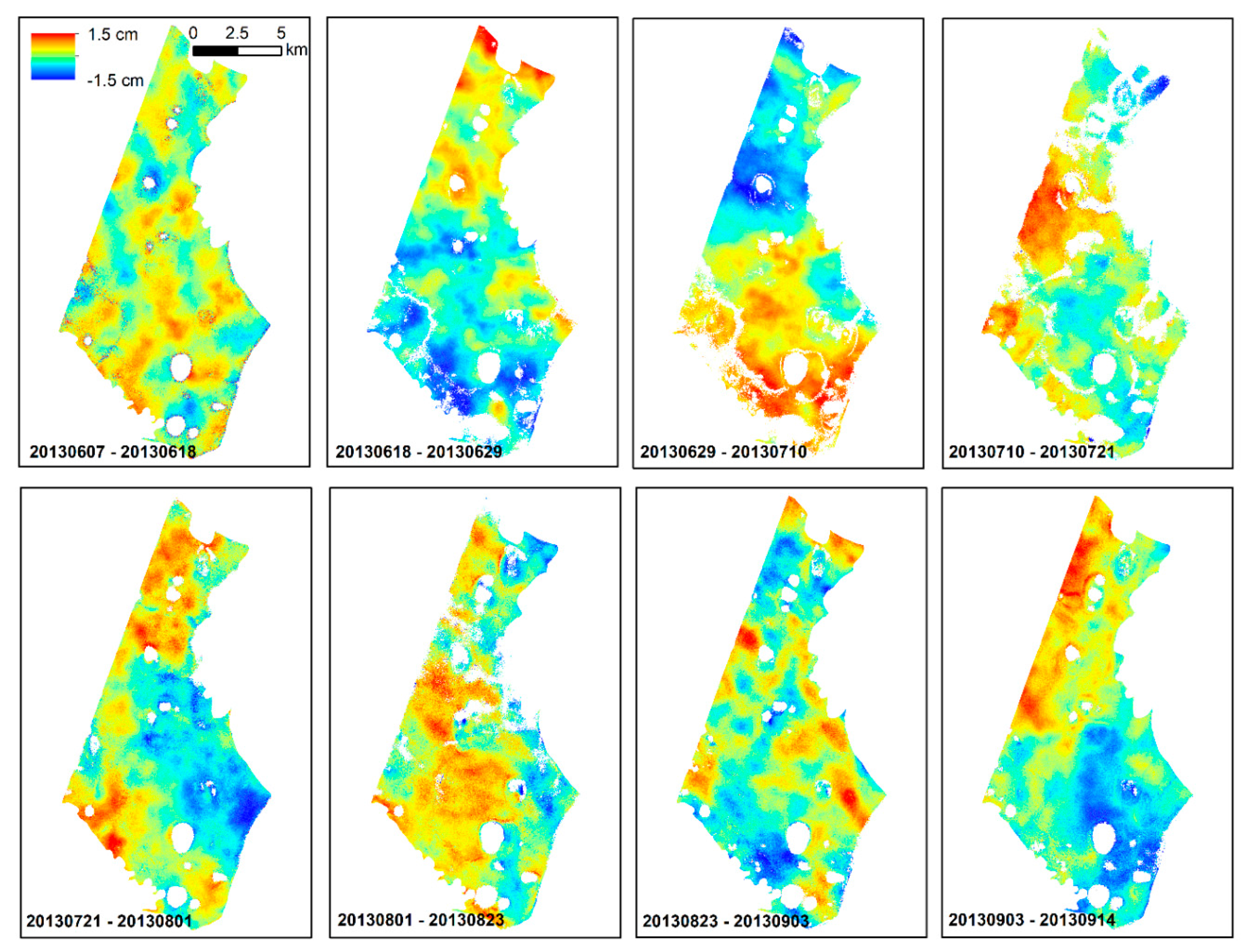
4.2. DInSAR

After removing the ramp from the cumulative displacement map, most of the island showed an uplift with a median value of 0.44 cm and a standard deviation of 0.41 cm (Figure 6). We relate this to possible errors due to the choice of reference point and residual atmospheric signal rather than to real ground motion which is expected to be downward during the summer.

We checked to determine whether the relative difference in the in situ measured subsidence is captured by the relative difference in the DInSAR displacement values. A total of 12 metal stations was installed in April 2013; only eight of these stations were measured at the end of August 2013 due to logistic reasons, and of these eight measured stations, only six were covered by valid DInSAR pixels. Of these six stations, two were located within one DInSAR pixel. We compared these six in situ measurements with five DInSAR values, taking each of the two in situ measurements within one pixel separately (Figure 7).

For both sets of in situ measurements, the agreement with DInSAR displacement values was moderate, with the correlation coefficient of 0.5 and 0.42, respectively. We acknowledge, however, that statistical analysis is not really possible with only five measurements. We also note that the DInSAR displacement map spanned a time period until the middle of September, whereas in situ measurements were made at the end of August, potentially missing some signal.

Whereas the DInSAR cumulative displacement map generally did not show the expected subsidence, distinct downward motions of up to 2 cm were present in most of the thermokarst basins (Figure 6). We took a closer look at some selected thermokarst basins (Figure 8). Different basins showed different displacement behavior. Thus, the basins in A, B, C, D, and E mostly subsided, whereas most parts of the basins in F and G showed uplift or relative stability (Figure 8 column 1). The strongest subsidence occurred in the basins in B and C and in some parts of the basin in D. We compared the DInSAR displacement patterns with the spatial patterns of the RapidEye NIR band (Figure 8 column 2).

The low NIR TOA values in the subsiding basins (Figure 8A–E) suggest that these basins consist of parts, which are considerably wetter compared to the surrounding upland. The basins in F and G do not appear wetter than the upland, so this lack of wetness contrast likely also results in the lack of contrast on the DInSAR map. The large basin in D showed a peculiar displacement pattern; two marked areas of slight uplift/stability correspond to the relatively dry parts of the basin, whereas areas that exhibited subsidence roughly correspond to the relatively wetter part of the basin. The small central part of the left basin in F, which showed relatively strong subsidence, also corresponds to the wet part of the basin indicated by low NIR TOA. The same is true for the small basin located in the southern part of a large basin in G and for the area to the right of a big lake in G.

We also analyzed three profiles across three selected basins (Figure 8B–D) to follow the spatial variations of the subsidence and relative wetness (Figure 9). Each point on a profile is the average of 5 pixels across the profile (25 m) and 3 to 4 pixels along the profile (15–20 m). Because we are not certain of displacement values on the upland, we manually shifted them to approximately zero level and consider the subsidence within the basins relative to the upland. Profile 1 shows a gradual increase of subsidence simultaneous with an increase of wetness in the western part of the profile, and a gradual decrease of subsidence simultaneous with a decrease of wetness in the eastern part of the profile, with a maximum subsidence of approximately 1.7 cm. The pattern of subsidence along profile 2 is similar and reach 2 cm maximum. Variations of the wetness along profile 2 correspond to the variations of subsidence in the eastern part of the profile. Profile 3 shows the maximum subsidence of approximately 1.7 cm at a distance of approximately 1100 m from the beginning of the profile, which then gradually decreases to roughly zero level, then increases further up to 1.5 cm and then slightly decreases again. The wetness along profile 3 corresponds to the subsidence variations at some parts of the profile.

5. Discussion

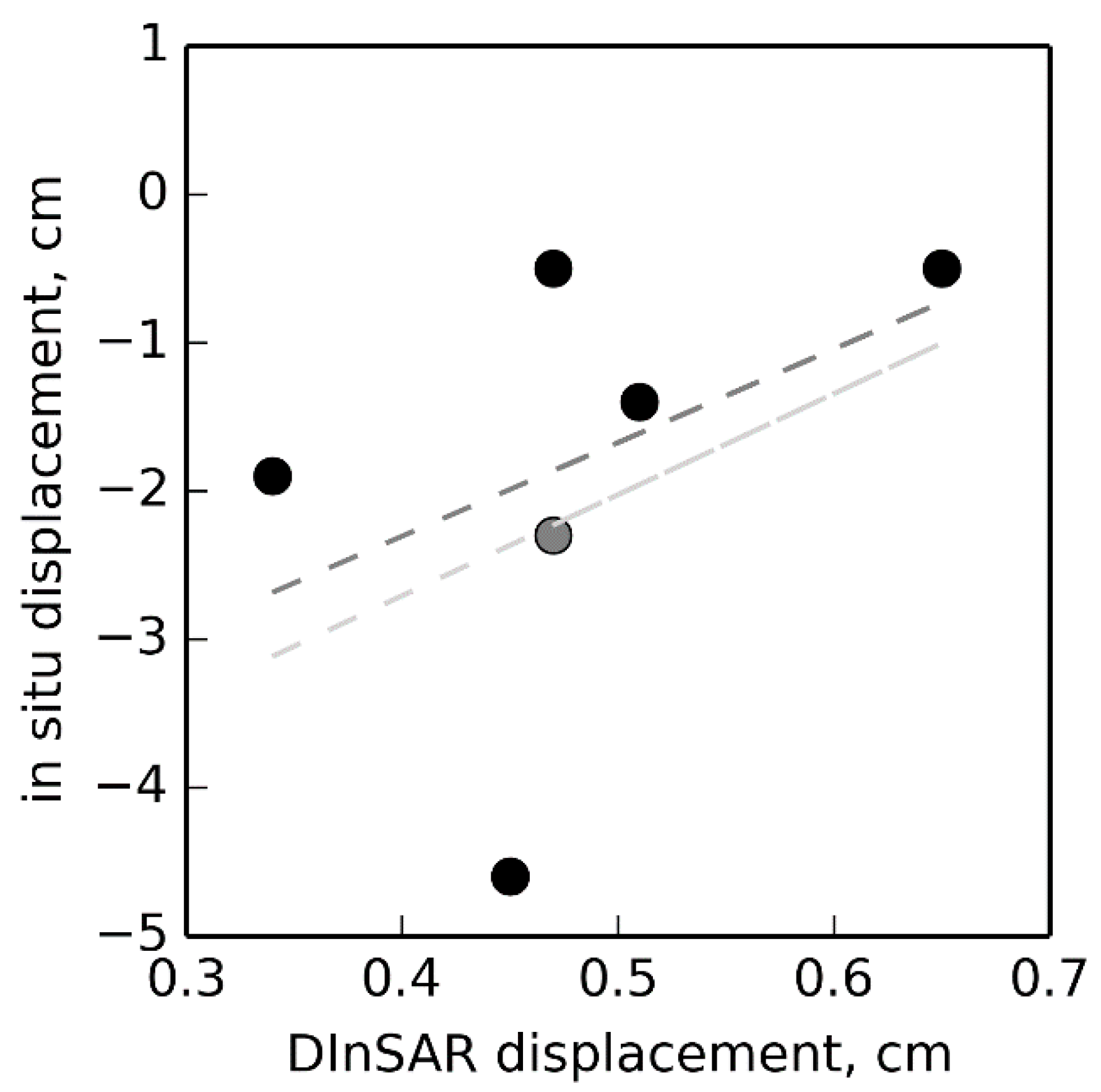
5.1. Validity of In Situ Measurements

We have shown that, for our reference rods, holding force prevailed over heaving force. In our calculations we had to follow some simplifications and assumptions, e.g., when referring to the building code for adfreezing strength and shear resistance values for different soil texture and moisture as well as the material of the rods. Therefore, we admit the possibility that the rods could experience heaving during the freezing season. This, however, does not affect our measurements of seasonal subsidence in 2013 for the stations installed in April 2013 and seasonal subsidence in 2014 for the stations installed in April 2014. Another confirmation that our subsidence observations are not purely due to the heaving of the rods is the observed ground uplift during some seasons (i.e., decreasing distance between the top of the rod and the ground surface). Such an uplift would mean that the rods would sink into the permafrost, which is not possible.

5.2. Temporal Variability of Ground Movements

Two summer seasons (2013 and 2014) clearly demonstrated different seasonal subsidence magnitudes with median values of 1.6 cm in 2013 and 4.7 cm in 2014. This difference can logically be attributed to the difference in climatic conditions of these two summer seasons. Based on air temperature measurements from a meteorological station nearby (http://rp5.ru/Weather_archive_on_Stolb_Island), we calculated the square root of the thawing degree days (TDD) index for the last decade (Figure 10). This index is the sum of daily air temperatures of each day of a year with temperature >0 °C. Additionally, we considered active layer depths measured at Bykovsky Peninsula within the Circumpolar Active Layer Monitoring (CALM) program (71°47.13′N, 129°25.15′E; site code R29A). This measurement site is located on yedoma deposits which have the same origin as yedoma deposits found in our study area. Clearly, 2013 was one of the two coldest years of the last decade, which is well reflected by the low TDD and shallow active layer depths. These exceptionally cold conditions explain less seasonal subsidence in 2013 compared to 2014. These different summer preconditions also led to a difference in observed multiyear displacement: April 2014 (after the cold summer of 2013) demonstrated both uplift and subsidence relative to the April 2013 reference, whereas April 2015 (after the warm summer of 2014) showed clear subsidence relative to both the April 2013 and April 2014 references. Considering that only two years of the past decade were relatively cold (2009 and 2013), it is likely that the net subsidence accumulates from year to year because there have been insufficient cold years to reverse or significantly slow down subsidence. This is also confirmed by a substantial subsidence (9.3 ± 5.7 cm) observed for all reference stations between 2013 and 2017.

5.3. Connection to Other Studies

Studies from Alaska over longer time periods support our observations. Streletskiy et al. [8] continued repeat DGPS measurements from Shiklomanov et al. [5] and report a net average subsidence of up to 15 cm for the period from 2003 to 2015 in Utquigvik, Alaska (known at that time as Barrow). They associate the observed net subsidence with increasing air temperatures and consequent thawing of the ice-rich layer at the permafrost table. Liu and Larson [36] use a novel method based on reflected GPS signal and observe mean seasonal thaw subsidence of 3.3 ± 0.2 cm and an overall decadal subsidence rate of 0.26 ± 0.02 cm per year from 2004–2015. In the Siberian Arctic, Günther et al. [14] used the difference between DEMs from 1951 and 2013 to estimate the long-term ground subsidence on Muostakh Island (southern Laptev Sea). The Ice Complex deposits there have the same origin as the Ice Complex deposits in our study area. They found an average net subsidence of 3.6 ± 1.8 m over 62 years, providing strong evidence of long-term ground ice melt.

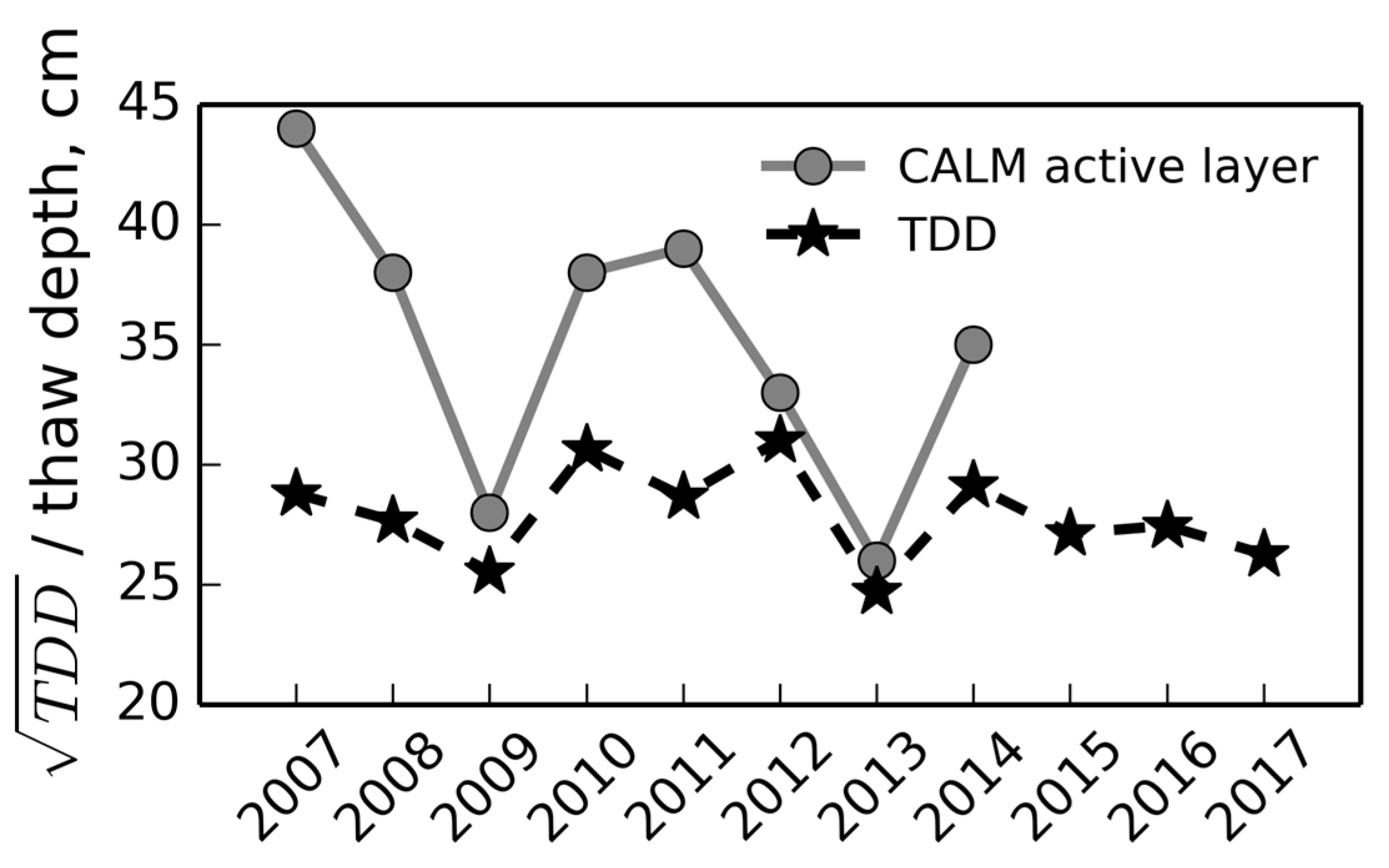
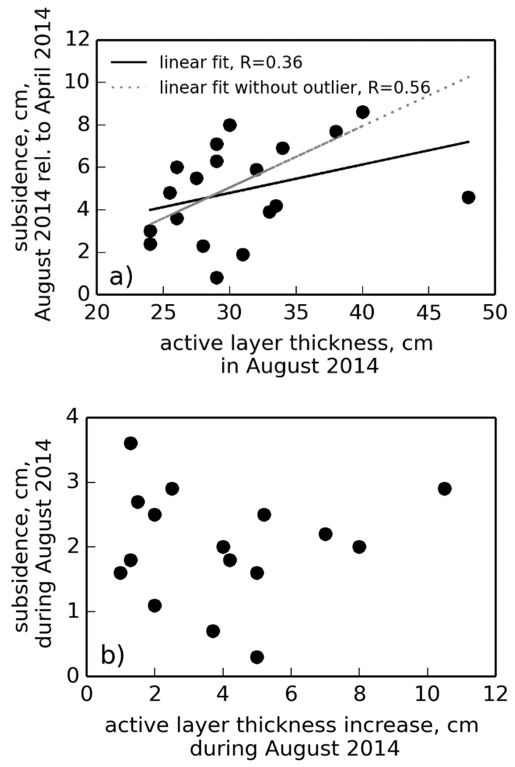
5.4. Relation between Subsidence and Active Layer Depth

We quantified the relationship between seasonal subsidence and active layer depth, measured exactly at the reference rods in the beginning and at the end of August 2014. Figure 11a shows the relation between active layer depths measured at the end of August 2014 and the seasonal subsidence relative to the reference winter observations. Whereas the full set of observations does not show a substantial correlation (0.36), removal of one outlier results in an improvement of correlation up to 0.56. Figure 11b shows no relation between the increase of active layer depth and increase of subsidence during August 2014.

In comparison, Günther et al. [14] observed a counterintuitive inverse relation between the multi-decadal subsidence and active layer depth on Muostakh Island. They explain this by the fact that a shallow active layer was associated with near-surface ground ice, whereas a deep active layer was generally found on well-drained slopes, which are less prone to the subsidence. Siewert et al. [37] also found a deeper active layer on the slopes of thermokarst basins compared to the undegraded yedoma upland on Kurungnakh Island.Our in situ observations are much sparser, however, than observations in those studies and do not cover a wide range of landscape forms and active layer depths.

Conversely, Liu et al. [38] model the active layer thickness using the ERS-1/2 DInSAR observations of seasonal subsidence using the direct relation between these variables. They assume that melt of ice in soil pores and related volumetric change is the main mechanism of seasonal subsidence. We calculate the potential subsidence due to the volumetric change between ice and water within the active layer in our study following the simplistic approach by [38]

$$d=ALT·VWC·0.1$$

(4)

where $d$ is potential subsidence due to melting of pore ice, $ALT$ is the active layer thickness, $VWC$ is volumetric water content, and 0.1 represents the volumetric difference between ice and water. We collected $VWC$ measurements using time-domain reflectometry in July 2013 at a number of vertical profiles in the vicinity of reference rods. We calculated the potential subsidence for each ground layer where we had $VWC$ measurements and summed it up for each profile. Here, we provide the comparison between the potential subsidence and the measured subsidence at 10 stations at the time of $VWC$ measurements (

Table 2. Potential subsidence due to volumetric change in soil pores and actual subsidence measured in July 2013. Negative values represent uplift, which can be explained by either growing vegetation or uncertainties inherent in the manual measurements.

Station	Potential Subsidence, cm	Measured Subsidence, cm
south-1	0.88	1.4
south-2	0.51	−0.4
mid-1	0.26	−0.1
mid-2	0.44	0.2
north-1	0.6	0.1
north-2	0.63	1.4
4	0.58	1.5
7	0.73	4.3
8	0.24	−0.4
9	0.44	0.5

).

The potential and measured subsidence are generally correlated with a correlation coefficient of 0.65, meaning that this simplistic approach can provide a meaningful estimation of the subsidence. However, other processes besides volumetric change in soil pores, likely contribute to the net subsidence as well. We also note that these calculations are made for the measurements from July, when the active layer and subsidence did not reach their yearly maximum.

5.5. Spatial Variability of Subsidence

In our study, subsidence measurements also demonstrated high variability on different spatial scales. In 2013, seasonal subsidence varied from 0 to 4.6 cm for sites separated by a few kilometers. Smaller site separation distances on the order of a few meters showed that the subsidence likely depended on the local microtopography and surface wetness (Figure 5b). More specifically, two dry sites showed greater subsidence when compared to two wet sites, which featured almost no displacement. This observation might be explained by a difference in the surface energy balance, i.e., evapotranspiration, sensible heat flux, and ground heat flux [39]. However, the difference between wet and dry sites was only partly sustained in summer 2014, when both wet sites experienced the same amount of subsidence as one of the dry sites, while the other dry site subsided twice as much. It is possible that higher air temperatures in summer 2014 allowed for deeper thawing, thus dominating over surface wetness effects. It is also likely that the local ground ice variations are responsible for the spatially varying subsidence.

The installation of a number of additional stations in 2014 allowed us to detect spatial variability of subsidence on a small horizontal scale. Within a 0.5–1 m spacing, seasonal subsidence in 2014 varied by as little as 2.3 cm (station set 7) and by as much as 5.6 cm (station set 8). Shiklomanov et al. [5] investigated the scale of maximum subsidence variability in Alaska. They observed the maximum variability at separation distances of 30 m and greater on the Alaskan coastal plain, which they attributed to differences between landscape elements (thermokarst basins and upland tundra). On the contrary, we did not find any difference in subsidence magnitudes measured in situ in the thermokarst basins (4.3 ± 2 cm, 31 measurements) and on the yedoma upland (4.6 ± 1.5 cm, 9 measurements). Similar to our study and unlike the Alaskan coastal plain, the northern foothills of the Brooks Range show the maximum variability at separation distances of 1–3 m; this variability is governed by vegetation cover and microtopography, represented by multiple frost boils [5]. Overduin and Kane [40] measured ground displacement in situ specifically at frost boils in the Brooks Range between 2001 and 2005. They found higher net subsidence rates at frost boil centers (5–7.5 cm per year) compared to the surrounding tundra (2–5 cm per year) over four years of measurements and explained this difference by the absence of an insulating organic layer over the boils. At our study site, Siewert et al. [37] performed field observations at 50 vertical profiles in summer 2013 and observed a high heterogeneity of the sub-ground properties on a meter scale due to a widespread occurrence of cryoturbation. This observation robustly supports our field evidence of highly variable subsidence.

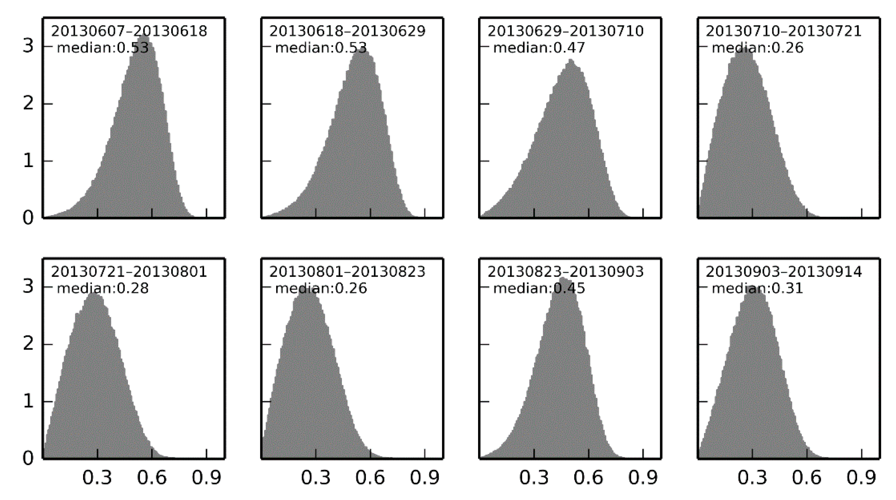
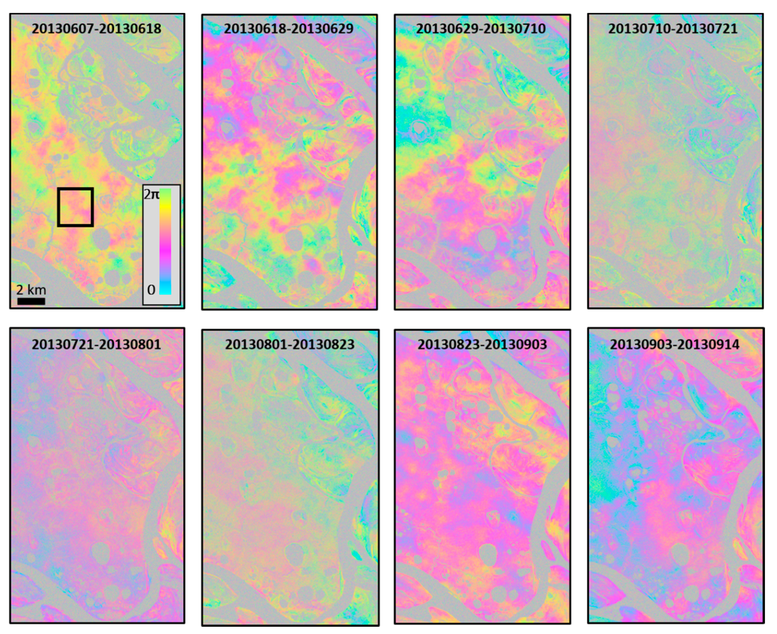
5.6. DInSAR: Results, Errors, Validation, and Prospectives

The cumulative displacement map obtained from a stack of TSX DInSAR interferograms for summer 2013 did not show a general and widespread subsidence pattern. To interpret the long-wavelength negative phase changes as uplift is not plausible with the natural processes. We assume that with a few interferograms we could not reduce the atmospheric effect to a low level required for a stable estimation of long-wavelength surface displacement signal. Also, the deramping could possibly have led to some undesirable effects. We further acknowledge possible errors related to the choice of the reference point for the phase unwrapping, especially considering that the reference point is remote from our area of interest and only weakly connected to the rest of the map over a small and noisy area of valid pixels (Figure 6). Unfortunately, we have no information about more stable bedrock locations and therefore better suited reference points to improve the displacement stack.

Therefore, we look at smaller scales with varying local references for the surface displacement signal, i.e., (i) relative difference among the in situ measurements versus DInSAR displacements and (ii) subsidence in the thermokarst basins relative to the island’s upland.

Comparing the surface displacements measured in situ and by DInSAR, we observed a moderate correlation between in situ observations and the colocated averaged DInSAR values. However, even this moderate correlation is surprising, assuming the arbitrary position of a single in situ measurement within the pixel area. In our in situ measurements (although made in 2014 versus the DInSAR in 2013), we observed high spatial variability of subsidence (up to 6 cm) even on a sub-meter scale. Therefore, it seems to be impossible to determine a representative validation measurement for a pixel without performing subpixel statistics. For that, much denser in situ observations should be done in future. High-resolution unmanned aerial vehicle (UAV) or terrestrial laser scanning surveys could also be used to resolve the subpixel variability of permafrost freeze/thaw ground motion. A number of previous studies exploit DInSAR to quantify thaw subsidence in permafrost landscapes (e.g., [12,13,15,16,18,41,42]). Although these studies report the successful retrieval of seasonal and multi-year subsidence, most of them lack verification with in situ measurements. Short et al. [12] used two thaw-tubes to validate RADARSAT-2 DInSAR results in the Iqaluit Airport, Baffin Island, Canada. Wang et al. [13] also compared ALOS-PALSAR interferometric subsidence over permafrost mounds in northern Quebec, Canada, with two thaw-tube measurements. In both studies, DInSAR captures the spatial variability in subsidence qualitatively but not quantitatively.

The subpixel variability not only poses a question for a validation strategy but can also be a source of problems for DInSAR itself. Heterogeneous displacement within a pixel can lead, first, to phase decorrelation, and, second, to systematic errors in DInSAR estimations. Zwieback et al. [20] used a statistical phase closure test to show that various environmental processes can systematically influence the DInSAR phase. They used the same TSX dataset as in our study and show that significant phase closure errors at our study area (yedoma upland) could amount to as much as 10% during summer 2013. However, the real impact on the estimated displacement may be substantially larger than the phase closure error, especially in the case when the examined ground displacements are on the same order of magnitude as the phase closure. They propose that heterogeneous surface movements and soil moisture changes are the main processes responsible for the systematic errors.

Studying the relative changes of DInSAR-measured displacements along smaller distances, we observed a particularly strong signal from upland to thermokarst basins, i.e., subsidence by up to 2 cm. This signal cannot be attributed to the atmospheric effects due to its very distinct extent (Figure 6). This signal corresponds well with findings in the study of Liu et al. [41]. Using ALOS-PALSAR interferometry they show that among 18 studied drained thermokarst lake basins in Prudhoe Bay, Alaska, five basins exhibited seasonal subsidence much greater than that of the surrounding tundra upland (four basins exceeded 4 cm and one basin exceeded 12 cm). Their profile of subsidence across a basin is very similar to two profiles in our study (Figure 9a,b), with more subsidence in the center of the basin and less subsidence at the margins. They interpret this spatial variability using ground penetrating radar (GPR) data and suggest that the thawing of especially ice-rich fine-grained lake sediments, which likely contain segregated ice, is responsible for the observed strong subsidence. Similarly, Haghshenas Haghighi et al. [43] show more subsidence in some of the thermokarst basins compared to tundra uplands in Utquigvik, Alaska (known at that time as Barrow) using TSX DInSAR analysis.

A remarkable observation of our study is that the spatial distributions of the subsidence and the surface wetness in the basins were in high agreement (Figure 8 and Figure 9). Drier parts of the basins were clearly separated from wetter parts that showed a prominent subsidence. This might be explained by the higher ground ice content of the wet parts and also by a higher ground heat flux in the wet part due to higher thermal conductivity. Our in situ measurements did not reveal more subsidence in the thermokarst basins compared to the surrounding upland. However, our in situ measurements in the basins are located either in the decorrelated part of the DInSAR map (station 7) or in a dry part of the basin (stations 8 and 9), which did not exhibit DInSAR-subsidence (Figure 8F,G). A greater subsidence in the wetter parts of the basins seems contradictory to our in situ observations on the upland with two pairs of reference rods (Figure 5b). In these observations, drier sites subsided more than wetter sites, and we explained this with the different amount of energy required for the evaporation at the dry and wet sites (e.g., [44]). However, the scales of the two phenomena are not comparable: subsiding dry sites from the field observations rather represent the microtopographical features (e.g., hummocks and inter-hummock spaces), whereas the subsiding wet basins from the DInSAR analysis represent the landscape unit with an areal size of hundreds of meters. Thus, the local wet sites on the upland can be considered as part of the generally dry landscape, whereas wet thermokarst basins are represented by saturated polygonal tundra with patches of open water.

From the DInSAR methodological point of view, such spatial agreement between surface wetness and subsidence proves that the atmospheric effect has no major influence on the DInSAR cumulative displacement map, at least on the scale of roughly the size of a thermokarst basin. It is likely that the choice of the reference point as well as filtering or unwrapping artifacts had the strongest influence on the result in our study and can explain the apparent slight uplift over the island’s upland. Another observation is that the areas of greater subsidence and higher wetness in our study were found close to the areas of coherence loss; if the area becomes too wet, the coherence drops dramatically, and interferometric analysis of the area becomes impossible. A subtle border of the critical wetness seems to rule the feasibility of DInSAR analysis for TSX in the thermokarst basins environment. Another consideration is that the coherent DInSAR signal from the wet basins can possibly be dielectrically affected by ground wetness, and the observed subsidence is partly interfered with a steady drying of the ground, i.e., after snowmelt (e.g., [19]). However, this scenario would mean (i) the presence of a steady drying process over the summer ignoring the influence of precipitation events and (ii) that the wet parts of the basins dry faster than the dry parts, which seems to be unlikely.

A persistent isotropic thaw subsidence was reported from different Arctic permafrost areas (e.g., [5,8,14,36]) and was related to increasing summer air temperatures. According to the modelled prognosis, the warming trend will persist in the future, meaning that monitoring of thaw subsidence in permafrost areas will be a high priority. Satellite geodetic methods offer DInSAR, multitemporal DEMs differencing, and reflected GPS signals from a network of continuously operating GPS receivers. Our findings show the practical unfeasibility of X-band DInSAR for multi-year subsidence monitoring due to a quick coherence loss, which confirms previous studies (e.g., [13,18]). C-band and L-band sensors, such as currently operating Sentinel-1 and ALOS-2 PALSAR-2 can maintain high coherence on multi-year time spans and, therefore, be used in monitoring of long-term subsidence. The method of DEMs differencing is not affected by inherent DInSAR problems and seems to be promising for the detection of subsidence with magnitudes exceeding the DEMs accuracy. Recently issued global TanDEM-X DEM provides new opportunities for long-term subsidence monitoring in permafrost areas. The application of reflected GPS signals for subsidence monitoring has proved its feasibility [36], but provides observations for only a limited number of points where the GPS receivers are installed.

6. Conclusions

This study contributes to the developing method of DInSAR estimation of ground displacements related to thawing and freezing processes in permafrost environments. For the first time, numerous field measurements accompanied a permafrost DInSAR study in the Siberian Arctic. These measurements, performed on a yedoma island in the Lena River Delta from 2013–2017, detected pronounced seasonal and multi-year net subsidence. The temporal variability in the magnitude of subsidence was related to distinct interannual air temperature variations and subsequent variations in thaw penetration into the ground. An important observation was the high spatial inhomogeneity (sub-meter scale) of subsidence.

We tested repeat-pass StripMap TSX data for their applicability in detecting the in situ observed subsidence. A sequence of 11-day partly coherent interferograms was available for summer 2013. We show the interferometric processing steps and intermediate results to demonstrate the general limitations of X-band DInSAR for permafrost subsidence monitoring. Low coherence in combination with atmospheric effects as well as remoteness of a reference ground point were severe obstacles for the retrieval of a wide-area seasonal thaw subsidence map. The multi-temporal interferometry techniques, which combine interferograms with varying time spans and efficiently reduce the atmospheric signal, could not be implemented here due to the rapid drop of coherence starting in many cases already at the 22-day time span. In agreement with previous studies, we suggest that the greater radar wavelengths such as C-band and L-band can maintain high coherence on longer time spans and, therefore, can provide more opportunities for the DInSAR estimations of the ground movements in permafrost environments, but at the same time can be more influenced by soil moisture effects. By showing the sub-pixel variability of the subsidence we identified a problem for the validation of DInSAR ground movement estimations. A detailed scheme for the validation needs to be developed and implemented in future studies.

Although we could not observe the seasonal thaw subsidence over most of the island’s upland with the TSX DInSAR analysis, many of the thermokarst basins, which in total occupy about 40% of the island’s area, showed a distinct subsidence signal of up to 2 cm relative to the upland, which agrees with two previous studies. Moreover, the magnitude of subsidence in the basins was in high spatial agreement with the relative surface wetness, estimated from the NIR band of a high resolution optical image RapidEye. The dielectrical influence of the surface wetness on the DInSAR phase cannot, however, be completely excluded and might influence the DInSAR subsidence estimations. Future field observations of subsidence together with detailed analysis of the sub-ground and surface properties, i.e., ground ice content and surface wetness, in wet and dry parts of thermokarst basins can provide highly valuable insights for the development of DInSAR methodology in permafrost environments.

References

- Zhang, T.; Barry, R.G.; Knowldes, K.; Heginbottom, J.A.; Brown, J. Statistics and Characteristics of Permafrost and Ground-Ice Distribution in the Northern Hemisphere. Polar Geogr. 1999, 23, 132–154. [Google Scholar] [CrossRef]
- Melnikov, P.I. Vliyanie podzemnykh vod na glubokoe okhlazhdenie verkhnej zony zemnoj kory (Influence of ground waters on the deep cooling of upper Earth crust). In Merzlotno-Gidrogeologicheskie i Gidrogeotermicheskie Issledovaniya na Vostoke SSSR (Cryo-Hydrogeological and Hydrogeothermal Investigations in the East of USSR); Nauka: Moscow, USSR, 1967; pp. 24–29. (In Russian) [Google Scholar]
- French, H.M. The Periglacial Environment, 3rd ed.; John Wiley & Sons, Ltd.: West Sussex, UK, 2007. [Google Scholar]
- Langer, M.; Westermann, S.; Heikenfeld, M.; Dorn, W.; Boike, J. Satellite-based modeling of permafrost temperatures in a tundra lowland landscape. Remote Sens. Environ. 2013, 135, 12–24. [Google Scholar] [CrossRef]
- Shiklomanov, N.I.; Streletskiy, D.A.; Little, J.D.; Nelson, F.E. Isotropic thaw subsidence in undisturbed permafrost landscapes. Geophys. Res. Lett. 2013, 40, 6356–6361. [Google Scholar] [CrossRef]
- Little, J.D.; Sandall, H.; Walegur, M.T.; Nelson, F.E. Application of differential global positioning systems to monitor frost heave and thaw settlement in tundra environments. Permafr. Periglac. Proc. 2003, 14, 349–357. [Google Scholar] [CrossRef]
- Beck, I.; Ludwig, R.; Bernier, M.; Strozzi, T.; Boike, J. Vertical movements of frost mounds in subarctic permafrost regions analyzed using geodetic survey and satellite interferometry. Earth Surf. Dyn. 2015, 3, 409–421. [Google Scholar] [CrossRef]
- Streletskiy, D.A.; Shiklomanov, N.I.; Little, J.D.; Nelson, F.E.; Brown, J.; Nyland, K.E.; Klene, A.E. Thaw subsidence in undisturbed tundra landscapes, Barrow, Alaska, 1962–2015. Permafr. Periglac. Proc. 2016, 28, 566–572. [Google Scholar] [CrossRef]
- Harris, C.; Luetschg, M.; Davies, M.C.; Smith, F.; Christiansen, H.H.; Isaksen, K. Field instrumentation for real-time monitoring of periglacial solifluction. Permafr. Periglac. Proc. 2007, 18, 105–114. [Google Scholar] [CrossRef]
- Akagawa, S.; Huang, S.L.; Kanie, S.; Fukuda, M. Movement due to heave and thaw settlement of a full-scale test chilled gas pipeline constructed in Fairbanks Alaska. In Proceedings of the OTC Arctic Technology Conference, Houston, TX, USA, 3–5 December 2012; Offshore Technology Conference: Houston, TX, USA, 2012. [Google Scholar]
- Nixon, M.; Tarnocai, C.; Kutny, L. Long-term active layer monitoring: Mackenzie Valley, northwest Canada. In Proceedings of the 8th International Conference on Permafrost, Zurich, Switzerland, 21–25 July 2003; pp. 821–826. [Google Scholar]
- Short, N.; LeBlanc, A.-M.; Sladen, W.; Oldenborger, G.; Mathon-Dufour, V.; Brisco, B. RADARSAT-2 D-InSAR for ground displacement in permafrost terrain, validation from Iqaluit Airport, Baffin Island, Canada. Remote Sens. Environ. 2014, 141, 40–51. [Google Scholar] [CrossRef]
- Wang, L.; Marzahn, P.; Bernier, M.; Jacome, A.; Poulin, J.; Ludwig, R. Comparison of TerraSAR-X and ALOS PALSAR Differential Interferometry With Multisource DEMs for Monitoring Ground Displacement in a Discontinuous Permafrost Region. IEEE J. Sel. Top. Appl. Earth Obs. Remote Sens. 2017, 10, 4074–4093. [Google Scholar] [CrossRef]
- Günther, F.; Overduin, P.P.; Yakshina, I.A.; Opel, T.; Baranskaya, A.V.; Grigoriev, M.N. Observing Muostakh disappear: Permafrost thaw subsidence and erosion of a ground-ice-rich island in response to arctic summer warming and sea ice reduction. Cryosphere 2015, 9, 151–178. [Google Scholar] [CrossRef]
- Rykhus, R.P.; Lu, Z. InSAR detects possible thaw settlement in the Alaskan Arctic Coastal Plain. Can. J. Remote Sens. 2008, 34, 100–112. [Google Scholar] [CrossRef]
- Liu, L.; Zhang, T.; Wahr, J. InSAR measurements of surface deformation over permafrost on the North Slope of Alaska. J. Geophys. Res. 2010, 115, F03023. [Google Scholar] [CrossRef]
- Strozzi, T.; Wegmuller, U.; Werner, C.; Kos, A. TerraSAR-X interferometry for surface deformation monitoring on periglacial area. In Proceedings of the IEEE International Geoscience and Remote Sensing Symposium (IGARSS), Munich, Germany, 22–27 July 2012; pp. 5214–5217. [Google Scholar]
- Short, N.; Brisco, B.; Couture, N.; Pollard, W.; Murnaghan, K.; Budkewitsch, P. A comparison of TerraSAR-X, RADARSAT-2 and ALOS-PALSAR interferometry for monitoring permafrost environments, case study from Herschel Island, Canada. Remote Sens. Environ. 2011, 115, 3491–3506. [Google Scholar] [CrossRef]
- Zwieback, S.; Hensley, S.; Hajnsek, I. Soil Moisture Estimation Using Differential Radar Interferometry: Toward Separating Soil Moisture and Displacements. IEEE Trans. Geosci. Remote Sens. 2017, 55, 5069–5083. [Google Scholar] [CrossRef]
- Zwieback, S.; Liu, X.; Antonova, S.; Heim, B.; Bartsch, A.; Boike, J.; Hajnsek, I. A Statistical Test of Phase Closure to Detect Influences on DInSAR Deformation Estimates Besides Displacements and Decorrelation Noise: Two Case Studies in High-Latitude Regions. IEEE Trans. Geosci. Remote Sens. 2016, 54, 5588–5601. [Google Scholar] [CrossRef]
- Antonova, S.; Kääb, A.; Heim, B.; Langer, M.; Boike, J. Spatio-temporal variability of X-band radar backscatter and coherence over the Lena River Delta, Siberia. Remote Sens. Environ. 2016, 182, 169–191. [Google Scholar] [CrossRef]
- Grigoriev, N.F. The temperature of permafrost in the Lena delta basin–deposit conditions and properties of the permafrost in Yakutia. Yakutsk 1960, 2, 97–101. (In Russian) [Google Scholar]
- Boike, J.; Kattenstroth, B.; Abramova, K.; Bornemann, N.; Chetverova, A.; Fedorova, I.; Fröb, K.; Grigoriev, M.; Grüber, M.; Kutzbach, L.; et al. Baseline characteristics of climate, permafrost and land cover from a new permafrost observatory in the Lena River Delta, Siberia (1998–2011). Biogeosciences 2013, 10, 2105–2128. [Google Scholar] [CrossRef]
- Boike, J.; Langer, M.; Lantuit, H.; Muster, S.; Roth, K.; Sachs, T.; Overduin, P.; Westermann, S.; McGuire, A.D. Permafrost—Physical Aspects, Carbon Cycling, Databases and Uncertainties. In Recarbonization of the Biosphere: Ecosystems and the Global Carbon Cycle; Lal, R., Lorenz, K., Hüttl, R.F.J., Schneider, B.U., von Braun, J., Eds.; Springer: Dordrecht, The Netherlands, 2012; pp. 159–185. [Google Scholar]
- Grigoriev, M.N. Kriomorfogenez ust’evoy oblasti r. Leny (Cryomorphogenesis of the Lena River Mouth Area); Siberian Branch USSR Academy of Sciences: Yakutsk, Russian, 1993. [Google Scholar]
- Schirrmeister, L.; Grosse, G.; Schwamborn, G.; Andreev, A.; Meyer, H.; Kunitsky, V.V.; Kuznetsova, T.V.; Dorozhkina, M.; Pavlova, E.; Bobrov, A. Late Quaternary history of the accumulation plain north of the Chekanovsky Ridge (Lena Delta, Russia): A multidisciplinary approach. Polar Geogr. 2003, 27, 277–319. [Google Scholar] [CrossRef]
- Wetterich, S.; Kuzmina, S.; Andreev, A.; Kienast, F.; Meyer, H.; Schirrmeister, L.; Kuznetsova, T.; Sierralta, M. Palaeoenvironmental dynamics inferred from late Quaternary permafrost deposits on Kurungnakh Island, Lena Delta, Northeast Siberia, Russia. Quat. Sci. Rev. 2008, 27, 1523–1540. [Google Scholar] [CrossRef]
- Morgenstern, A.; Grosse, G.; Günther, F.; Fedorova, I.; Schirrmeister, L. Spatial analyses of thermokarst lakes and basins in Yedoma landscapes of the Lena Delta. Cryosphere 2011, 5, 849–867. [Google Scholar] [CrossRef]
- State Construction Committee of the USSR. Osnovaniya i Fundamenty na Vechnomezlykh Gruntakh (Bases and Foundations on Permafrost Soils); SNiP 2.02.04-88; State Construction Committee of the USSR: Moscow, Russian, 1991. [Google Scholar]
- Werner, C.; Wegmüller, U.; Strozzi, T.; Wiesmann, A. Gamma SAR and interferometric processing software. In Proceedings of the ERS-Envisat Symposium, Gothenburg, Sweden, 16–20 October 2000; p. 1620. [Google Scholar]
- Pitz, W.; Miller, D. The TerraSAR-X satellite. IEEE Trans. Geosci. Remote Sens. 2010, 48, 615–622. [Google Scholar] [CrossRef]
- Goldstein, R.M.; Werner, C.L. Radar interferogram filtering for geophysical applications. Geophys. Res. Lett. 1998, 25, 4035–4038. [Google Scholar] [CrossRef]
- Costantini, M. A novel phase unwrapping method based on network programming. IEEE Trans. Geosci. Remote Sens. 1998, 36, 813–821. [Google Scholar] [CrossRef]
- Planet Labs Inc. Planet Imagery Product Specification: Planetscope & Rapideye. 2016. Available online: https://www.planet.com/products/satellite-imagery/files/1611.09_Spec_Sheet_Combined_Imagery_Product_Letter_DraftV3.pdf (accessed on 14 March 2018).
- Buchhorn, M.; Walker, D.A.; Heim, B.; Raynolds, M.K.; Epstein, H.E.; Schwieder, M. Ground-based hyperspectral characterization of Alaska tundra vegetation along environmental gradients. Remote Sens. 2013, 5, 3971–4005. [Google Scholar] [CrossRef]
- Liu, L.; Larson, K.M. Decadal changes of surface elevation over permafrost area estimated using reflected GPS signals. Cryosphere 2018, 12, 477–489. [Google Scholar] [CrossRef]
- Siewert, M.B.; Hugelius, G.; Heim, B.; Faucherre, S. Landscape controls and vertical variability of soil organic carbon storage in permafrost-affected soils of the Lena River Delta. Catena 2016, 147, 725–741. [Google Scholar] [CrossRef]
- Liu, L.; Schaefer, K.; Zhang, T.; Wahr, J. Estimating 1992–2000 average active layer thickness on the Alaskan North Slope from remotely sensed surface subsidence. J. Geophys. Res. 2012, 117, F01005. [Google Scholar] [CrossRef]
- Langer, M.; Westermann, S.; Muster, S.; Piel, K.; Boike, J. The surface energy balance of a polygonal tundra site in northern Siberia—Part 1: Spring to fall. Cryosphere 2011, 5, 151–171. [Google Scholar] [CrossRef]
- Overduin, P.P.; Kane, D.L. Frost Boils and Soil Ice Content: Field Observations. Permafr. Periglac. Proc. 2006, 17, 291–307. [Google Scholar] [CrossRef]
- Liu, L.; Schaefer, K.; Gusmeroli, A.; Grosse, G.; Jones, B.M.; Zhang, T.; Parsekian, A.D.; Zebker, H.A. Seasonal thaw settlement at drained thermokarst lake basins, Arctic Alaska. Atmos. Chem. Phys. 2014, 8, 815–826. [Google Scholar] [CrossRef]
- Rudy, A.C.; Lamoureux, S.F.; Treitz, P.; Short, N.; Brisco, B. Seasonal and multi-year surface displacements measured by DInSAR in a High Arctic permafrost environment. Int. J. Appl. Earth Obs. Geoinf. 2018, 64, 51–61. [Google Scholar] [CrossRef]
- Haghshenas Haghighi, M.; Motagh, M.; Heim, B.; Chabrillat, S.; Streletskiy, D.; Grosse, G.; Sachs, T.; Kohnert, K. Analysis of summer subsidence in Barrow, Alaska, using InSAR and hyperspectral remote sensing. In Proceedings of the 11th International Conference on Permafrost (ICOP), Potsdam, Germany, 20–24 June 2016; p. 870. [Google Scholar]
- Boike, J.; Wille, C.; Abnizova, A. Climatology and summer energy and water balance of polygonal tundra in the Lena River Delta, Siberia. J. Geophys. Res. 2008, 113. [Google Scholar] [CrossRef]