Article

A New Algorithm for the On-Board Compression of Hyperspectral Images

Institute for Applied Microelectronics (IUMA), University of Las Palmas de Gran Canaria (ULPGC), 35001 Las Palmas de Gran Canaria, Las Palmas, Spain
*
Author to whom correspondence should be addressed.
Remote Sens. 2018, 10(3), 428; https://doi.org/10.3390/rs10030428
Submission received: 1 February 2018 / Revised: 27 February 2018 / Accepted: 6 March 2018 / Published: 9 March 2018
(This article belongs to the Special Issue Hyperspectral Imaging and Applications)

Abstract

:
Hyperspectral sensors are able to provide information that is useful for many different applications. However, the huge amounts of data collected by these sensors are not exempt of drawbacks, especially in remote sensing environments where the hyperspectral images are collected on-board satellites and need to be transferred to the earth’s surface. In this situation, an efficient compression of the hyperspectral images is mandatory in order to save bandwidth and storage space. Lossless compression algorithms have been traditionally preferred, in order to preserve all the information present in the hyperspectral cube for scientific purposes, despite their limited compression ratio. Nevertheless, the increment in the data-rate of the new-generation sensors is making more critical the necessity of obtaining higher compression ratios, making it necessary to use lossy compression techniques. A new transform-based lossy compression algorithm, namely Lossy Compression Algorithm for Hyperspectral Image Systems (HyperLCA), is proposed in this manuscript. This compressor has been developed for achieving high compression ratios with a good compression performance at a reasonable computational burden. An extensive amount of experiments have been performed in order to evaluate the goodness of the proposed HyperLCA compressor using different calibrated and uncalibrated hyperspectral images from the AVIRIS and Hyperion sensors. The results provided by the proposed HyperLCA compressor have been evaluated and compared against those produced by the most relevant state-of-the-art compression solutions. The theoretical and experimental evidence indicates that the proposed algorithm represents an excellent option for lossy compressing hyperspectral images, especially for applications where the available computational resources are limited, such as on-board scenarios.

Graphical Abstract

1. Introduction

The algorithms for compressing hyperspectral images, as any other state-of-the-art compression algorithm, take advantage of the redundancies in the image samples to reduce the data volume. Hyperspectral image compression algorithms may take into consideration the redundancies in the spatial and spectral domains for reducing the amount of data with or without losing information. Lossless compression algorithms have been traditionally preferred to preserve all the information present in the hyperspectral cube for scientific purposes despite their limited compression ratio. Nevertheless, the increment in the data-rate of the new-generation sensors is making more critical the necessity of obtaining higher compression ratios, making it necessary to use near-lossless and/or lossy compression techniques.
The general approach for compressing hyperspectral images consists of a spatial and/or spectral decorrelator, a quantization stage and an entropy coder, which tries to use shorter codewords for representing the symbols. The decorrelator can be transform-based or prediction-based. In the transform-based approaches, transforms like the Discrete Wavelet Transform (DWT) [1] or the Karhunen–Loève Transform (KLT) [2,3] are applied to decorrelate the data, while, in the prediction-based approaches, the samples are predicted from neighbouring (in the spectral or spatial directions) samples, and the predictions errors are encoded. While lossless compression is more efficiently performed by prediction-based methods, transform-based approaches are generally preferred for lossy compression.
In this scenario, the transform-based lossy compression approaches, based on the KLT transform for decorrelating the spectral information, have been proven to yield the best results in terms of rate-distortion as well as in preserving the relevant information for the ulterior hyperspectral analysis [4,5,6,7]. In particular, the Principal Component Analysis (PCA), which is equivalent to the KLT transform in this context, used for decorrelating and reducing the amount of spectral information, coupled with the JPEG2000 [8] for decorrelating the spatial information and performing the quantization stage and the entropy coding, stands out due to its lossy compression results, which have been demonstrated to be comparatively better than the results provided by other state-of-the-art approaches [5,6,7]. Indeed, the PCA algorithm has been widely used as a spectral decorrelator not only for compression, but also for other hyperspectral imaging applications such as classification or unmixing, increasing the accuracy of the obtained results [9,10].
Despite their optimal decorrelation features, the KLT approaches, including the PCA algorithm, have important disadvantages that prevent their use in several situations. These disadvantages include an extremely high computational cost, intensive memory requirements, high implementation costs and a non-scalable nature, which make these approaches not suitable for applications under latency/power/memory constrained environments, such as on-board compression. These limitations, as well as the promising compressions results achieved with the KLT approaches, have motivated the appearance of research works that aim to reduce the complexity of the transform by using divide-and-conquer strategies [11]. Nevertheless, the compression performance of these approaches is lower than the performance of the general KLT approach, or, in particular, than the performance of the PCA transform, while their computational complexity is still very high.
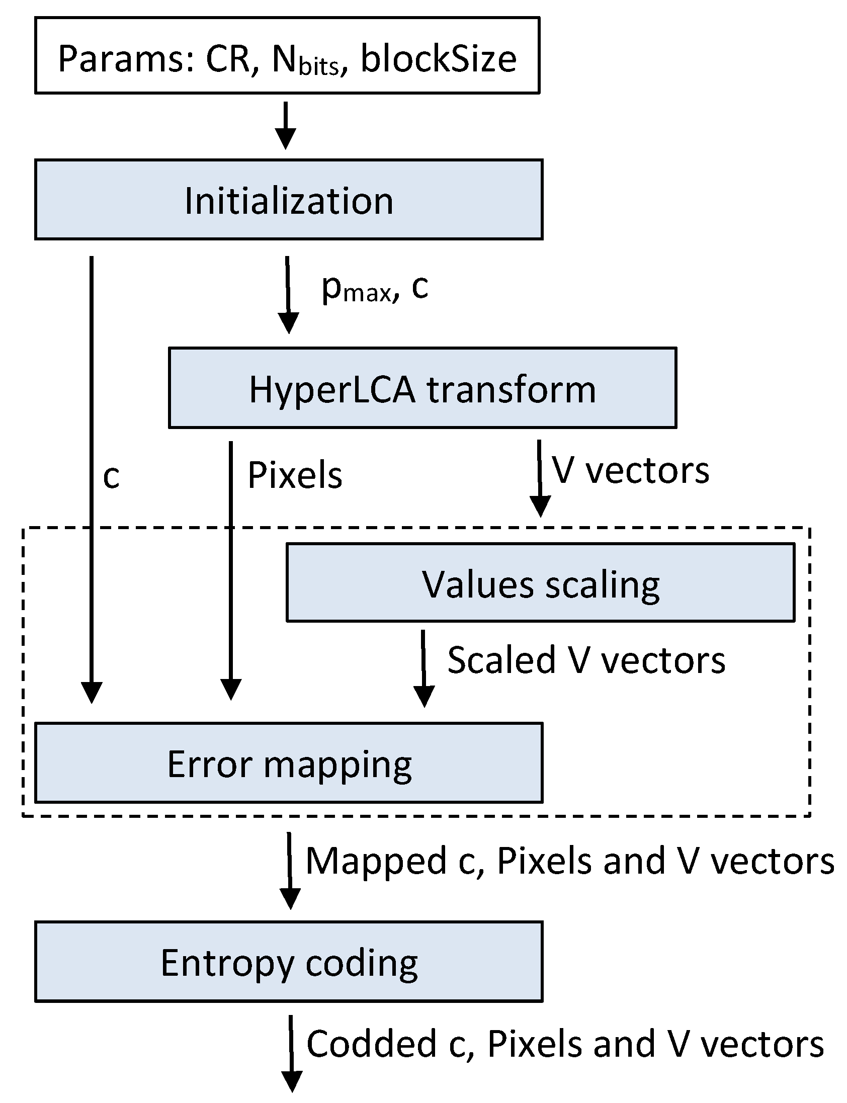
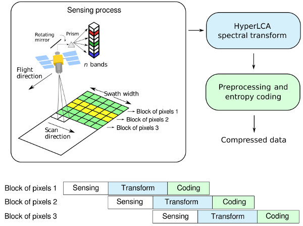
A new transform-based algorithm for performing lossy hyperspectral images compression, named Lossy Compression Algorithm for Hyperspectral image systems (HyperLCA), has been developed in this work with the purpose of providing a good compression performance at a reasonable computational burden. This compression process consists of three main compression stages, which are a spectral transform, a preprocessing stage and the entropy coding stage.
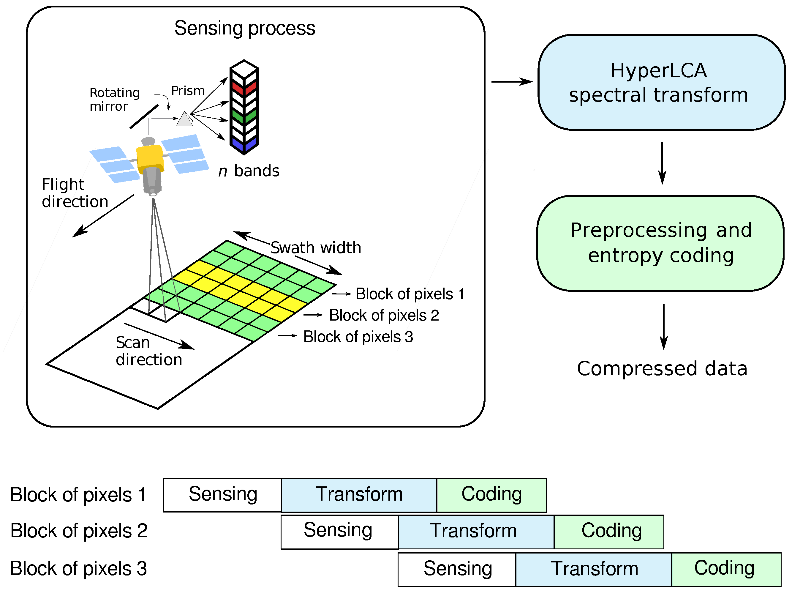
The compression process within the HyperLCA algorithm has been specifically designed for being able to independently compress blocks of pixels of the hyperspectral image without requiring any specific spatial alignment. The goal is to satisfy the requirements of the compression applications that must be executed under tight resources and latency constraints. The possibility of independently compressing blocks of pixels as they are captured avoids the necessity of storing big portions of the image until being able to compress them, reduces the amount of required resources for compressing the collected data, speeds up the process and provides parallelization and error-resilience. One example of application where this strategy may provide important advantages is the remote sensing on-board compression, especially when using pushbroom or whiskbroom sensors.
The most relevant contribution of this work consists in the HyperLCA spectral transform, which allows performing the spectral decorrelation and compression of the hyperspectral data. This transform is able to achieve high compression rate-distortion ratios with a low computational burden and high level of parallelism. The HyperLCA transform selects the most different pixels of the hyperspectral data to be compressed, and then compresses the image as a linear combination of these pixels. The number of selected pixels directly determines the compression ratio achieved in the compression process, and, hence, the compression ratio achieved by the HyperLCA transform can be perfectly fixed as an input parameter. The subsequent preprocessing and entropy coding proposed stages slightly increase the compression ratio achieved by the HyperLCA transform at a very low computational cost and without introducing additional losses of information. A further advantage of this methodology is that, after selecting each of the pixels used for compressing the image, the information that can be represented by the selected pixel is automatically subtracted from the image. Accordingly, the information remaining in the image corresponds with the information that would be lost in the compression–decompression process if no more pixels were selected. This fact enables the possibility of easily providing a stopping condition according to different quality measures such as the Signal-to-Noise Ratio (SNR) or the Maximum Single Error (MaxSE).
The HyperLCA algorithm has been developed also considering how the lossy compression–decompression process affects the ulterior hyperspectral imaging applications. Most of the lossy compression approaches typically behave as low pass filters, which may produce a reduction of the noise present in the image, positively affecting the results when processing the decompressed hyperspectral images in some applications [12]; but, at the same time, the low pass filter can also remove the most atypical elements of the image, which are crucial for several applications, such as anomaly detection, classification, unmixing, or target detection [13,14,15,16,17]. In this scenario, the HyperLCA algorithm provides important advantages with respect to the state-of-the-art solutions. Despite being a lossy compression approach, the HyperLCA algorithm is able to perfectly preserve the most different pixels in the data set through the compression–decompression process and also compresses the rest of the pixels introducing minimal spectral distortions, as it will be demonstrated in this paper.
This paper is organized as follows. Section 2 describes the different compression stages of the HyperLCA algorithm. Section 3 shows the followed methodology for evaluating the goodness of the proposed compressor while Section 4 contains the results obtained in the different accomplished experiments. Finally, Section 5 summarizes the conclusions that have been dragged from this work.

2. Hyperspectral Image Compression within the HyperLCA Algorithm

The HyperLCA algorithm is a lossy transform-based compressor specifically designed for providing a good compression performance at a reasonable computational burden for hyperspectral remote sensing applications. The compression process within the HyperLCA algorithm consists of three main compression stages, which are a spectral transform, a preprocessing stage and the entropy coding stage. Figure 1 graphically shows these three compression stages.
The spectral transform stage, carried on by the HyperLCA spectral transform, performs the spectral decorrelation and compression of the hyperspectral data. The HyperLCA transform is able to achieve high compression rate-distortion ratios with a low computational burden and high level of parallelism. The result of the HyperLCA transform consists of three different sets of vectors, as shown in Figure 1. First of all, a vector with N b components that corresponds with the average pixel of the image or centroid pixel, c, where N b refers to the number of bands of the hyperspectral image. Secondly, the HyperLCA transform also provides a set of vectors of N b components that contains real pixels of the hyperspectral image selected by the transform for being the most different pixels in the data set. This set of pixels vectors is referred to as Pixels in the rest of the manuscript. Finally, the HyperLCA transform provides a set of vectors of N p components, where N p refers to the number of pixels of the image, which allows linearly combining the selected pixels, Pixels, for recovering the real hyperspectral image. This set of vectors is referred as V vectors in the rest of the manuscript.
After performing the HyperCLA transform, the HyperLCA algorithm executes a preprocessing stage followed by an entropy coding stage for slightly increasing the compression ratio achieved by the HyperLCA transform at a very low computational cost and without introducing further losses of information. These two compression stages independently process each of the different Pixels and V vectors as well as the centroid pixel, c. The main goal of the preprocessing stage is to make a very simple prediction of the different vectors’ values, based on the previous value of the specific vector under analysis, and map the prediction error using positive values closer to zero in order to achieve a higher performance in the entropy coding stage. Before the prediction and error mapping, the V vectors are also scaled to positive integer values that perfectly fit the dynamic range produced by the number of bits, N bits defined by the user, as shown in Figure 1. Once that each individual vector is independently preprocessed, its values are entropy encoded using a Golomb–Rice coder [18].
The HyperLCA algorithm has different characteristics that represent important advantages for remote sensing hyperspectral imaging applications. First of all, the compression process within the HyperLCA algorithm has been specifically designed for being able to independently compress blocks of pixels of the hyperspectral image without requiring any specific spatial alignment. The goal is to satisfy the remote sensing on-board compression requirements, especially when using pushbroom or whiskbroom sensors for collecting the images, allowing independently compressing the blocks of pixels as they are captured, as shown in Figure 2. This strategy avoids the necessity of storing large amounts of data until being able to compress them, reduces the amount of required resources for compressing the collected data, speeds up the process and provides parallelization and error-resilience. Additionally, the process performed by the HyperLCA algorithm for compressing each single block of pixels is highly parallel and has a low computational complexity in relation to other state-of-the-art transform-based approaches.
Secondly, the HyperLCA transform selects the most different pixels from the data set. These pixels are preprocessed and coded without losing information and hence they are perfectly preserved through the compression–decompression process. This is one of the most important differences of the HyperLCA algorithm with respect to other state-of-the-art lossy compression approaches, in which the most different pixels are typically lost in the compression. This fact represents a very important advantage for hyperspectral applications such as anomalies detection, target detection, tracking or classification, where it is really important to preserve the anomalous pixels.
Finally, the losses in the compression–decompression process as well as most of the compression ratio obtained are achieved in the spectral transformed stage, carried on by the HyperLCA transform. This provides two more important advantages. On one side, after selecting each of the pixels used for compressing the image (extracting one Pixel vector and its corresponding V vector), the information that can be represented by the selected pixel is automatically subtracted from the image. Accordingly, the information remaining in the image corresponds with the information that would be lost in the compression–decompression process if no more pixels were selected. This fact enables the possibility of easily providing a stopping condition according to different quality measures such as the Signal-to-Noise Ratio (SNR) or the Maximum Single Error (MaxSE). By doing so, if the stopping condition is satisfied, the process finishes and no more Pixels or V vectors are extracted, else, one new Pixel vector is extracted, its corresponding V vector is calculated and the stopping condition is checked again. This procedure also enables a progressive decoding of the compressed bitstream. The image can be reconstructed using just the first Pixels and V vectors in the same order that they are received, and progressively add the information of the subsequent Pixels and V vectors contained in the bitstream if a higher quality is desired.
On the other side, the number of pixels selected by the HyperLCA transform directly determines the compression ratio achieved in the transform stage, and, hence, the minimum compression ratio to be achieved by the HyperLCA transform can be perfectly fixed as an input parameter, ensuring that the compression ratio achieved in the overall process will be always higher (higher means smaller compressed data sets). The compression ratio is defined as CR = (bits real image)/(bits compressed data) in this manuscript, and is used by the HyperLCA transform for determining the maximum number of V vectors and Pixels to be extracted, p max . Once p max Pixels and V vectors have been extracted, the HyperLCA transform finishes, even if the stopping condition based on a quality metric has not been satisfied.
Section 2.1, Section 2.2, Section 2.3, Section 2.4, Section 2.5, Section 2.6, Section 2.7 and Section 2.8 deeply explain each of the different stages of the HyperLCA algorithm for compressing hyperspectral images.

2.1. HyperLCA Input Parameters

The HyperLCA algorithm has three main input parameters that need to be defined.
  • Compression ratio, CR, which indicates the maximum amount of data desired in the compressed image. The HyperLCA algorithm will provide a compressed image at least CR times smaller than the original one.
  • Number of pixels per block, blockSize. This is the number of pixels, with all their hyperspectral bands, to be independently compressed by the HyperLCA algorithm as a single block.
  • Bits for compressed image vectors, N bits . This is the number of bits used for scaling and coding the values of the V = [ v 1 , v 2 , , v p max ] vectors, as described in Section 2.5. The HyperLCA algorithm has been tested in this work using N bits = 16 , N bits = 12 and N bits = 8 .

2.2. HyperLCA Initialization

The HyperLCA algorithm needs to accomplish two main operations before performing the HyperLCA transform according to the characteristics of the image to be compressed and parameters introduced by the user.

2.2.1. Determining the Number of Pixels to be Extracted by the HyperLCA Transform

The compression ratio achieved by the HyperLCA transform is directly determined by the number of extracted vectors and the number of bits used for representing the compressed vectors V = [ v 1 , v 2 , , v p max ] . Accordingly, the maximum number of vectors to be extracted by the HyperLCA transform for each block of pixels, p max , is previously calculated according to the number of bands and the dynamic range of the image to be compressed, and the input parameters, CR, blockSize and N bits as shown in Equation (1), where N p block is the number of pixels per block (blockSize), CR is the minimum compression ratio desired, N bits is the number of bits used for representing the compressed vectors V = [ v 1 , v 2 , , v p max ] , and DR and N b refer to the dynamic range and number of bands of the hyperspectral image to be compressed, respectively:
p max D R · ( N b · ( N p block 1 ) ) C R · ( D R · N b + N bits · N p block ) .
The process can be simplified by using the same precision for representing the compressed vectors V = [ v 1 , v 2 , , v p max ] , N bits , than for representing the image to be compressed, D R , and the Equation (1) would result in Equation (2)
p max N b · ( N p block 1 ) C R · ( N b + N p block ) .

2.2.2. Calculating the Centroid Pixel for Each Block of Pixels

The HyperLCA transform requires the previous calculation of the average or centroid pixel, c, for every block of pixels to be processed. With independence of the data precision used for calculating c, it is rounded to the closest integer value before starting the HyperLCA transform stage. This has two main purposes. First of all, it eases the preprocessing and entropy coding stages, since these two stages need to work with integer values, as described in Section 2.5. Additionally, rounding c to integer values before performing the transformation stage ensures using the exact same vector c in both the HyperLCA transform and inverse transform, which increases the overall accuracy of the compression–decompression process.

2.3. HyperLCA Transform

The HyperLCA transform sequentially selects the most different pixels of the hyperspectral data set. The set of selected pixels is then used for projecting the hyperspectral image, obtaining a spectral decorrelated and compressed version of the data. The compression achieved within this process directly depends on the number of selected pixels. Selecting more pixels provides better decompressed images but lower compression ratios, understanding the compression ratio as the relation between the size of the real image and the compressed one (the higher, the better). Since the pixels are sequentially selected, the sooner the algorithm stops, the higher the compression ratio will be. The proposed method takes advantage of this fact for allowing the user to determine a minimum desired compression ratio, which is used for calculating the maximum number of pixels to be extracted. By doing so, the proposed method ensures the achievement of a compression ratio that will always be higher than the compression ratio specified by the user.
Moreover, each time that a pixel is selected, the information of the image that can be represented using the selected pixel is subtracted from the image. Accordingly, the remaining information directly corresponds with the information that would be lost if no more pixels were selected. This can be used for stopping the sequential extraction of pixels once a specific accuracy level is achieved in the spectral transform step, according to any desired evaluation measurement, without reaching the maximum number of pixels to be extracted, as described in Section 2.8. This way, the proposed method guarantees that if an accurate enough compression of the hyperspectral image is obtained before extracting all the required pixels according to the minimum compression ratio specified by the user, the algorithm will stop, providing a higher compression ratio at a lower computational burden.
Finally, both the extracted pixels as well as information of the image compressed as a linear combination of these pixels are set as the outputs of the HyperLCA transform. This is due to the fact that both are needed for recovering the original hyperspectral image.
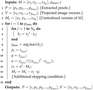
The pseudocode that describes the HyperLCA transform for spectrally decorrelating and reducing the hyperspectral data set is presented in Algorithm 1, where matrix M contains N p real hyperspectral pixels [ r 1 , r 2 , , r N p ] , placed in columns. Each of these pixels is a vector of N b components, N b being the number of bands of the hyperspectral image. The input parameter p max , defined in Section 2.1, determines the maximum number of pixels to be extracted. The input vector c corresponds with the average pixel of the image, also called centroid, in integer values, as described in Section 2.2. Additionally, the set of vectors P = [ p 1 , p 2 , , p p max ] and V = [ v 1 , v 2 , , v p max ] contain the vectors that are extracted by the HyperLCA transform as the compressed information. Specifically, P will store the p max real hyperspectral pixels selected by the HyperLCA transform as the most different pixels of the data set (Pixels), and vectors contained in V will store the information of the image that can be represented by the extracted pixels (V vectors). Each of these vectors has N p components, one per pixel. These vectors are used by the inverse transform for recovering the real image.
First of all, the hyperspectral data, M, is centered and stored in M c , in line 3. This is done by subtracting the centroid pixel to all the pixels of the image. The amount of information present in matrix M c decreases as more pixels are extracted. However, the real image matrix M is not modified.
Secondly, the pixels are sequentially extracted in lines 4–15. In this process, the brightness of each pixel within the M c image is first calculated in lines 5–7. The extracted pixels are selected as those pixels from M that correspond with the highest brightness in matrix M c , as shown in line 9. Then, the orthogonal projection vectors q and u are accordingly obtained as shown in lines 10 and 11.
After that, the information that can be spanned by the defined orthogonal vectors u and q is stored in the projected image vector v p and subtracted from the M c image in lines 12–13. The process finishes when the p max pixels p j have been selected and the information of the image that they can span has been stored in the p max v j vectors, or if an additional stopping condition is previously accomplished, as described in Section 2.8.
This methodology provides one important advantage for compressing and decompressing images for hyperspectral imaging applications. As described in lines 8 and 9 of Algorithm 1, the pixels to be transferred are selected as those with the largest amount of remaining information. By doing this, it is guaranteed that the most different pixels within the data set are perfectly preserved through the spectral decorrelation and compression steps of the compression–decompression process. This fact makes this compression approach especially suitable for applications in which some pixels may be very different from the rest of the pixels, such as anomaly detection, target detection, tracking or classification.
Algorithm 1: HyperLCA transform.
Remotesensing 10 00428 i001

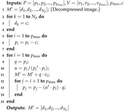
2.4. HyperLCA Inverse Transform

The inverse HyperLCA transform linearly combines the centroid pixel, c, the P = [ p 1 , p 2 , , p p max ] extracted pixels and V = [ v 1 , v 2 , , v p max ] extracted vectors for reconstructing the hyperspectral image, obtaining the decompressed hyperspectral image, M . The pseudocode that describes the inverse HyperLCA transform is presented in Algorithm 2. As shown in lines 2–4 of this pseudocode, all the pixels of M are firstly initialized as the centroid pixel, c. After doing so, the centroid pixel, c, is subtracted to the pixels selected by the HyperLCA transform, as shown in lines 5–7. Finally, the decompressed image, M , is obtained by sequentially adding the result of each of the v i vectors projected using the corresponding orthogonal vector q, as shown in lines 9–11. Lines 12–14 of the pseudocode show how the information that can be represented by the pixels that have been already used ( p i ) is subtracted from the pixels that will be used in the next iterations ( p j = i + 1 to p j = p max ) of the inverse HyperLCA transform.

2.5. HyperLCA Preprocessing

This compression stage of the HyperLCA algorithm is executed after the HyperLCA transform for adapting the output data for being entropy coded in a more efficient way. This compression stage is divided into two different parts.

2.5.1. Scaling the V Vectors

The HyperLCA transform provides two different sets of vectors as a result. These two different sets of vectors, which have different characteristics, are needed for reconstructing the image using the inverse HyperLCA transform, and, hence, both should be entropy coded and transferred. The entropy coder proposed in this manuscript works with integer values. Accordingly, these two sets of vectors must be represented as integers.
Algorithm 2: Inverse HyperLCA transform.
Remotesensing 10 00428 i002
The first set of vectors obtained contains the centroid pixel, c, used for initializing the process, as well as the pixels selected by the HyperLCA transform, P = [ p 1 , p 2 , , p p max ] . The pixels selected by the transform are already integers, since they are directly pixels of the image. The centroid pixel to be transferred has also been rounded to integers’ values before starting the HyperLCA transform, as described in Section 2.2. Accordingly, adapting this set of vectors for the entropy coder is a straightforward step.
On the other hand, the second set of vectors obtained by the HyperLCA transform, V = [ v 1 , v 2 , , v p max ] , contains the projection of the image pixels into the space spanned by the different orthogonal projection vector, u, calculated in each iteration. The value obtained when projecting one pixel vector over one specific vector u will be determined by the angle between both vectors and their magnitude, according to Equation (3), which describes the scalar product between two vectors:
u t · x i = u · x i cos ( θ ) .
According to this equation, larger modules and smaller angles (more parallel vectors) will produce higher scalar product values. In the HyperLCA transform, we have selected the vector u as u = x j max / ( ( x j max ) t · x j max ) , x j max being the brightest pixel in the image (the pixel with the largest magnitude). Hence, if we perform the scalar product of all the image pixels and the u vector as shown in Line 12 of Algorithm 1, v i = u t · M c , the image pixel x j max will be the one producing the largest result, which will be exactly 1, as shown in Equations (4)–(8):
v j max = u t · x j max = ( x j max t ( ( x j max ) t · x j max ) ) · x j max ,
v j max = u t · x j max = ( x j max t x j max 2 ) · x j max ,
v j max = u t · x j max = ( x j max t x j max ) · ( x j max x j max ) ,
v j max = u t · x j max = ( x j max x j max ) · ( x j max x j max ) cos ( θ ) ,
v j max = u t · x i = 1 · 1 cos ( 0 ) = 1 .
Since the rest of the image pixels x j j max have smaller magnitudes than x j max and wider θ angles with respect to the vector u, the values v j j max will be between −1 and 1. Accordingly, it can be said that all the values of the vectors V = [ v 1 , v 2 , , v p max ] will be between −1 and 1, as shown in Equation (9).
v j V : 1 < v j 1
According to this particular property of the vectors V = [ v 1 , v 2 , , v p max ] we can easily scale the v j values for representing them in integer values using all the dynamic range in order to avoid loosing too much precision in the conversion. The v j values are scaled in the HyperLCA algorithm according to the input number of bits , N bits , defined by the user for this purpose, as shown in Equation (10):
v j scaled = ( v j + 1 ) · ( 2 N bits 1 1 ) .
By doing this, it is guarantied that the maximum value obtained for each scaled v j vector is always 2 N bits 1 , and its minimum value is always positive and very close to zero. After rescaling the v j values, they are rounded to the closer integer values so they can be entropy coded.

2.5.2. Represent the Data with Positive Values Closer to Zero

The entropy coding stage takes advantage of the redundancies within the data to be coded, assigning shorter word length to the most common values. In order to achieve higher compression ratios in this stage, the centroid pixel, c, the selected pixels P = [ p 1 , p 2 , , p p max ] , and the already scaled and converted to integer vectors V = [ v 1 , v 2 , , v p max ] , are lossless preprocessed in the HyperLCA algorithm, making use of the prediction error mapper described in the CCSDS recommended standard for lossless multispectral and hyperspectral image compression [19]. This compression stage independently processes each individual vector in order to represent its values using only positive integer values that are closer to zero than the original values of the vector, using the same dynamic range of the values.
Let us assume that we have a vector Y = [ y 1 , y 2 , ] whose components y j are represented using n-bits integers values. In the HyperLCA compressor, this vector Y may be either the centroid pixel, c, a pixel vector p i or a v i vector. Due to the spectral redundancies between contiguous bands, when the vector Y corresponds with a pixel vector p i or the centroid pixel c, we can assume that the difference between the y j and y j 1 components of the vectors is closer to zero than the y j value itself. Similarly, we can make the same assumption when the vector Y corresponds with a v i vector, due to the spatial redundancies of the image. However, in order to prevent bit overflowing in this operation, the number of bits used for representing the prediction error, j = y j y j 1 , needs to be increased to (n+1)-bits, and the values will be in the range ( 2 n + 1 , 2 n 1 ) . In order to solve this issue, the prediction error, j = y j y j 1 , is mapped using the aforementioned prediction error mapper [19].
The overall process works as follows. First of all, the possible minimum and maximum ( y min , y max ) values are calculated as ( 2 n 1 , 2 n 1 1 ) when the vector Y contains negative integer values and ( 0 , 2 n 1 ) when it does not. Then, θ j is calculated as θ j = m i n i m u m ( y j 1 y min , y max y j 1 ) . Finally, the prediction error j = y j y j 1 is mapped according to the j and θ j values as shown in Equation (11):
Y j mapped = 2 j , 0 j θ j , 2 j 1 , θ j j < 0 , θ j + j , otherwise .
By doing this, the values of the centroid pixel, c, the selected pixels P = [ p 1 , p 2 , , p p max ] , and the already scaled and converted to integer vectors V = [ v 1 , v 2 , , v p max ] , are represented using positive values closer to zero, and using the same amount of bits.

2.6. HyperLCA Entropy Coding

After the preprocessing stage of the HyperLCA compressor, the extracted vectors (centroid, Pixels and V vectors) are independently coded using a Golomb–Rice coding strategy. Each single vector is coded as follows:
  • First of all, the compression parameter, M, is calculated as the average value of the vector.
  • Secondly, the lowest power of 2 higher than M, 2 b , is calculated as b = log 2 ( M ) + 1 .
  • Then, each value of the vector is divided by the calculated parameter, M, obtaining the division quotient, q, and the reminder, r.
  • Finally, each value of the vector is coded according to the q and r values obtained, as a code word composed by the quotient code followed by the reminder code.
    -
    The quotient code is obtained by coding the q-value using unary code ( q + 1 bits are required).
    -
    The reminder code is obtained from the r-value. If M is a power of 2, the reminder code is obtained by coding r as plain binary using b bits. If M is not a power of 2, and r < 2 b M , the reminder code is obtained by coding r in plain binary using b 1 bits. In any other situation, the reminder code is obtained by coding r + 2 b M in plain binary using b bits.
The fact of independently coding each vector provides different advantages. On one side, it is possible to use the average value of each vector as the compression parameter, M, which provides almost the best coding performance for the Golomb–Rice method [20], without incrementing too much the complexity of the coder. Nevertheless, in those situations in which calculating the average value of the vector represents an important disadvantage due to its complexity, other solutions could be used, such as the median value, as it is done in other compression algorithms, without compromising its good performance.
On the other side, the fact of independently coding each vector allows coding them in the same order that they are obtained in the previous compression stages of the HyperLCA algorithm. This eases the parallelization of the process, making it possible to pipeline the inputs and outputs of the different compression stages for a single block of pixels, and also reducing the amount of memory required.

2.7. HyperLCA Bitstream Generation

Finally, the outputs of the previous compression stages are packed in the order that they are produced, generating the compressed bitstream. By doing so, the computational requirements for accomplishing this last step of the HyperLCA compressor are minimal. Additionally, this order also eases the decompression process, since the compressed data is used for reconstructing the image in the exact same order that it is produced by the compressor. 
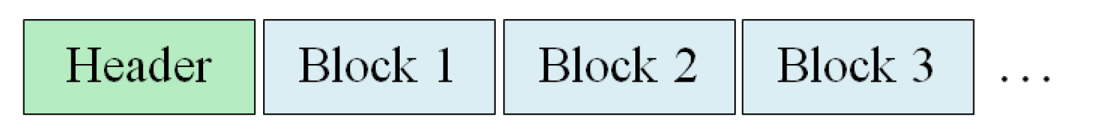
Figure 3 graphically shows the produced bitstream structure.
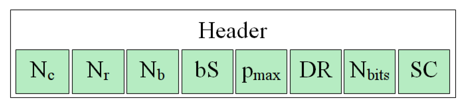
According to Figure 3, the first part of the bitstream is a header that contains the global information about the hyperspectral image and the parameters used in the compression process within the HyperLCA algorithm, which are needed for decompressing the image. Then, the compressed information of each individual block of pixels is packed in the exact same way and sequentially added to the bitstream, as shown in Figure 3.
The information contained in the header of the generated bitstream is:
  • Size of the hyperspectral image, N c , N r and N b , representing the number of columns, rows and bands, coded as plain binary using 16 bits each.
  • The number of pixels per block, blockSize, used for compressing the image within the HyperLCA algorithm, coded as plain binary using 16 bits.
  • The maximum number of V vectors and Pixels extracted for each block of pixels, p max , coded as plain binary using 8 bits.
  • The number of bits needed for covering the entire dynamic range of the hyperspectral image, DR, as well as the number of bits used for scaling the V vectors, N bits , coded as plain binary using 8 bits each.
  • One extra bit, SC, which indicates if one additional stopping condition, based on a quality metric, has been used ( S C = 1 ) or not ( S C = 2 ).
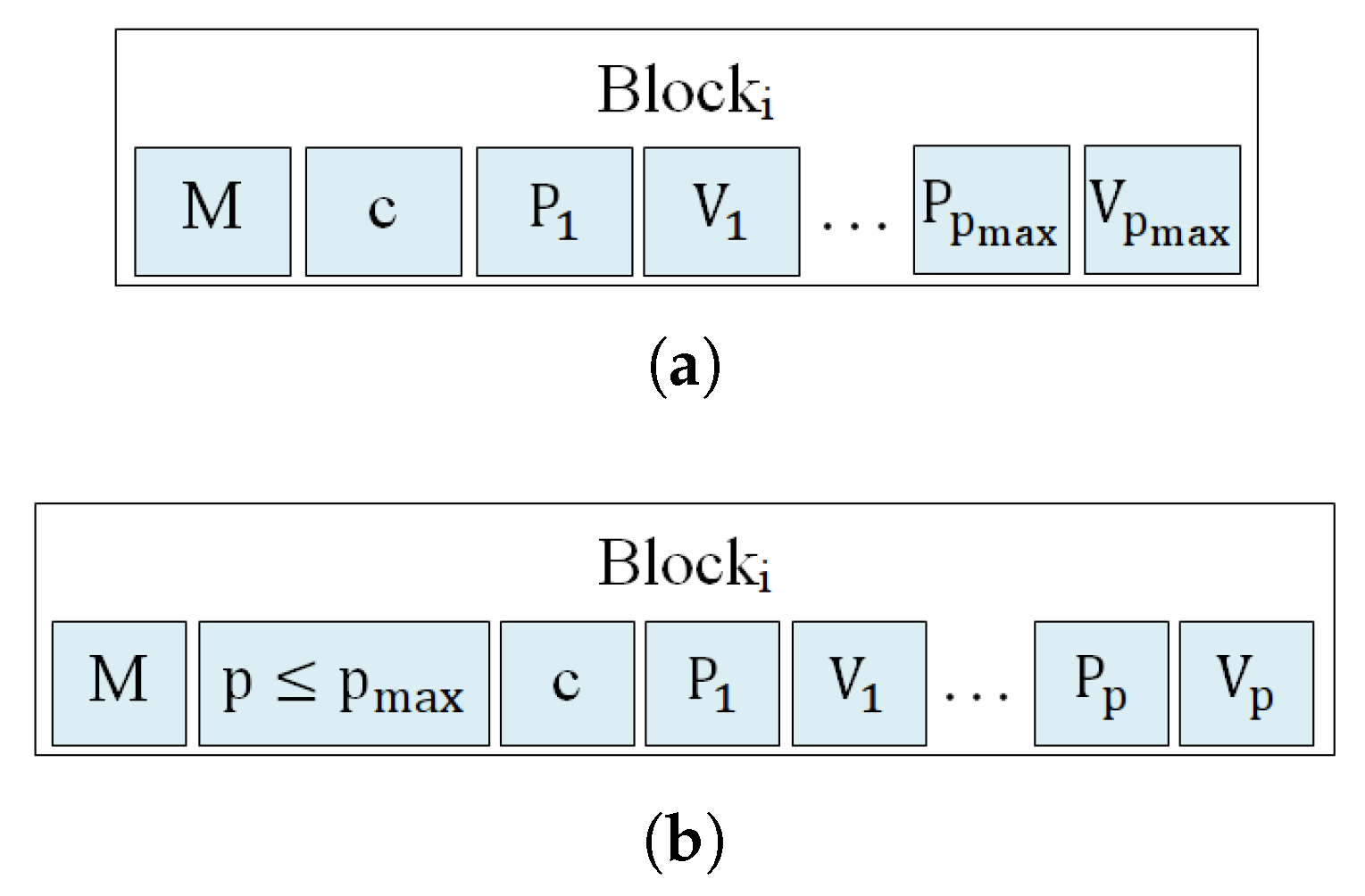
Figure 4 graphically describes the header structure. In this figure, bS represents the number of pixels per block, blockSize. According to the defined number of bits used for the different data contained in the header, 89 bits are required.
The information of each individual block of pixels may be packed in two ways that contain a minimal difference, as shown in Figure 5. The first one, graphically described in Figure 5a, is used when no additional stopping condition is used, and p max Pixels and V vectors are extracted for each individual block. In this situation, the amount of compressed elements in each block is perfectly determined by the p max , N p and N b values that are already included in the bitstream header. On the contrary, when using an additional stopping condition for stopping the algorithm if the desired quality is achieved before extracting p max Pixels and V vectors, the number of Pixels and V vectors extracted for each block of pixels may be different and smaller than p max , producing higher compression ratios. In this situation, the number of Pixels and V vectors used for compressing each block of pixels, p p max , needs to be included when coding each block of pixels, as shown in Figure 5b. This p p max value is coded as plain binary using 8 bits.

2.8. Possible Stopping Conditions within the HyperLCA Algorithm

As previously described, all the losses of the compression–decompression process within the HyperLCA algorithm are produced in the spectral transformation and compression stage, carried on by the HyperLCA transform. As aforementioned, the HyperLCA transform sequentially selects the most different pixels of the image, and uses them for representing the hyperspectral data. Each time that a pixel is selected, the information that can be represented using that specific pixel is subtracted from the image, M c , as described in Line 13 of the Algorithm 1. Accordingly, matrix M c contains the information that would be lost if no more pixels were selected. This information can be used for setting an stopping condition in the sequential pixels selection process, based on the amount of losses desired within the compression–decompression process. For such purpose, two different approaches can be followed:
Global error approaches measure the global or average error in the decompressed image with respect to the original one. Despite these approaches providing a good idea of the accuracy of the compression–decompression process, they do not necessarily yield an accurate reconstruction of the anomalous pixels.
Single error approaches focus on measuring the largest single errors in the decompressed image. Despite these approaches not necessarily providing a very good idea of the overall compression–decompression performance, they are more suitable for verifying the accuracy of the reconstruction of the anomalous pixels.
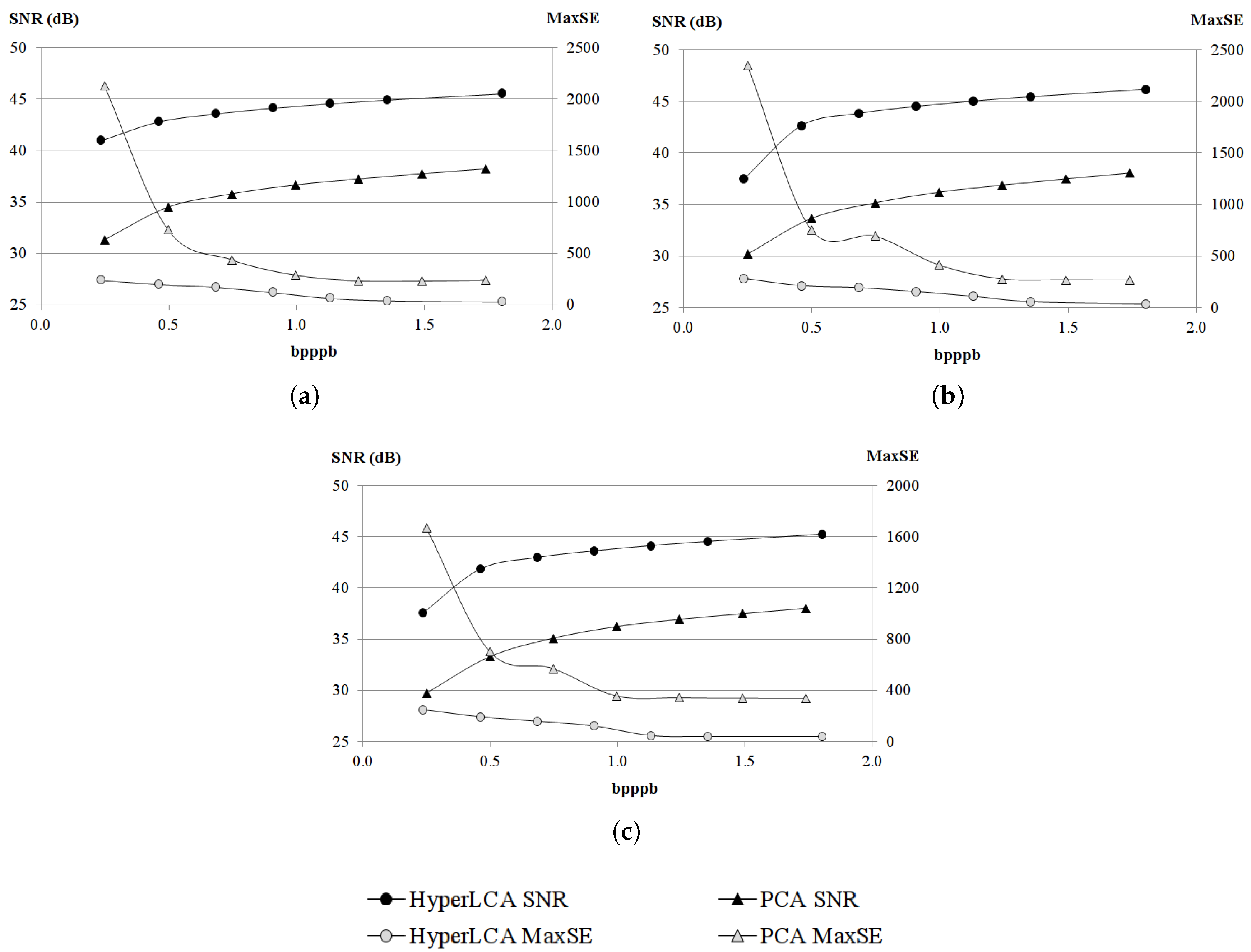
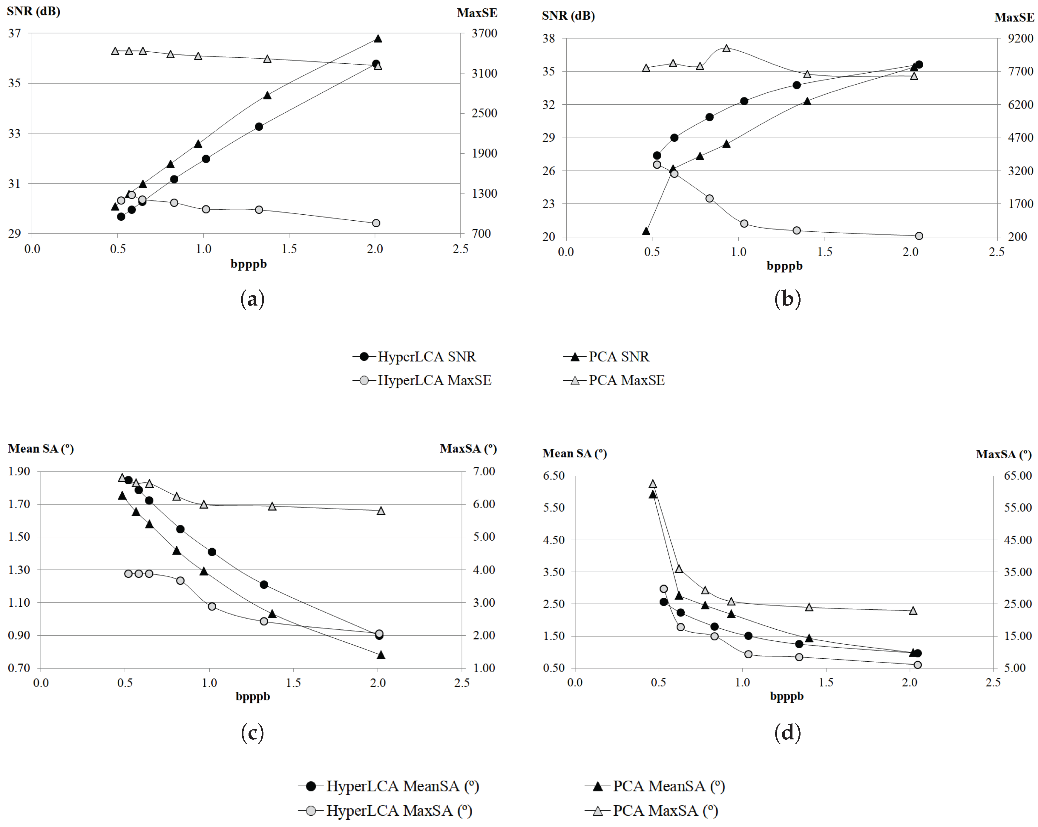
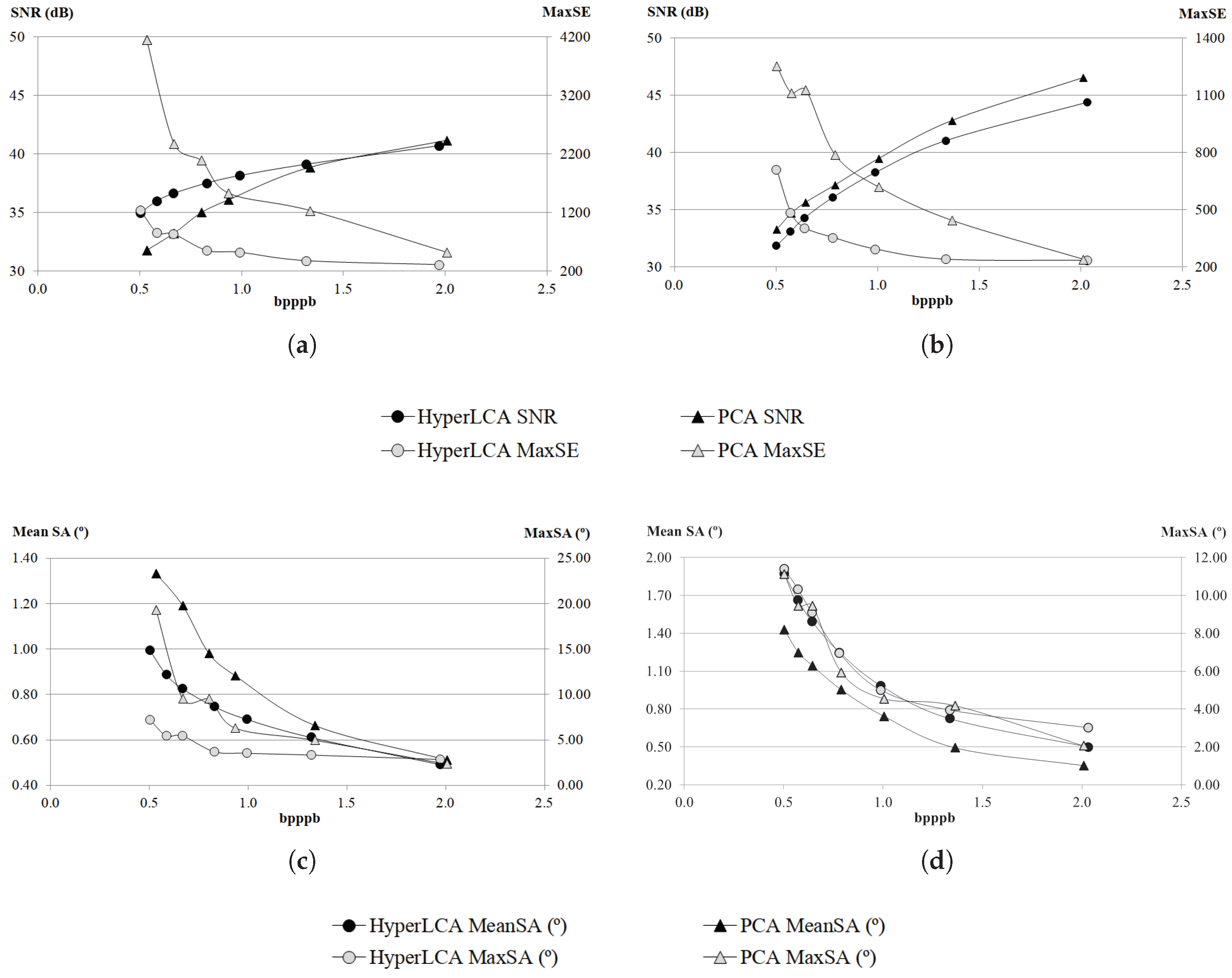
Although many different metrics can be efficiently applied to the proposed HyperLCA transform, we will focus on the RMSE, the SNR and the MaxSE metrics since these are widely used state-of-the-art metrics for evaluating the compression–decompression performance. While the RMSE and SNR are global evaluation metrics that are useful for verifying an average good compression–decompression performance, the MaxSE, despite its simplicity, is more suitable for ensuring that the anomalous pixels are preserved through the compression–decompression process. Any of the possible stopping conditions based on these metrics would be placed in line 14 of the Algorithm 1, and would prevent the extraction of more pixels if the losses achieved are small enough according to the quality metric used.

2.8.1. RMSE Based Stopping Condition

The Root Mean Square Error (RMSE) is a frequently used metric for measuring the average differences between the real hyperspectral image and the decompressed one. A low RMSE represents low average compression–decompression errors. This metric is defined as:
RMSE = 1 N p · N b · i = 1 N b j = 1 N p ( M i , j M i , j ) 2 ,
where M and M refer to the real hyperspectral image and to the decompressed one, and N p and N b refer to the number of pixels and the number of bands in the hyperspectral image, respectively. Since M c contains the information that cannot be represented with the already selected pixels, it could be directly calculated within the HyperLCA algorithm as:
RMSE = 1 N p · N b · i = 1 N b j = 1 N p ( M c i , j ) 2 .

2.8.2. SNR Based Stopping Condition

The Signal-to-Noise Ratio (SNR) generally compares the level of the desired signal to the level of background noise. It is defined as the ratio of signal power to the noise power, often expressed in decibels. In the compression scenario, the SNR metric measures the ratio between the real hyperspectral image power and the compression–decompression loses power, as shown in Equation (14), where M and M refer to the real hyperspectral image and to the decompressed one, and N p and N b refer to the number of pixels and the number of bands in the hyperspectral image, respectively:
SNR = 10 · log 10 ( i = 1 N b j = 1 N p ( M i , j ) 2 i = 1 N b j = 1 N p ( M i , j M i , j ) 2 ) .
As aforementioned, ( M i , j M i , j ) directly corresponds with M c i , j . Hence, the SNR can be calculated within the proposed HyperLCA transform every time that a new pixel is extracted as:
SNR = 10 · log 10 ( i = 1 N b j = 1 N p ( M i , j ) 2 i = 1 N b j = 1 N p ( M c i , j ) 2 ) .
As a further optimization, i = 1 N b j = 1 N p ( M i , j ) 2 can be calculated just once at the beginning of the compression process, since it evaluates just the power of the real hyperspectral image, M.
Finally, it is important to remark that the HyperLCA transform is thought to be independently applied to blocks of pixels of the image, not to the entire image at once. Accordingly, these stopping conditions must be also independently applied to each block of pixels, and, hence, the number of pixels shown in this equations, N p , should be substituted by the number of pixels per block, defined as b l o c k S i z e .

2.8.3. MaxSE Based Stopping Condition

The Maximum Single Error (MaxSE) evaluates the maximum absolute difference between the real hyperspectral image and the compressed-decompressed one. The MaxSE that would be obtained in the compression–decompression process within the HyperLCA algorithm if no more pixels were extracted can be directly calculated, in each iteration, as the maximum absolute value of M c .

2.9. Computational Complexity of the HyperLCA Compressor

The HyperLCA algorithm has been specifically designed for being able to independently compress blocks of pixels of the hyperspectral image without requiring any specific spatial alignment. This fact eases the image compression, especially when using pushbroom or whiskbroom sensors for collecting them, allowing for independently compressing the blocks of pixels as they are captured. This strategy avoids the necessity of storing big portions of the image until being able to compress them, reduces the amount of required resources for compressing the collected data, speeds up the process and provides parallelization and error-resilience. Besides the obvious gains that this fact brings in terms of lower computational complexity, the HyperLCA algorithm has the advantage that it uses simple mathematical operations that can be easily parallelized, avoiding complex matrix operations like, for instance, computing the eigenvalues and eigenvectors, operations that are present in many KLT based compression approaches.
The proposed HyperLCA compressor consists of different compression stages. The first and most computationally demanding one is the HyperLCA transform. This transform spectrally decorrelates each block of pixels of the image and reduces its number of spectral components, according to the specified compression ratio and/or quality measure stopping condition. The amount of data resulting from this transform is already much smaller than the original image. This, together with the simplicity of the subsequent compression stages, makes the computational complexity of these compression stages negligible in relation with the computational burden of the HyperLCA transform. Hence, this section focuses on analysing the computational complexity of the HyperLCA transform.
In order to simplify the analysis of the computational complexity of the HyperLCA transform, the description shown in Algorithm 1 has been followed, considering that no stopping condition based on quality metrics is used, and, hence, the maximum number of pixels to be extracted, p max , is always reached. In particular, the total number of operations done by the HyperLCA transform has been estimated. Despite the fact that the HyperLCA transform can be executed using integer or floating point values, the number of floating point operations (FLOPs) has been considered for simplicity. Additionally, since the HyperLCA transform is independently applied to each block of pixels, the estimation of the number of FLOPs has been done for a single block of N p block pixels. The amount of FLOPs required for processing the entire image directly scales with the number of blocks.
As shown in Algorithm 1, there are three sets of operations that are applied to all the pixels in each of the p max iterations of the HyperLCA transform, and represents the majority of its required FLOPs. These are:
  • The calculation of the amount of remaining information in each pixel by calculating its brightness (lines 5–7 of Algorithm 1). The calculation of the brightness of one pixel corresponds with the inner product between two vectors of N b components, which results in 2 · N b FLOPs. This applied to all the pixels of the block produces a total of 2 · N b · N p block FLOPs.
  • The calculation of the information that can be spanned by the selected pixel, obtaining the corresponding V vector (line 12 of Algorithm 1). This also corresponds with one inner product between two vectors of N b components for each pixel of the image, resulting in 2 · N b · N p block FLOPs.
  • The subtraction of the information that can be spanned by the selected pixel (line 13 of Algorithm 1). This consists of first multiplying the 1 x N p block vector, v i , with the N b x 1 vector, q i , obtaining a N b x N p block , and then subtracting this matrix to the image matrix, M c . Both steps require N b · N p block FLOPs, resulting in a total of 2 · N b · N p block .
The total number of FLOPs required by these three sets of operations is 6 · N b · N p block . Since these operations are done once per each of the p max iterations of the HyperLCA transform, 6 · p max · N b · N p block FLOPs are required for completely processing one block of N p block pixels of N b . Additionally, the p max value depends on the different HyperLCA input parameters, as it is described in Section 2.2. Its exact value can be calculated as shown in Equation (1). Accordingly, the amount of FLOPs to be done by the HyperLCA transform for a single block can be directly estimated from the input parameters as shown in Equation (16):
F L O P s block = 6 · N b · N p block · p max , F L O P s block = 6 · N b · N p block · I n t e g e r ( D R · ( N b · ( N p block 1 ) ) C R · ( D R · N b + N bits · N p block ) ) .
Finally, since the HyperLCA transform is independently applied to each block of pixels, the amount of FLOPs required for processing the entire image can be estimated by multiplying the number of FLOPs required for processing one block by the number of blocks to be compressed. The resulting amount of FLOPs required for processing the entire image withing the HyperLCA transform is shown in Equation (17)
F L O P s Image = 6 · N b · N p · p max F L O P s Image = 6 · N b · N p · I n t e g e r ( D R · ( N b · ( N p block 1 ) ) C R · ( D R · N b + N bits · N p block ) ) .
Different conclusions can be dragged from these expressions. Firstly, it can be observed that higher CR leads to lower p max values, which results in less number of FLOPs required for compressing the image. Additionally, less data is produced by the HyperLCA transform as the CR increases, and, so, less data is to be compressed in the subsequent compression stages. These two facts make the HyperLCA compressor more efficient as the compression ratio increases. Secondly, for the same CR and N b values, smaller block sizes N p block produce smaller p max values, decreasing the number of FLOPs required for compressing the entire image. This makes the HyperLCA compressor more efficient when smaller blocks are used. Additionally, the number of FLOPs required for processing each single block directly depends on the N p block and the p max value, and, hence, the computational complexity (in terms of FLOPs) for independently processing one single block exponentially decreases by decreasing the number of pixels per block, N p block . According to these facts, the HyperLCA compressor would be especially efficient (in terms of FLOPs) for processing hyperspectral images when it is desired to achieve high compression ratios and when using small blocks of pixels. All these facts present important advantages especially when using pushbroom or whiskbroom sensors for collecting the images. The strategy followed by the HyperLCA compressor, based on these facts, avoids the necessity of storing big portions of the image until being able to compress them, reduces the amount of required resources for compressing the collected data, speeds up the process and provides parallelization and error-resilience.
Finally, the operations done by the HyperLCA inverse transform, shown in Algorithm 2, are almost the same as the operations done by the HyperLCA transform, but are used for adding information to the image instead of subtracting it. In general, the operations required for decompressing the image using the HyperLCA algorithm are almost the same as the operations used for compressing it, but applied in reverse order. Due to this reason, the number of FLOPs required for decompressing each block of pixels of the image, as well as the entire image, can be also estimated as shown in Equations (16) and (17), respectively.

2.10. Advantages of the HyperLCA Compression Algorithm

The HyperLCA algorithm has several advantages with respect to other state-of-the-art solutions for lossy compressing hyperspectral images, which will be demonstrated in Section 4 of the current paper. The main advantages of the HyperLCA compressor are detailed next:
  • High compression ratios and decent rate–distortion compression performance.
  • Specially designed for preserving the most different pixels of the data set, which are important for several hyperspectral imaging applications such as anomalies detection, target detection, tracking or classification.
  • The minimal desired compression ratio can be perfectly fixed in advance.
  • Additional stopping conditions can be used for stopping the compression process if the desired quality is achieved at a higher compression ratio than the specified minimum compression ratio.
  • Allows a progressive decoding of the compressed bitstream according to different quality metrics.
  • Low computational complexity and high level of parallelism in relation with other transform-based compression approaches. This eases the hardware implementation of the HyperLCA algorithm for applications under tight latency constraints, also reducing the amount of required hardware resources.
  • Designed for independently compressing blocks of pixels of the image without requiring any spatial alignment between the pixels. This allows starting the compression process just after capturing a block of pixels. This is specially suitable when using pushbroom or whiskbroom hyperspectral sensors.
  • Error resilience. The HyperLCA algorithm independently compresses and codes each block of pixels, and, so, if there is an error in any block of pixels, that error will not affect any other block.
  • The range of values that can be produced by the HyperLCA transform can be perfectly known in advance, which makes it simple to use integer values for representing its results, or for accomplishing all its operations, introducing minimal compression–decompression losses. This eases the integration of the HyperLCA transform with the subsequent compression stages and makes it possible to achieve more efficient hardware implementations.
All these advantages make the HyperLCA algorithm a very suitable option for applications under tight latency constraints or with limited available resources, such as the compression of hyperspectral images on board satellites, where it is critical to consider the amount of power, time and computational resources used.

3. Material and Methods

In order to evaluate the goodness of the proposed HyperLCA algorithm for compressing hyperspectral images in relation with other state-of-the-art approaches for this task, different experiments have been done. The hyperspectral images and quality metrics used in these experiments are detailed next.

3.1. Hyperspectral Images Used

A heterogeneous test bench has been selected in order to evaluate the behavior of the proposed compressor under different circumstances. On one side, we have selected three different images from the well known Airbone Visible/Infrarred Imaging Spectrometer (AVIRIS) [21]. This sensor captures 224 spectral bands in the wavelength range of 400–2500 nm. The first one is the Yellow Stone (Sc 0) radiance image. The other two images used, collected with the AVIRIS sensor, correspond to reflectance images. These are the Lunar Lake image and the Moffet Field one. These images have been cropped to portions of 512 × 512 pixels. Figure 6 graphically shows a false color representation of the portions of the AVIRIS hyperspectral images used.
On the other side, in order to evaluate the behavior of the HyperLCA algorithm in a more challenging scenario, three different uncalibrated images from the Hyperion sensor have been used. The Hyperion sensor produces 242 spectral bands between 355.59 and 2577.08 nm [22]. The Hyperion images that have been used in the experiments are the Erta Ale image, the Lake Monona image and the Mt. St. Helens one. These images have been cropped to portions of 512 × 256 pixels. Figure 7 shows a grey scale representation of these images. As it can be observed in this figure, these images contain a high amount of striping noise, which makes the compression of these images more challenging.
Finally, the impact of the HyperLCA compression process in the ulterior hyperspectral imaging applications has also been evaluated. Specifically, classification, anomaly detection and spectral unmixing applications have been considered. For measuring the effect of the compression process in these applications, some well known images, typically used in these fields due to the existence of their corresponding ground truths, have been selected. These images are preprocessed as it is usually done in the corresponding targeted hyperspectral imaging applications.
First, two different hyperspectral data sets have been used for evaluating the effect of the HyperLCA compression process in classification applications. The first one was collected in 1996 by the AVIRIS sensor over Indian Pines in northwestern Indiana. The selected scene is a total of 145 × 145 pixels with a spatial resolution of 20 m. Bands [1–4], [108–112], [154–167], and 224 have been removed due to water absorption, resulting in a total of 200 hyperspectral bands. The Indian Pines scene contains two-thirds agriculture, and one-third forest or other natural perennial vegetation. There are two major dual-lane highways, a rail line, as well as some low-density housing, other build structures, and smaller roads. The ground truth available is designated into sixteen classes that are briefly summarized in Table 1. The second data set used for evaluating the impact of the HyperLCA compression process in classifications’ applications was captured over the city of Pavia, Italy, by the Reflective Optics Spectrographic Imaging System (ROSIS-03) airborne instrument. The ROSIS-03 sensor has 115 data channels with a spectral coverage ranging from 430 to 860 nm. Twelve channels have been removed due to noise. The data have been corrected atmospherically but not geometrically. The scene consists of 640 × 340 pixels with a spatial resolution of 1.3 m per pixel that covers the Engineering School at the University of Pavia and consists of nine different classes, briefly summarized in Table 1. Figure 8 and Figure 9 show a false color representation of the two described hyperspectral images as well as their corresponding ground truths.
The impact of the HyperLCA compression in anomaly detection applications has been evaluated using two different hyperspectral data sets. The first one was captured over the Rochester Institute of Technology (RIT) by the Wildfire Airborne Sensor Program (WASP) Imaging System [23]. This system covers the visible, short, mid and long-wave infrared regions of the spectrum. The sensor was comprised by a high-resolution colour camera that covers the visible spectrum, a short wave infrared imager that covers from 900 nm to 1800 nm, a mid wave infrared imager that covers from 3000 nm to 5000 nm and a long wave infrared imager that covers from 8000 nm to 9000 nm. In particular, a portion of the overall image, taken over a parking lot, with a size of 180 × 180 pixels and 120 spectral bands, is used in this study. In this scene, the anomalies are fabric targets, which consist of 72 pixels and account for 0.22% of the image. The second data set used was captured by the AVIRIS sensor over the World Trade Center (WTC) area in New York City on 16 September 2001 [24]. A portion of the entire data set, with a size of 200 × 200 pixels and 224 spectral bands, has been used for the tests, where the anomalies are thermal hot spots that consist of 83 pixels and account for 0.21% of the image scene. Figure 10 shows a false color representation of the two described hyperspectral images as well as their corresponding ground truths.
Finally, the Cuprite data set has been used for evaluating the impact of the HyperLCA compression process in unmixing applications. This image was taken by the AVIRIS sensor over the region of Cuprite, Nevada, USA in the summer of 1997. The selected scene consists of a total of 350 × 350 pixels with a spatial resolution of 4 m. Several bands have been removed due to water absorption and low SNR, resulting in a total of 188 spectral bands. The site is well understood mineralogically, and has several exposed minerals of interest including alunite, buddingtonite, calcite, kaolinite and muscovite. The ground truth of this data set consists of the spectral signature of these five minerals, each of them represented in the same 188 spectral bands that the hyperspectral image. Figure 11 graphically shows these five spectral signatures as well as a false color representation of the Cuprite hyperspectral image.

3.2. Evaluation Metrics

Lossy compression approaches for hyperspectral images are typically evaluated in terms of the rate-distortion relation achieved. However, it has been proven that low average distortions in the compression–decompression process do not necessarily ensure good results when the decompressed images are used in specific hyperspectral applications [5]. In general, lossy compression behaves as a low-pass filter, reducing the noise present in the image. This may improve the results obtained in some applications when using the decompressed images. Nevertheless, the low pass filter can also remove the most atypical elements of the image, which are crucial for several applications, such as anomaly detection, classification, unmixing, or target detection [13,14,15,16,17]. Due to this reason, three different evaluation metrics have been used for measuring the goodness of the compression–decompression process within the HyperLCA algorithm. On one side, the Signal-to-Noise Ratio (SNR) has been calculated as already described in Section 2.8.2 for measuring the average looses introduced by the compressor. High SNR values indicate good average compression performance.
On the other side, the Maximum Single Error (MaxSE), already described in Section 2.8.3, has also been used. The maximum single reconstructions errors are typically produced in the most different elements, and, hence, it can be assumed that lower MaxSE values indicate that the most different pixels in the data set are being better preserved through the compression–decompression process [25].
Finally, most of the hyperspectral imaging applications make use of the spectral information of the image for identifying or distinguishing between the different materials present in the scene. Due to this reason, in order to not affect the results of the subsequent hyperspectral applications, it is crucial to preserve the spectral signatures of the pixels through the compression–decompression process, introducing the minimal possible amount of spectral distortions. In order to evaluate the spectral distortions produced by the compression–decompression process within the HyperLCA algorithm, the Spectral Angle (SA) [26], has been used. Lower SA values indicate lower spectral distortions. In particular, the average and maximum spectral distortions have been measured in the experiments by calculating the average and maximum spectral angles between the pixels of the real images and the compressed-decompressed images.
It is important to remark that, although the HyperLCA compressor independently compresses each block of pixels of the image, all these metrics have been calculated for the entire compressed-decompressed images once each single block is decompressed. This allows for making fair comparisons with the other compression approaches used.

4. Results and Discussion

This section discloses the results obtained in all the uncovered experiments with the purpose of evaluating the goodness of the proposed HyperLCA algorithm for compressing hyperspectral images.

4.1. Effect of the Input Parameters of the HyperLCA Compressor

The HyperLCA algorithm has two main input parameters that may affect its compression performance: the number of pixels per block in which the image is divided, blockSize, and the number of bits used for scaling the extracted V vectors, N bits . Different experiments have been done in order to evaluate the behavior of the HyperLCA compressor when using different values for these parameters. In particular, the number of pixels per block, blockSize, has been set to 256, 512 and 1024 pixels, and considering the dynamic range of the AVIRIS and Hyperion sensors, the N bits parameter has been set to 16, 12 and 8 bits for the AVIRIS images and 12 and 8 for the Hyperion sensor images. Figure 12a graphically shows the average rate-distortion obtained, in terms of SNR, when compressing the Lunar Lake hyperspectral image collected by the AVIRIS sensor, according to these parameters for different compression ratios. Figure 12b graphically shows the MaxSE obtained for the same image and compression ratios, according to the different values of blockSize and N bits . Similarly, Figure 13a,b display the same information but for the Erta Ale hyperspectral image collected by the Hyperion sensor.
The achieved compression has been represented in Figure 12 and Figure 13 in terms of Bits per Pixel per Band (bpppb). The bpppb indicates the number of bits of the compressed data in relation with the number of bits of the original image. Accordingly, lower bpppb indicates higher compression ratios, RC.
According to the results shown in Figure 12 and Figure 13 it can be observed that the HyperLCA compressor is able to achieve very high compression ratios with a good rate-distortion relation and low MaxSE values with all the tested combinations of the blockSize and N bits parameters, for both the Lunar Lake AVIRIS image and the Erta Ale Hyperion image. Nevertheless, the best results have been produced when using blocks of 1024 pixels ( b l o c k S i z e = 1024 ). Additionally, the N bits value that has produced the best results is, in average, 12 bits for the Lunar Lake AVIRIS image and 8 bits for the Erta Ale Hyperion image. Hence, in order to verify that these parameters values also produce good compression results for the complete set of images of the AVIRIS and Hyperion sensors, the rest of the images of the data set have been also compressed using the HyperLCA algorithm, using b l o c k S i z e = 1024 and N bits = 12 for the AVIRIS images and b l o c k S i z e = 1024 and N bits = 8 for the Hyperion sensor ones. Figure 14 graphically shows the obtained results. According to these results, the HyperLCA compressor is able to produce relatively high rate-distortion ratios for all the images in the data set, and for very high compression ratios. It is also worth mentioning that the compression performance of the HyperLCA algorithm is very solid for the three different uncalibrated images, collected by the Hyperion sensor, that contain a high amount of striping noise and typically represent a bigger challenge for the compression algorithms. Figure 14 also shows that the MaxSE values tend to very low values for both sensors in relation with their dynamic ranges, also demonstrating the good compression performance of the HyperLCA algorithm.

4.2. Evaluation of the HyperLCA Algorithm against Other Transform-Based Approaches

Most of the advantages of the HyperLCA compression algorithm, described in Section 2.10, are inherited from the HyperLCA transform, explained in Section 2.3. This transform allows to efficiently perform the spectral decorrelation and compression of the hyperspectral image. As aforementioned, the HyperLCA transform has been specially developed for being able to preserve the most different pixels through the compression–decompression process, since these pixels are very important for different hyperspectral imaging applications such as anomalies detection, target detection or classification. In order to verify the goodness of the HyperLCA transform against other state-of-the-art transforms used for the same purpose, the Principal Component Analysis (PCA) has been considered. Despite its computational complexity, the PCA produces some of the best transform-based compression results, in terms of rate-distortion as well as in preserving the relevant information for the ulterior hyperspectral analysis [4,5,6,7].
For making a fair comparison of both hyperspectral transforms, the different hyperspectral images of the data set have been spectrally decorrelated and reduced using the HyperLCA and the PCA transforms, for different compression ratios, without applying any further compression stage. Figure 15, Figure 16, Figure 17 and Figure 18 graphically show the obtained results. It is also worth to mention that while the HyperLCA transform has been computed in order to produce integer values that can be directly processed by the upcoming compression stages, the PCA transform has been computing in Matlab using double precision floating point.
Figure 15 and Figure 16 graphically show the results produced by the HyperLCA and PCA transforms for the different data set images collected by the AVIRIS sensor. Similarly, Figure 17 and Figure 18 show the results obtained with these transforms when processing the images collected by the Hyperion sensor. According to the results shown in Figure 15, both transforms produce similar results in terms of average rate-distortion ratio, the SNR produced by the PCA for these images being slightly better than the SNR produced by the HyperLCA transform. On the contrary, the MaxSE values obtained by the HyperLCA transform for these images are much lower than the MaxSE values obtained by the PCA transform, which indicates that the most different elements are much better preserved when using the HyperLCA transform. Figure 16 corroborates these conclusions. The average rate-distortion relation obtained, evaluated in terms of MeanSA, is similar for both transforms, being slightly better for the PCA transform. However, the MaxSA values obtained in the experiments indicate that there are spectral signatures with higher distortions when using the PCA transform than when using the HyperLCA transform. On the other hand, according to the results obtained when processing the images collected by the Hyperion sensor, shown in Figure 17 and Figure 18, the HyperLCA transform clearly outperforms the PCA transform in terms of SNR, MaxSE and MaxSA, but not in MeanSA.
All these results demonstrate the goodness of the HyperLCA transform for spectrally decorrelating and reducing hyperspectral data sets, and suggest that its results are also good enough when processing images with high levels of noise. The obtained results also verify that the HyperLCA transform is capable of keeping the most different elements of the data set through the compression–decompression process introducing minimal spectral distortions, which makes it very useful when the compressed-decompressed images are to be used for hyperspectral applications such as anomalies detection, target detection, or classification.
Additionally, it can also be observed that the results of the HyperLCA transform, shown in Figure 15 and Figure 17, display similar curves to the results provided by the entire HyperLCA compressor (HyperLCA transform, preprocessor and coder), but at lower compression ratios (higher b p p p b values). This is due to the fact that the HyperLCA preprocessing and coding stages slightly increase the compression ratios achieved by the HyperLCA transform without introducing further compression losses.

4.3. Evaluation of the Impact Produced by the HyperLCA Compression Process in the Ulterior Hyperspectral Imaging Applications

As already mentioned, the HyperLCA algorithm is a lossy compressor for hyperspectral images, especially designed for achieving high compression ratios at a reasonable computational burden. However, it is important to have in mind that the compressed-decompressed data sets have to be useful for the ulterior hyperspectral imaging applications, and, hence, some more requirements need to be fulfilled rather than just achieving a high compression rate–distortion relation. Due to this reason, the HyperLCA algorithm has been specifically designed for preserving the most different pixels of the data set through the compression–decompression process, since these pixels are very important for applications such as anomaly detection, spectral unmixing or classification, as well as for introducing few spectral distortions, since the spectral information is extremely important in most of the hyperspectral imaging applications. Different experiments have been uncovered in this section for evaluating the impact of the HyperLCA compression process in hyperspectral imaging classification, anomaly detection and spectral unmixing applications.
From the entire HyperLCA compression process, all the losses of information are produced by the HyperLCA transform. Due to this reason, the impact of the compression–decompression process using just the HyperLCA transformation stage in the mentioned hyperspectral applications is evaluated and compared with the impact produced by the PCA transform for the same images and applications. It is worth to mention here that the PCA transform is used in many hyperspectral applications, such as unmixing or classification, for spectrally decorrelating the information and reducing the number of spectral components of the data set, with the goal of reducing the redundant information, increasing the separability of the different elements of interest and improving the application results [9,10,27]. Accordingly, the PCA transform can be considered as a good reference to compare with, regarding the impact of the HyperLCA transform in the ulterior hyperspectral applications.

4.3.1. Evaluation of the Impact Produced by the HyperLCA Compression Process in Hyperspectral Imaging Classification

For fairly evaluating the effect of the HyperLCA compressor in hyperspectral imaging classification applications, the Indian Pines and Pavia University data sets, described in Section 3.1, have been spectrally decorrelated and reduced using the HyperLCA and the PCA transforms, for different compression ratios, without applying any further compression stage. Figure 19 graphically shows the obtained performance using both transforms, according to the different evaluation metrics described in Section 3.2. These results have been obtained using blocks of 725 pixels ( b l o c k S i z e = 725 ) for the Indian Pines image, which corresponds to five lines of the image, and blocks of 680 pixels ( b l o c k S i z e = 680 ) for the Pavia University data set, which corresponds to two lines of the image. Additionally, the N bits value has been set to 8 bits for both data sets. After doing so, all the reconstructed images as well as the original images (without applying any transformation) have been classified using the well known Suport Vector Machine (SVM) classifier, which is one of the most widely used classifiers for hyperspectral imaging applications [28]. The SVM classifier has been trained for performing linear prediction following the one versus one classification model, using the LIBSVM tool [29].
The followed methodology is described next:
  • Fifteen samples per class [28] have been randomly selected from the original image (without applying any transformation) for training the SVM classifier. The indexes of the selected samples have been stored for the next steps. After doing so, the rest of the labeled samples have been classified using the generated SVM model, and the Overall Accuracy (OA) has been measured [28]. This is the performance obtained with SVM classifier and the specified configuration for the real data set.
  • The 15 samples per class corresponding to the stored indexes are extracted for each of the reconstructed images, and used for training the SVM classifier for each reconstructed data set, as it was previously done for the original image. These 15 samples may have distortions with respect to the original samples, introduced by the different transforms. The remaining labeled samples of each reconstructed data set have been classified using its corresponding SVM model, generated with its corresponding samples and the exact same configuration that was previously used. Finally, the OA has been measured for each compression ratio and for each of the different applied transforms. This is the performance obtained with the SVM classifier and the specified configuration for each of the reconstructed data sets.
  • Finally, each of the classification maps obtained for each of the reconstructed images have been compared with the classification map obtained with its corresponding original image, calculating the percentage of coincidences (PC).
  • These three steps have been repeated 10 times for each data set for calculating the average results.
The results obtained by following this process are graphically shown in Figure 20 for both the Indian Pines and Pavia University data sets. Each graph displays the OA obtained for each spectral transform and compression ratio (left vertical axis), as well as the PC (right vertical axis). Lower PC values indicate a higher impact of the spectral transform in the classification process (a lossless compression would produce P C = 100 % ). However, the produced impact does not necessarily need to be negative, since the lost information may be removing part of the noise present in the image, which could improve the classification results, or relevant information, which would decrease the classification performance [12]. When the OA values obtained with the reconstructed images are higher than the OA values obtained with the original image, it indicates a positive impact of the transform. On the contrary, when the OA values obtained with the reconstructed images are lower than the OA values obtained with the original image, it indicates a negative impact. The horizontal dashed line displayed in both graphs shows the OA obtained with the original Indian Pines and Pavia University images.
Different conclusions can be dragged from the results shown in Figure 20. First of all, according to the obtained PC, it can be observed that the HyperLCA transform produces a lower impact in the classifier than the PCA transform, for both data sets, with independence of the compression ratio achieved. It can also be seen that the PC obtained using both transforms decreases as the compression ratio increases (smaller b p p p b ), which makes sense considering that the amount of losses introduced by the transforms increase with the compression ratio.
Regarding the OA obtained in the experiments, it can be observed that better classification results are obtained when using the HyperLCA transform than when using the PCA transform, when using the SVM classifier with the specified configuration and the two described data sets. It can also be observed that the OA obtained for the images processed using the PCA transform are always lower than the OA obtained for the original images, and decreases when the compression ratio increases. This suggests that part of the important information present in the original image is lost when using the PCA transform, and these losses are higher when the compression ratio increases. On the contrary, the OA obtained for the images processed using the HyperLCA transform tends to be higher than the OA obtained for the original images. This suggests that the information lost when using the HyperLCA transform is not relevant for the SVM classification process, and that these losses help to maximize the differences between the samples of the different classes.
According to these results, it could be considered that the HyperLCA transform has a smaller and more positive impact than the PCA transform in the ulterior hyperspectral imaging classification.

4.3.2. Evaluation of the Impact Produced by the HyperLCA Compression Process in Hyperspectral Anomaly Detection

For fairly evaluating the effect of the HyperLCA compressor in hyperspectral anomaly detection applications, the Rochester Institute of Technology (RIT) and the World Trade Center (WTC) data sets, described in Section 3.1, have been spectrally decorrelated and reduced using the HyperLCA and the PCA transforms, for different compression ratios, without applying any further compression stage. Figure 21 graphically shows the obtained performance using both transforms, according to the different evaluation metrics described in Section 3.2. These results have been obtained using blocks of 1080 pixels ( b l o c k S i z e = 1080 ) for the RIT image, which corresponds to six lines of the image, and blocks of 1000 pixels ( b l o c k S i z e = 1000 ) for the WTC data set, which corresponds to five lines of the image. Additionally, the N bits value has been set to 8 bits for both data sets. After doing so, all the reconstructed images as well as the original images (without applying any transformation) have been processed using the well known Orthogonal Subspace Projection Reed-Xiaoli (OSPRX) detector for identifying the anomalous pixels. The OSPRX algorithm is one of the commonly used detectors for anomaly detection applications and provides good detection results [30,31,32].
The followed methodology is described next:
  • The RIT and WTC original images (without applying any transformation) have been first processed using the OSPRX detector. This detector requires specifying the number of bands to use for representing the image information considered as background. This number has been set to 4 in the experiments, since this value produces very good anomaly detection results for both data sets [33]. By doing so, two anomaly maps have been obtained, one per image.
  • The accuracy of the detection results using the original images has been evaluated using the Receiver Operating Characteristics (ROC) curves, and more specifically, the area under these curves (AUC) [30]. The ideal AUC value is 1. Lower AUC values indicate poorer detection performance. The obtained AUC values are 0.9837 and 0.9983 for the RIT and WTC data sets, respectively.
  • The same process has been followed for each of the reconstructed images, also setting to 4 the input number of bands used by the OSPRX detector. By doing so, one anomaly map and AUC value are obtained for each image, transform and compression ratio achieved.
  • Finally, each of the anomaly maps generated for each of the reconstructed images has been compared with the anomaly maps obtained with the original images, calculating the Mean Square Error (MSE) between the anomaly maps.
The results obtained by following this process are graphically shown in Figure 22 for both the RIT and WTC data sets. Each graph displays the AUC values obtained for each spectral transform and compression ratio (left vertical axis), as well as the MSE obtained for the different anomaly maps, corresponding to the reconstructed images (right vertical axis). Higher MSE values indicate a bigger difference between the anomaly maps generated with the reconstructed images and the one generated with the original image, which means a higher impact of the HyperLCA and PCA transforms in the anomaly detection process. This impact could be positive if just part of the noise present in the image is removed by the transforms, which could improve the anomaly detection results, or negative if relevant information, such as the anomalous pixels, is lost [12]. When the AUC values obtained with the reconstructed images are closer to 1 than the AUC value obtained for the original image, it indicates a positive impact of the transform. On the contrary, when the AUC values obtained with the reconstructed images are closer to 0 than the AUC values obtained with the original image, it indicates a negative impact. The horizontal dashed line displayed in both graphs shows the AUC value obtained with the original RIT and WTC images.
Different conclusions can be dragged from the results shown in Figure 22. First of all, according to the obtained MSE, it can be observed that the HyperLCA transform produces a lower impact in the anomaly detection process within the OSPRX detector than the PCA transform, for both data sets, with independence of the compression ratio achieved. It can also be seen that the MSE obtained using both transforms increases with the compression ratio (smaller b p p p b ), which makes sense considering that the amount of losses introduced by the transforms also increases with the compression ratio. It is also appreciable that the MSE values obtained are very close to 0. This is due to the fact that the anomaly maps should provide values close to 0 for the background pixels and values close to 1 for the anomalous pixels. Accordingly, most of the values obtained in the anomaly maps are very close to 0. Since the amount of anomalous pixels represents less than the 0.25 % in both images, anomaly maps with big errors in the anomalous pixels would still produce very small MSE values. Hence, it is important to have in mind that low MSE values when comparing the obtained anomaly maps do not necessarily mean a low impact of the transforms in the anomaly detection process, and that this metric can be used just as a comparative between both transforms.
Regarding the AUC values obtained in the experiments, it can be observed that better anomaly detection results are obtained when using the HyperLCA transform than when using the PCA transform, when using the OSPRX detector with the specified configuration and the two described data sets. It can also be observed that the AUC values obtained when using the compressed-decompressed RIT image, using both transforms, are better than the results obtained when using the original image. This suggests that the important information for the anomaly detection is preserved by both transforms and that just part of the noise or not useful information (for anomaly detection and the OSPRX detector) has been removed. It is also interesting that, for the RIT data set, the OSPRX performance increases with the compression ratio (higher AUC values are obtained for lower bpppb), for both spectral transforms. However, for the WTC data set, the OSPRX performance obtained with the compressed-decompressed image using the PCA transform significantly decreases for the highest compression ratios. This suggests that at such high compression ratios, the anomalous pixels have been lost through the PCA compression process.
According to these results, it could be considered that both spectral transforms are able to preserve the anomalous pixels through the compression–decompression process, having a positive impact in the anomaly detection process when using the OSPRX detector, at least for a wide range of compression ratios and the two selected data sets. It could also be concluded that the results obtained by the OSPRX detector are better when the HyperLCA transform has been applied rather than when the PCA transform has been applied.

4.3.3. Evaluation of the Impact Produced by the HyperLCA Compression Process in the Endmembers Finding Process for Spectral Unmixing Applications

The effect of the HyperLCA compressor in endmembers finding applications has been evaluated using the Cuprite data set, described in Section 3.1. This hyperspectral image has been spectrally decorrelated and reduced using the HyperLCA and the PCA transforms, for different compression ratios, without applying any further compression stage. Figure 23 graphically shows the obtained performance using both transforms, according to the different evaluation metrics described in Section 3.2. The HyperLCA results have been obtained using blocks of 700 pixels ( b l o c k S i z e = 700 ), which corresponds to two lines of the image, and setting the N bits value to 8 bits.
After spectrally decorrelating and reducing the Cuprite image for the different compression ratios, using both transforms, all the reconstructed images as well as the original one (without applying any transformation) have been analysed in order to identify the pixels of the data set with the smallest differences in relation to the five pure spectral signatures of the ground truth: alunite, buddingtonite, calcite, kaolinite and muscovite. This allows identifying the pixels that would be the best candidates of each image to be selected as endmembers by spectral linear unmixing algorithms based on pure pixels [11], such as the Vertex Component Analysis (VCA) [34], the Orthogonal Subspace Projection (OSP) [35] or N-Finder [36] algorithms, among others. The best performance that the mentioned unmixing algorithms could achieve when processing the different compressed-decompressed images, as well as the original one, can be evaluated attending to the spectral angle obtained for the pixels identified as the best candidates to be endmembers. Lower spectral angle values indicate better achievable performance. The MeanSA and MaxSA values obtained for these pixels in the Cuprite image, when using both transforms and different compression ratios are graphically shown in Figure 24. The MeanSA and MaxSA values obtained for the original Cuprite image are also displayed in this graph as dashed lines.
The results displayed in Figure 24 show that the effect of the HyperLCA transform in the SA values obtained does not vary too much with the compression ratio achieved. This suggests that the HyperLCA transform could have a low impact in the results of the unmixing applications. On the other hand, the SA values obtained when using the PCA transform present larger variations for the different compression ratios, which suggests that the PCA transform has a higher impact on the achievable results of the ulterior unmixing applications. Nevertheless, the results obtained when using any of the tested transforms are very similar to the results obtained when using the Original Cuprite image, indicating that the impact produced by these transforms in the ulterior spectral unmixing applications could be negligible.

4.4. Evaluation of the HyperLCA Algorithm against the State-of-the-Art Solutions for on-Board Applications

Finally, as described in Section 1, the HyperLCA algorithm has been designed with the purpose of offering a hardware-friendly transformed based approach for lossy compressing hyperspectral images. The main goal is to provide a new solution for applications with limited available resources, such as compression on-board satellites. In particular, this new solution focuses on obtaining high compression ratios at a reasonable rate-distortion relation, without compromising too much the ulterior hyperspectral imaging applications.
This section is devoted to evaluating the characteristics of the HyperLCA compressor against the state-of-the-art solutions for on-board hyperspectral imaging compression, and, more specifically, against the actual standards proposed by the Consultative Committee for Space Data Systems [19] for space applications. The goal is to verify that the HyperLCA algorithm provides some new advantages for some specific situations and/or applications that are not totally covered by the existing standards.
The CCSDS has published two standards specially focused on hyperspectral imaging compression (also applicable to multispectral image compression). These are the CCSDS122.1-B-1 Spectral Preprocessing Transform for Multispectral and Hyperspectral Image Compression [37] and the CCSDS123.0-B-1 Lossless Multispectral and Hyperspectral Image Compression [38].
The CCSDS122.1-B-1 proposes a compressor that consists of two main functional parts: a spectral transform and a set of 2D encoders. The proposed 2D coders extend the (two-dimensional) CCSDS Image Data Compression standard, CCSDS 122.0-B-2 [39]. The process consists of first spectrally decorrelating the data set using one of the three proposed spectral transforms: the Integer Wavelet Transform (IWT) [40], the Pairwise Orthogonal Transform (POT) [41,42] or the Arbitrary Affine Transform (AAT), and, then, independently compressing each of the decorrelated image bands using the mentioned two-dimensional coder. The CCSDS122.1-B-1 also allows using the Identity Transform instead of any of the mentioned transforms. This transform is defined for the sake of providing a compressed data structure to encode a 3D image without requiring the implementation of a more complex transform stage. The compressor proposed in the CCSDS122.1-B-1 standard may produce both lossless or lossy hyperspectral image compression. However, the losses are mostly introduced by the 2D CCSDS 122.0-B-2 image coder, the spectral transform being mainly executed as lossless transforms. The AAT is the only one of the mentioned transforms that is not guaranteed to produced lossless results. In this sense, the HyperLCA compressor proposes a different strategy, the HyperLCA transform being the one taking control of the introduced losses while the subsequent HyperLCA compression stages produce lossless compression. This represents an additional computational advantage for the HyperLCA compressor, since the amount of data to be coded by the compression stages that goes after the HyperLCA transform is much smaller than the original image. On the contrary, when following the strategy proposed in the CCSDS122.1-B-1, the amount of information to be coded after applying the spectral transforms is exactly the same size as the original image. The equivalent approach using the transforms proposed in the CCSDS122.1-B-1 standard would be to preserve just a certain number of the decorrelated bands for reconstructing the hyperspectral image, and lossless compressing these bands using the CCSDS 122.0-B-2 coder. The information contained in the bands that are not considered would correspond with the losses produced in the compression process. However, even doing it this way, it would not exactly correspond with the strategy followed by the HyperLCA algorithm, since, in this approach, the spectral transform would being applied to the entire image at once, while the HyperLCA transform is independently applied to a subset of pixels of the image (typically one or some lines of the image).
Nevertheless, the transform-based compression approach proposed by the CCSDS122.1-B-1 is the most similar to the HyperLCA compression strategy from all the CCSDS standards. As it is described in this standard, the Karhunen Loève Transform (KLT) is “the transform that provides perfect decorrelation”, and the POT is an approximation of the (KLT) at a fraction of its computational cost. The standard also describes that, in general, the POT provides better coding performance than the IWT, but requires more computational resources and has a more complex implementation. Additionally, these assertions are empirically demonstrated in [5,7,41,42,43]. These results show that the compression performance of the KLT transform (PCA) clearly surpasses the compression performance provided by the rest of the transforms contained in the aforementioned standard. Accordingly, the results shown in the previous sections of this manuscript, where the results provided by the HyperLCA transform are widely compared with the results provided by the PCA transform, for different images and compression ratios, should be enough for verifying the good behavior of the HyperLCA transform for lossy compressing hyperspectral images, particularly when high compression ratios are desired. It is also important to remark here that the HyperLCA compressor has been specifically developed for lossy compressing hyperspectral images and, hence, its efficiency is not guaranteed for compressing multispectral images (with few bands), or for lossless compressing hyperspectral images.
On the other hand, the CCSDS123.0-B-1 proposes a 3D lossless prediction-based compression algorithm for hyperspectral images, which is hardly optimized for producing an efficient lossless compression at a relatively low computational cost. However, as any other lossless compressor, its achievable compression ratio is limited [44,45,46]. The authors consider that the use of a lossy transform-based approach, such as the HyperLCA compressor, which may be more complex that the compressor described in this standard, is only justified when it is important to achieve high compression ratios that are not achievable by the CCSDS123.0-B-1 compressor. Hence, the maximum compression ratios achieved by this compressor for the data sets described in Section 3.1 are shown in Table 2. Table 2 also shows different rate-distortion relations achieved by the HyperLCA compressor for the same images. The HyperLCA results shown in this table have been obtained using 1024 pixels per block ( b l o c k S i z e = 1024 ) and setting the N bits parameter to 12 and 8 for the images collected by the AVIRIS and Hyperion sensors, respectively. The CCSDS123.0-B-1 results have been obtained using the WhiteDwarf software [47], developed by the European Space Agency (ESA). Additionally, an RGB representation of the compressed-decompressed AVIRIS images corresponding to Table 2 are displayed in Figure 25. Similarly, a grey scale representation of the compressed-decompressed Hyperion images corresponding to Table 2 are displayed in Figure 26. Figure 25 demonstrates that no appreciable spatial errors are introduced in the images collected by the AVIRIS sensor when compressing them using the HyperLCA algorithm, since the RGB images obtained for the different compression ratios seem very similar. However, there are some spatial differences in the compressed-decompressed images obtained for the Hyperion sensor, as can be observed in the Figure 26, especially for the highest compression ratios shown in Table 2. It seems that the striping noise is slightly removed, but also that some lines of the images are blurred (just for the highest compression ratios). Nevertheless, these results seem pretty good considering the quality of the Hyperion images and the achieved compression ratios.
The obtained results verify that the HyperLCA compressor is able to achieve much higher compression ratios (lower bpppb) than the CCSDS123.0-B-1 compressor at a reasonable good rate-distortion relation. This, together with the other features of the HyperLCA algorithm, makes this proposal a suitable option for those applications, where it is desired to perform lossy compression with the purpose of achieving high compression ratios (less than 2 b p p p b ).

5. Conclusions

In this manuscript, a new transform-based algorithm for performing lossy hyperspectral images compression, named Lossy Compression Algorithm for Hyperspectral image systems (HyperLCA), has been proposed. The main goal of this compressor is to provide a good compression performance at a reasonable computational burden, especially for very high compression ratios that are hardly achievable by lossless compression approaches. The proposed HyperLCA algorithm has different advantages. First of all, it is able to achieve high compression ratios while preserving the most different elements of the data set, which are crucial for many hyperspectral images applications such as anomaly detection, target detection or classification. Secondly, the compression ratio to be achieved can be perfectly fixed in advance. Additionally, some extra stopping conditions, based on quality metrics, can be added in order to stop the compression if the desire minimal quality is achieved at higher compression ratios than the specified. The possibility of adding these kinds of stopping conditions also enables a progressive decoding of the compressed bitstream. Furthermore, the HyperLCA algorithm is able to independently compress blocks of pixels of the image, increasing its error resilience and making it specially suitable for applications that use pushbroom or whiskbroom sensors. Finally, the HyperLCA also has many computational advantages, including low mathematical complexity and a high level of parallelism, which differentiate it from other state-of-the-art transform-based compression approaches and make it a more viable option for applications under tight latency constraints or applications with limited computational resources, such as hyperspectral compression on-board satellites.
An extensive amount of experiments have been performed in order to evaluate the goodness of the proposed HyperLCA compressor using different calibrated and uncalibrated hyperspectral images from the AVIRIS and Hyperion sensors. The results provided by the proposed HyperLCA compressor have been evaluated and compared against those produced by some of the most relevant state-of-the-art compression solutions. Additionally, the effect produced by compressing-decompressing the image using the HyperLCA transform in anomaly detection, hyperspectral imaging classification and spectral unmixing applications has also been evaluated. All the obtained results allow to conclude that the proposed HyperLCA compressor represents a very suitable option for lossy compressing hyperspectral images, especially when it is important to achieve high compression ratios while at the same time preserving the most different elements of the data set, and when it is important to perform the compression under tight latency and computational constraints.

Acknowledgments

This research is partially funded by the European Commission through the ECSEL Joint Undertaking (ENABLE-S3 project, No. 692455) and the Ministry of Economy and Competitiveness (MINECO) of the Spanish Government (ENABLE-S3 project, No. PCIN-2015-225 and REBECCA (Resilient EmBedded Electronic systems for Controlling Cities under Atypical situations) project, No. TEC2014-58036-C4-4-R.

Author Contributions

Raúl Guerra, Yubal Barrios, María Díaz, Lucana Santos, Sebastián López and Roberto Sarmiento were all involved in the study, design and writing of this paper. Raúl Guerra and María Díaz carried out the development of the HyperLCA compressor. Lucana Santos provided reference software and knowledge about the state-of-the-art solutions for on-board compression. Yubal Barrios performed the experiments. Sebastián López and Roberto Sarmiento supervised the work and revised the manuscript.

Conflicts of Interest

The authors declare no conflict of interest.

References

  1. Penna, B.; Tillo, T.; Magli, E.; Olmo, G. Progressive 3-D coding of hyperspectral images based on JPEG 2000. IEEE Geosci. Remote Sens. Lett. 2006, 3, 125–129. [Google Scholar] [CrossRef]
  2. Chang, L.; Cheng, C.M.; Chen, T.C. An efficient adaptive KLT for multispectral image compression. In Proceedings of the 4th IEEE Southwest Symposium on Image Analysis and Interpretation, Austin, TX, USA, 2–4 April 2000; pp. 252–255. [Google Scholar]
  3. Hao, P.; Shi, Q. Reversible integer KLT for progressive-to-lossless compression of multiple component images. In Proceedings of the 2003 International Conference on Image Processing, Barcelona, Spain, 14–17 September 2003; Volume 1. [Google Scholar]
  4. Amrani, N.; Serra-Sagristà, J.; Laparra, V.; Marcellin, M.W.; Malo, J. Regression wavelet analysis for lossless coding of remote-sensing data. IEEE Trans. Geosci. Remote Sens. 2016, 54, 5616–5627. [Google Scholar] [CrossRef]
  5. Penna, B.; Tillo, T.; Magli, E.; Olmo, G. Transform coding techniques for lossy hyperspectral data compression. IEEE Trans. Geosci. Remote Sens. 2007, 45, 1408–1421. [Google Scholar] [CrossRef]
  6. Du, Q.; Zhu, W.; Fowler, J.E. Anomaly-based hyperspectral image compression. In Proceedings of the IGARSS 2008. IEEE International Conference on Geoscience and Remote Sensing Symposium, Boston, MA, USA, 6–11 July 2008; Volume 2. [Google Scholar]
  7. Du, Q.; Fowler, J.E. Hyperspectral image compression using JPEG2000 and principal component analysis. IEEE Geosci. Remote Sens. Lett. 2007, 4, 201–205. [Google Scholar] [CrossRef]
  8. Taubman, D.; Marcellin, M. JPEG2000 Image Compression Fundamentals, Standards and Practice: Image Compression Fundamentals, Standards and Practice; Springer Science & Business Media: New York, NY, USA, 2012; Volume 642. [Google Scholar]
  9. Bioucas-Dias, J.M.; Plaza, A.; Camps-Valls, G.; Scheunders, P.; Nasrabadi, N.M.; Chanussot, J. Hyperspectral remote sensing data analysis and future challenges. IEEE Geosci. Remote Sens. Mag. 2013, 1, 6–36. [Google Scholar] [CrossRef]
  10. Bioucas-Dias, J.M.; Plaza, A.; Dobigeon, N.; Parente, M.; Du, Q.; Gader, P.; Chanussot, J. Hyperspectral unmixing overview: Geometrical, statistical, and sparse regression-based approaches. IEEE J. Sel. Top. Appl. Earth Obs. Remote Sens. 2012, 5, 354–379. [Google Scholar] [CrossRef]
  11. Blanes, I.; Serra-Sagrista, J.; Marcellin, M.W.; Bartrina-Rapesta, J. Divide-and-conquer strategies for hyperspectral image processing: A review of their benefits and advantages. IEEE Signal Process. Mag. 2012, 29, 71–81. [Google Scholar] [CrossRef]
  12. Santos, L.; López, S.; Callico, G.M.; López, J.F.; Sarmiento, R. Performance evaluation of the H. 264/AVC video coding standard for lossy hyperspectral image compression. IEEE J. Sel. Top. Appl. Earth Obs. Remote Sens. 2012, 5, 451–461. [Google Scholar] [CrossRef]
  13. Aiazzi, B.; Alparone, L.; Baronti, S. Quality issues for compression of hyperspectral imagery through spectrally adaptive DPCM. In Satellite Data Compression; Springer: New York, NY, USA, 2012; pp. 115–147. [Google Scholar]
  14. Lee, C.; Lee, S.; Lee, J. Effects of lossy compression on hyperspectral classification. In Satellite Data Compression; Springer: New York, NY, USA, 2012; pp. 269–285. [Google Scholar]
  15. García-Vílchez, F.; Muñoz-Marí, J.; Zortea, M.; Blanes, I.; González-Ruiz, V.; Camps-Valls, G.; Plaza, A.; Serra-Sagristà, J. On the impact of lossy compression on hyperspectral image classification and unmixing. IEEE Geosci. Remote Sens. Lett. 2011, 8, 253–257. [Google Scholar] [CrossRef]
  16. Du, Q.; Ly, N.; Fowler, J.E. An operational approach to PCA+ JPEG2000 compression of hyperspectral imagery. IEEE J. Sel. Top. Appl. Earth Obs. Remote Sens. 2014, 7, 2237–2245. [Google Scholar] [CrossRef]
  17. Chang, C.I. Hyperspectral Data Processing: Algorithm Design and Analysis; John Wiley & Sons: Hoboken, NJ, USA, 2013. [Google Scholar]
  18. Howard, P.G.; Vitter, J.S. Fast and efficient lossless image compression. In Proceedings of the DCC’93 Data Compression Conference, Snowbird, UT, USA, 30 March–2 April 1993; pp. 351–360. [Google Scholar]
  19. Consultative Committee for Space Data Systems (CCSDS). Blue Books: Recommended Standards. Available online: https://public.ccsds.org/Publications/BlueBooks.aspx (accessed on 1 February 2018).
  20. Kiely, A. Selecting the Golomb Parameter in Rice Coding. IPN Progress Report. 2004, Volume 42. Available online: https://www.researchgate.net/publication/252469081_Selecting_the_Golomb_Parameter_in_Rice_Coding (accessed on 1 February 2018).
  21. Vane, G.; Green, R.O.; Chrien, T.G.; Enmark, H.T.; Hansen, E.G.; Porter, W.M. The airborne visible/infrared imaging spectrometer (AVIRIS). Remote Sens. Environ. 1993, 44, 127–143. [Google Scholar] [CrossRef]
  22. U.S. Geological Survey and NASA. Earth Observing 1, Hyperion Website. Available online: https://eo1.usgs.gov/sensors/hyperion (accessed on 1 February 2018).
  23. Herweg, J.A.; Kerekes, J.P.; Weatherbee, O.; Messinger, D.; van Aardt, J.; Ientilucci, E.; Ninkov, Z.; Faulring, J.; Raqueño, N.; Meola, J. Spectir hyperspectral airborne rochester experiment data collection campaign. In Proceedings of the SPIE International Society for Optics and Photonics Defense, Security, and Sensing, Baltimore, MD, USA, 23–27 April 2012; p. 839028. [Google Scholar]
  24. Plaza, A.; Du, Q.; Chang, Y.L.; King, R.L. High performance computing for hyperspectral remote sensing. IEEE J. Sel. Top. Appl. Earth Obs. Remote Sens. 2011, 4, 528–544. [Google Scholar] [CrossRef]
  25. Motta, G.; Rizzo, F.; Storer, J.A. Hyperspectral Data Compression; Springer Science & Business Media: New York, NY, USA, 2006. [Google Scholar]
  26. Wan, K.X.; Vidavsky, I.; Gross, M.L. Comparing similar spectra: From similarity index to spectral contrast angle. J. Ame. Soc. Mass Spectrom. 2002, 13, 85–88. [Google Scholar] [CrossRef]
  27. Jablonski, J.A.; Bihl, T.J.; Bauer, K.W. Principal component reconstruction error for hyperspectral anomaly detection. IEEE Geosci. Remote Sens. Lett. 2015, 12, 1725–1729. [Google Scholar] [CrossRef]
  28. Ghamisi, P.; Plaza, J.; Chen, Y.; Li, J.; Plaza, A.J. Advanced Spectral Classifiers for Hyperspectral Images: A review. IEEE Geosci. Remote Sens. Mag. 2017, 5, 8–32. [Google Scholar] [CrossRef]
  29. Chang, C.C.; Lin, C.J. LIBSVM. A Library for Support Vector Machines. Available online: https://www.csie.ntu.edu.tw/~cjlin/libsvm/ (accessed on 1 February 2018).
  30. Borghys, D.; Achard, V.; Rotman, S.; Gorelik, N.; Perneel, C.; Schweicher, E. Hyperspectral anomaly detection: A comparative evaluation of methods. In Proceedings of the 2011 XXXth URSI General Assembly and Scientific Symposium, Istanbul, Turkey, 13–20 August 2011; pp. 1–4. [Google Scholar]
  31. Matteoli, S.; Diani, M.; Corsini, G. A tutorial overview of anomaly detection in hyperspectral images. IEEE Aerosp. Electron. Syst. Mag. 2010, 25, 5–28. [Google Scholar] [CrossRef]
  32. Borghys, D.; Kåsen, I.; Achard, V.; Perneel, C. Hyperspectral anomaly detection: Comparative evaluation in scenes with diverse complexity. J. Electr. Comput. Eng. 2012, 2012, 5. [Google Scholar] [CrossRef]
  33. María, D.; Guerra, R.; López, S.; Sarmiento, R. An Algorithm for an Accurate Detection of Anomalies in Hyperspectral Images with a Low Computational Complexity. IEEE Trans. Geosci. Remote Sens. 2018. [Google Scholar] [CrossRef]
  34. Nascimento, J.M.; Bioucas Dias, J.M. Vertex component analysis: A fast algorithm to unmix hyperspectral data. IEEE Trans. Geosci. Remote Sens. 2005, 43, 898–910. [Google Scholar] [CrossRef]
  35. Chang, C.I. Orthogonal subspace projection (OSP) revisited: A comprehensive study and analysis. IEEE Trans. Geosci. Remote Sens. 2005, 43, 502–518. [Google Scholar] [CrossRef]
  36. Winter, M.E. N-FINDR: An algorithm for fast autonomous spectral end-member determination in hyperspectral data. In Proceedings of the SPIE’s International Symposium on Optical Science, Engineering, and Instrumentation, Denver, CO, USA, 27 October 1999; pp. 266–275. [Google Scholar]
  37. Consultative Committee for Space Data Systems (CCSDS). Spectral Preprocessing Transform for Multispectral and Hyperspectral Image Compression. Blue Book. Issue 1. September 2017. Available online: https://public.ccsds.org/Pubs/122x1b1.pdf (accessed on 1 February 2018).
  38. Consultative Committee for Space Data Systems (CCSDS). Lossless Multispectral Andf Hyperspectral Image Compression. Blue Book. Issue 1. May 2012. Available online: https://public.ccsds.org/Pubs/123x0b1ec1.pdf (accessed on 1 February 2018).
  39. Consultative Committee for Space Data Systems (CCSDS). Image Data Compression. Blue Book. Issue 2. September 2017. Available online: https://public.ccsds.org/Pubs/122x0b2.pdf (accessed on 1 February 2018).
  40. Cohen, A.; Daubechies, I.; Feauveau, J.C. Biorthogonal bases of compactly supported wavelets. Commun. Pure Appl. Math. 1992, 45, 485–560. [Google Scholar] [CrossRef]
  41. Blanes, I.; Serra-Sagristà, J. Pairwise orthogonal transform for spectral image coding. IEEE Trans. Geosci. Remote Sens. 2011, 49, 961–972. [Google Scholar] [CrossRef]
  42. Blanes, I.; Hernández-Cabronero, M.; Auli-Llinas, F.; Serra-Sagristà, J.; Marcellin, M.W. Isorange pairwise orthogonal transform. IEEE Trans. Geosci. Remote Sens. 2015, 53, 3361–3372. [Google Scholar] [CrossRef]
  43. Huang, B. Satellite Data Compression; Springer Science & Business Media: New York, NY, USA, 2011. [Google Scholar]
  44. Pizzolante, R.; Carpentieri, B. Visualization, band ordering and compression of hyperspectral images. Algorithms 2012, 5, 76–97. [Google Scholar] [CrossRef]
  45. Auge, E.; Santalo, J.; Blanes, I.; Serra-Sagrista, J.; Kiely, A. Review and implementation of the emerging CCSDS recommended standard for multispectral and hyperspectral lossless image coding. In Proceedings of the 2011 First International Conference on Data Compression, Communications and Processing (CCP), Cilento Coast, Italy, 21–24 June 2011; pp. 222–228. [Google Scholar]
  46. Karaca, A.C.; Güllü, M.K. Lossless compression of ultraspectral sounder data using recursive least squares. In Proceedings of the 2017 8th International Conference on Recent Advances in Space Technologies (RAST), Istanbul, Turkey, 19–23 June 2017; pp. 109–112. [Google Scholar]
  47. ESA. Data Compression Evaluation Tool for Standard CCSDS Compression Algorithms Used in ESA Missions. Available online: https://essr.esa.int/project/whitedwarf (accessed on 1 February 2018).
Figure 1. Diagram of the HyperLCA algorithm compression stages.
Remotesensing 10 00428 g001
Figure 2. Diagram of the HyperLCA algorithm for independently compressing each block of pixels of the hyperspectral image.
Remotesensing 10 00428 g002
Figure 3. General structure of the bitstream generated by the HyperLCA algorithm
Remotesensing 10 00428 g003
Figure 4. Structure of the bitstream header.
Remotesensing 10 00428 g004
Figure 5. Structure of the bitstream for each block of pixels compressed by the HyperLCA algorithm. (a) without using extra stopping conditions; (b) using extra stopping conditions based on quality metrics.
Remotesensing 10 00428 g005
Figure 6. RGB representation of the used hyperspectral images collected by the AVIRIS sensor. (a) Yellowstone; (b) Lunar Lake; (c) Moffet Field.
Remotesensing 10 00428 g006
Figure 7. Grey scale representation of the used hyperspectral images collected by the Hyperion sensor. (a) Erta Ale; (b) Lake Monona; (c) Mt. St. Helens.
Remotesensing 10 00428 g007
Figure 8. RGB representation of the Indian Pines (IP) hyperspectral image and its corresponding ground truth for classification applications. (a) IP Image; (b) IP Ground truth.
Remotesensing 10 00428 g008
Figure 9. RGB representation of the Pavia University (PU) hyperspectral image and its corresponding ground truth for classification applications. (a) PU Image; (b) PU Ground truth.
Remotesensing 10 00428 g009
Figure 10. RGB representation of the Rochester Institute of Technology (RIT) and World Trade Center (WTC) hyperspectral images and their corresponding ground truths for anomaly detection applications. (a) WTC Image; (b) WTC Ground truth; (c) RIT Image; (d) RIT Ground truth.
Remotesensing 10 00428 g010
Figure 11. RGB representation of the Cuprite hyperspectral image as well as the spectral signatures corresponding to the five minerals that are known to be present in this scene. These signatures conform the ground truth typically used for evaluating the endmembers extraction algorithms. (a) cuprite image; (b) reference spectral signatures.
Remotesensing 10 00428 g011
Figure 12. HyperLCA compression results for the Lunar Lake AVIRIS image using different b l o c k S i z e and N bits values.
Remotesensing 10 00428 g012
Figure 13. HyperLCA compression results for the Erta Ale Hyperion image using different b l o c k S i z e and N bits values.
Remotesensing 10 00428 g013
Figure 14. HyperLCA compression results for the images collected by the AVIRIS and Hyperion sensors. (a) AVIRIS images; (b) Hyperion images.
Remotesensing 10 00428 g014
Figure 15. Comparison of the results produced by the HyperLCA and PCA transforms using the data set images collected by the AVIRIS sensor, in terms of SNR and MaxSE. (a) Lunar Lake; (b) Moffet Field; (c) Yellowstone.
Remotesensing 10 00428 g015
Figure 16. Comparison of the results produced by the HyperLCA and PCA transforms using the data set images collected by the AVIRIS sensor, in terms of SA. (a) Lunar Lake; (b) Moffet Field; (c) Yellowstone.
Remotesensing 10 00428 g016
Figure 17. Comparison of the results produced by the HyperLCA and PCA transforms using the data set images collected by the Hyperion sensor, in terms of SNR and MaxSE. (a) Erta Ale; (b) Lake Monona; (c) Mt. St. Helens.
Remotesensing 10 00428 g017
Figure 18. Comparison of the results produced by the HyperLCA and PCA transforms using the data set images collected by the Hyperion sensor, in terms of SA. (a) Erta Ale; (b) Lake Monona; (c) Mt. St. Helens.
Remotesensing 10 00428 g018
Figure 19. Comparison of the results produced by the HyperLCA and PCA transforms using the Indian Pines and Pavia University data sets, according to the different evaluation metrics. (a) Indian Pines; (b) Pavia University; (c) Indian Pines; (d) Pavia University.
Remotesensing 10 00428 g019
Figure 20. Comparison of the effect of the HyperLCA and PCA transforms in the SVM classification results using the Indian Pines and Pavia University data sets. (a) Indian Pines; (b) Pavia University.
Remotesensing 10 00428 g020
Figure 21. Comparison of the results produced by the HyperLCA and PCA transforms using the Rochester Institute of Technology (RIT) and the World Trade Center (WTC) data sets, according to the different evaluation metrics. (a) Rochester Institute of Technology; (b) World Trade Center; (c) Rochester Institute of Technology; (d) World Trade Center.
Remotesensing 10 00428 g021
Figure 22. Comparison of the effect of the HyperLCA and PCA transforms in the OSPRX detector results using the Rochester Institute of Technology (RIT) and World Trade Center (WTC) data sets. (a) Rochester Institute of Technology; (b) World Trade Center.
Remotesensing 10 00428 g022
Figure 23. Comparison of the results produced by the HyperLCA and PCA transforms using the Cuprite data set, according to the different evaluation metrics.
Remotesensing 10 00428 g023
Figure 24. Comparison of the effect of the HyperLCA and PCA transforms in the unmixing results, using the Cuprite data set.
Remotesensing 10 00428 g024
Figure 25. RGB representation of the different compressed-decompressed images collected by the AVIRIS sensor, according to the information displayed in Table 2. These images have been generated by displaying the bands number 50, 20 and 10 as the red, green and blue bands, respectively. (a) lossless; (b) 0.55 bpppb; (c) 1.62 bpppb; (d) lossless; (e) 0.53 bpppb; (f) 1.75 bpppb; (g) lossless; (h) 0.58 bpppb; (i) 1.70 bpppb.
Remotesensing 10 00428 g025
Figure 26. Grey scale representation of the different compressed-decompressed images collected by the Hyperion sensor, according to the information displayed in Table 2. These images have been generated by displaying the bands number 150 from the 242 bands of this sensor as an intensity image. (a) lossless; (b) 0.32 bpppb; (c) 1.30 bpppb; (d) lossless; (e) 0.30 bpppb; (f) 1.27 bpppb; (g) lossless; (h) 0.32 bpppb; (f) 1.30 bpppb.
Remotesensing 10 00428 g026
Table 1. Ground truth classes for the Indian Pines and Pavia University scenes and their respective number of samples.
Indian PinesPavia University
LabelClassSamplesLabelClassSamples
1Alfalfa461Asphalt6631
2Corn-notill14282Meadows18,649
3Corn-mintill8303Gravel2099
4Corn2374Trees3064
5Grass-pasture4835Painted metal sheets1345
6Grass-trees7306Bare Soil5029
7Grass-pasture-mowed287Bitumen1330
8Hay-windrowed4788Self-Blocking Bricks3682
9Oats209Shadows947
10Soybean-notill972
11Soybean-mintill2455
12Soybean-clean593
13Wheat205
14Woods1265
15Buildings-Grass-Trees-Drives386
16Stone-Steel-Towers93
Table 2. CCSDS123.0-B-1 compression results.
SensorImageCCSDS123.0-B-1HyperLCA Compressor
bpppbbpppbSNRbpppbSNR
AVIRISLunar Lake4.030.5547.231.6251.80
Moffet Field4.260.5333.761.7539.53
Yellow Stone6.370.5839.841.7051.04
HyperionErta Ale4.290.3242.761.3045.51
Lake Monona4.350.3042.651.2746.17
Mt. St. Helens4.270.3241.831.3045.24

