Drone-Borne Hyperspectral Monitoring of Acid Mine Drainage: An Example from the Sokolov Lignite District


Abstract
:
1. Introduction
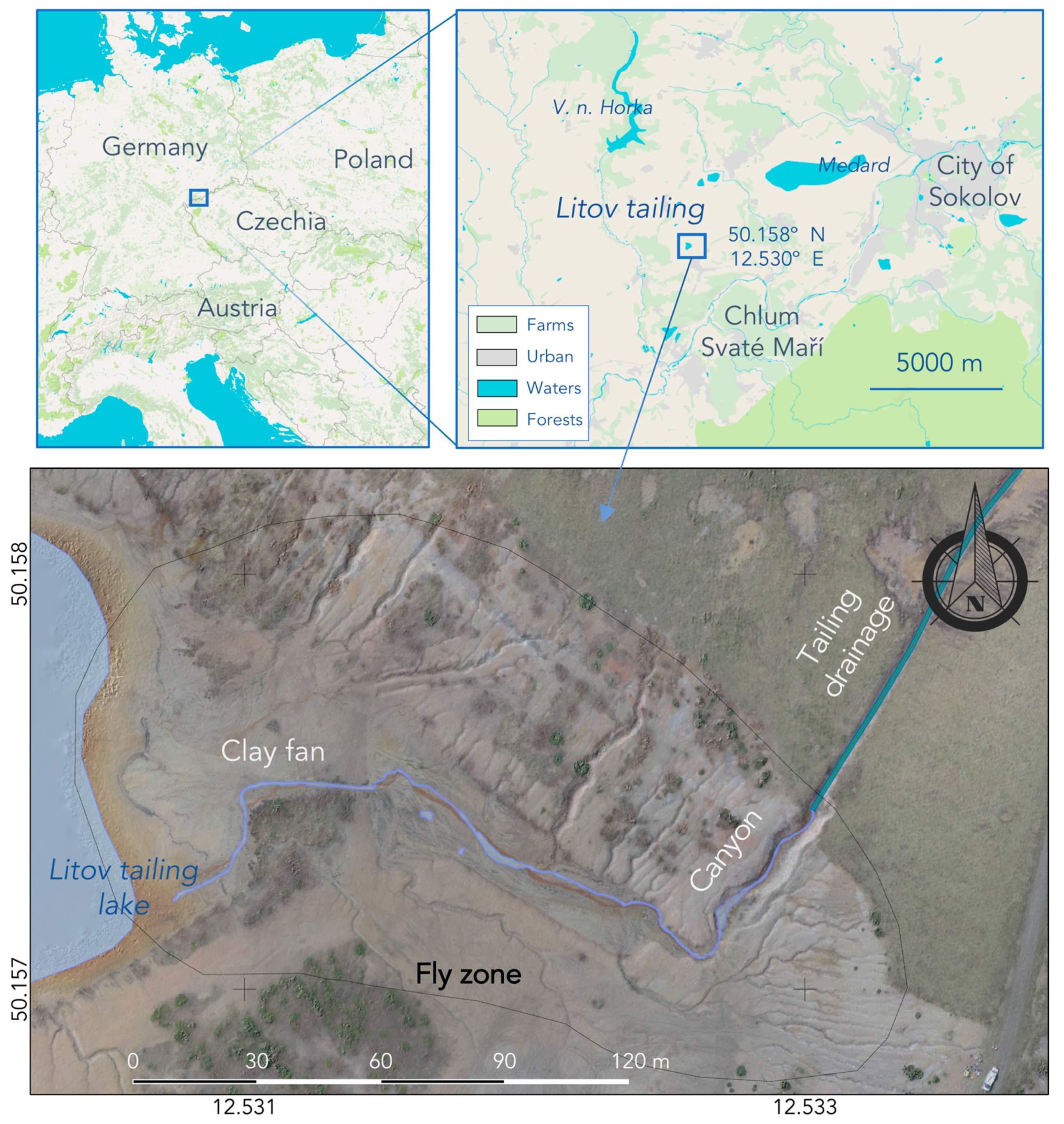
2. Study Area
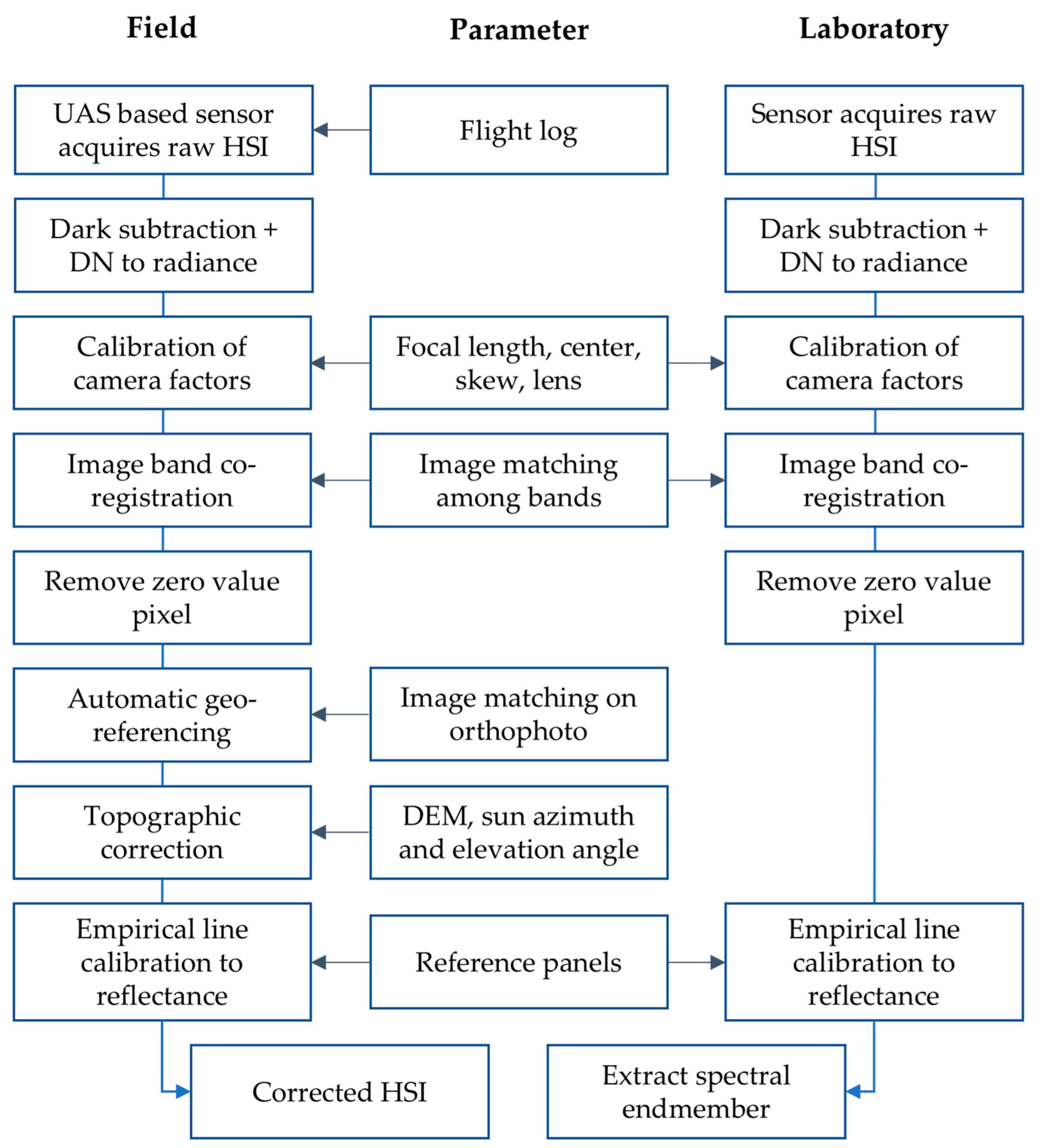
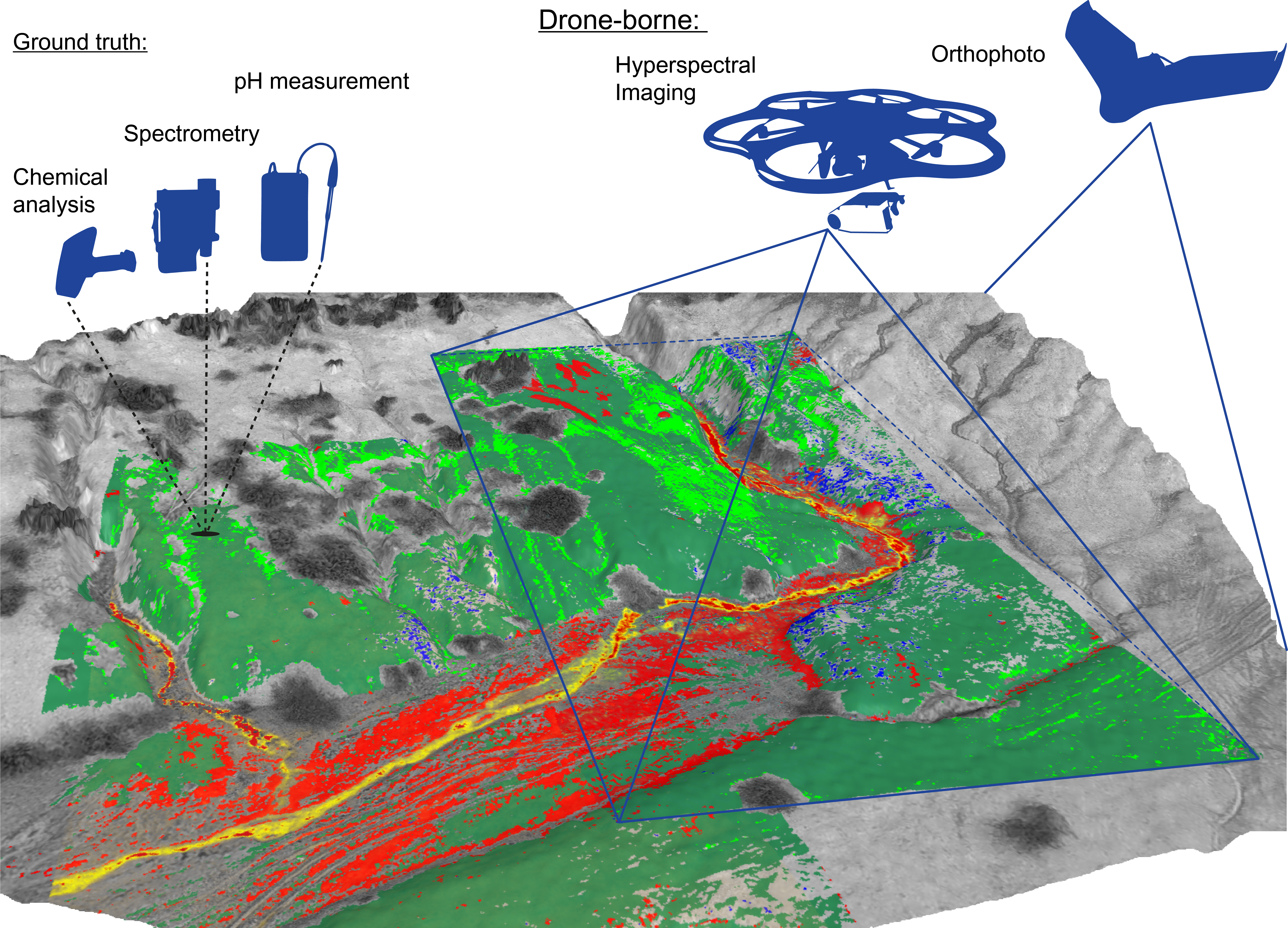
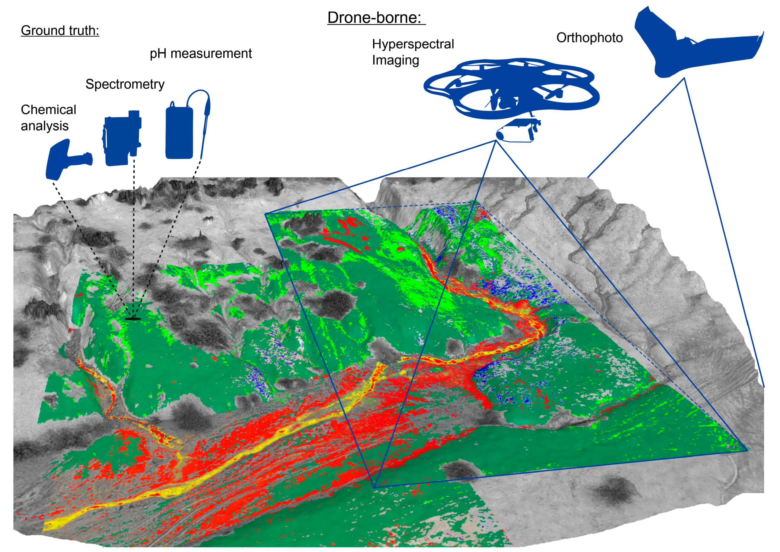
3. Data and Methods
3.1. Hyperspectral Camera and UAS Setup
3.2. UAS Settings
3.3. Laboratory Spectroscopy
3.4. pH Measurements
3.5. Band Ratios and Classifications
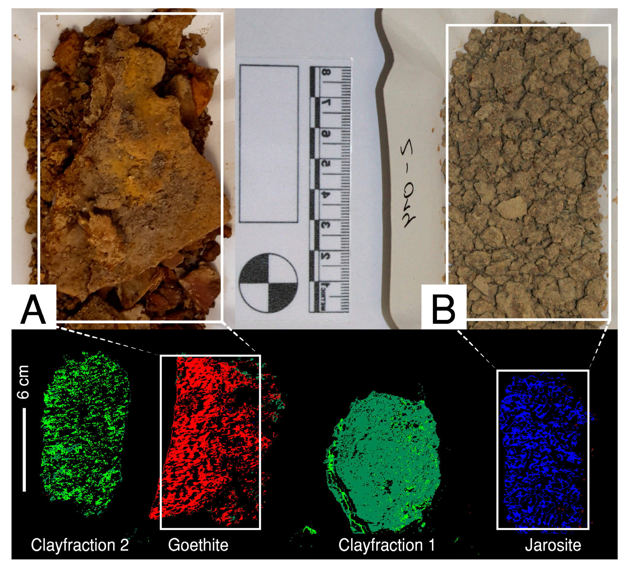
3.6. Mineralogical and Geochemical Sample Evaluation
3.7. Defining the Spectral Endmembers
- 1
- Select fitting samples, visible in at least one HSI with pH value between 2 and 5;
- 2
- Samples typify one characteristic surface feature, e.g., an iron-rich hardpan;
- 3
- Obtain XRF or XRD values and a continuous spectrum from 350–2500 nm, 1024 bands;
- 4
- Scan samples in the laboratory with the Rikola camera from 504–900 nm, 50–80 bands, 20 ms integration time;
- 5
- Extract surface spectrum of characterized samples via unsupervised classifications, e.g., k-means [37];
- 6
- Create the endmember spectral library with all samples, hand spectra, and library spectra for classifications.
4. Results
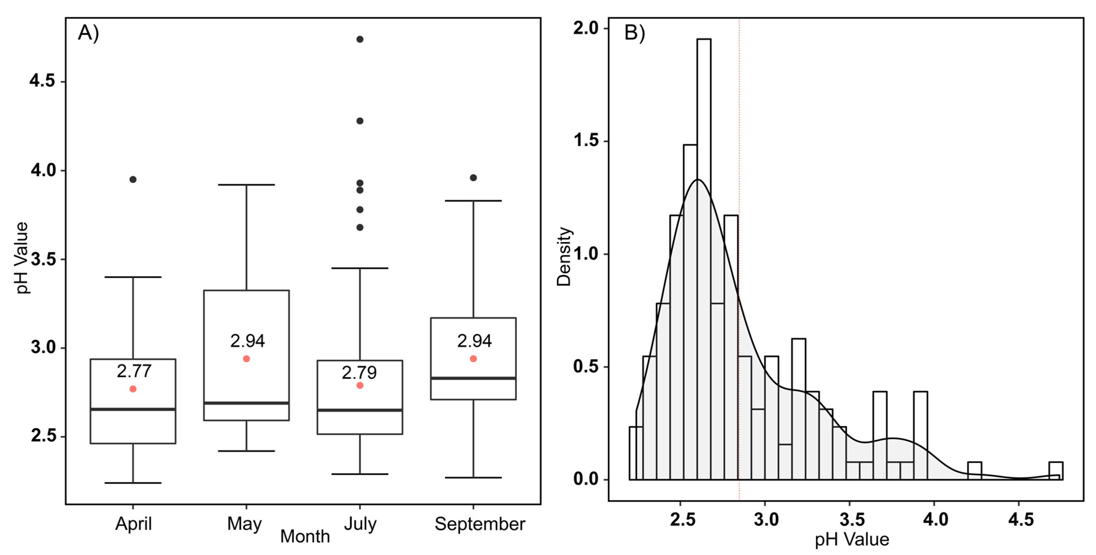
4.1. pH Characterization
4.2. Results of Mineralogical and Geochemical Analyses
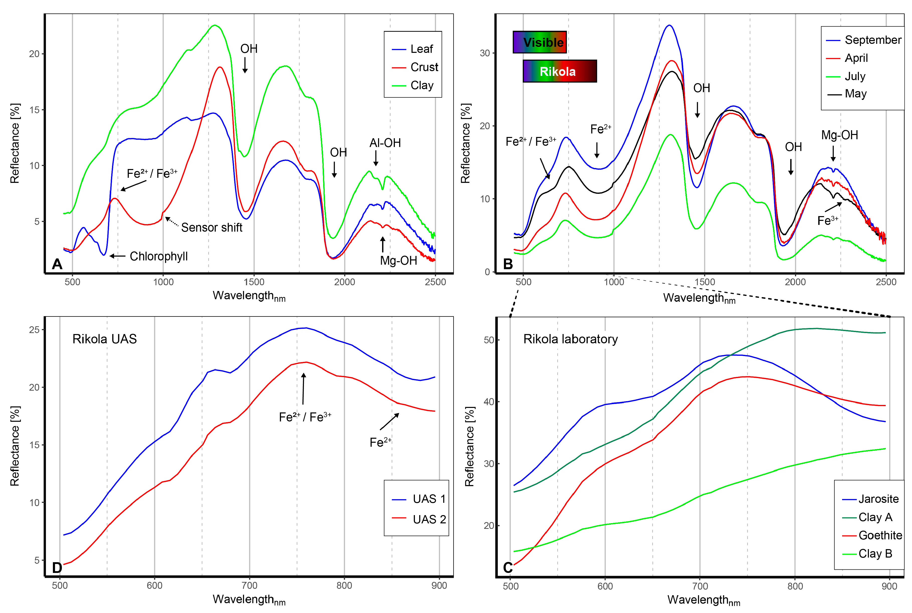
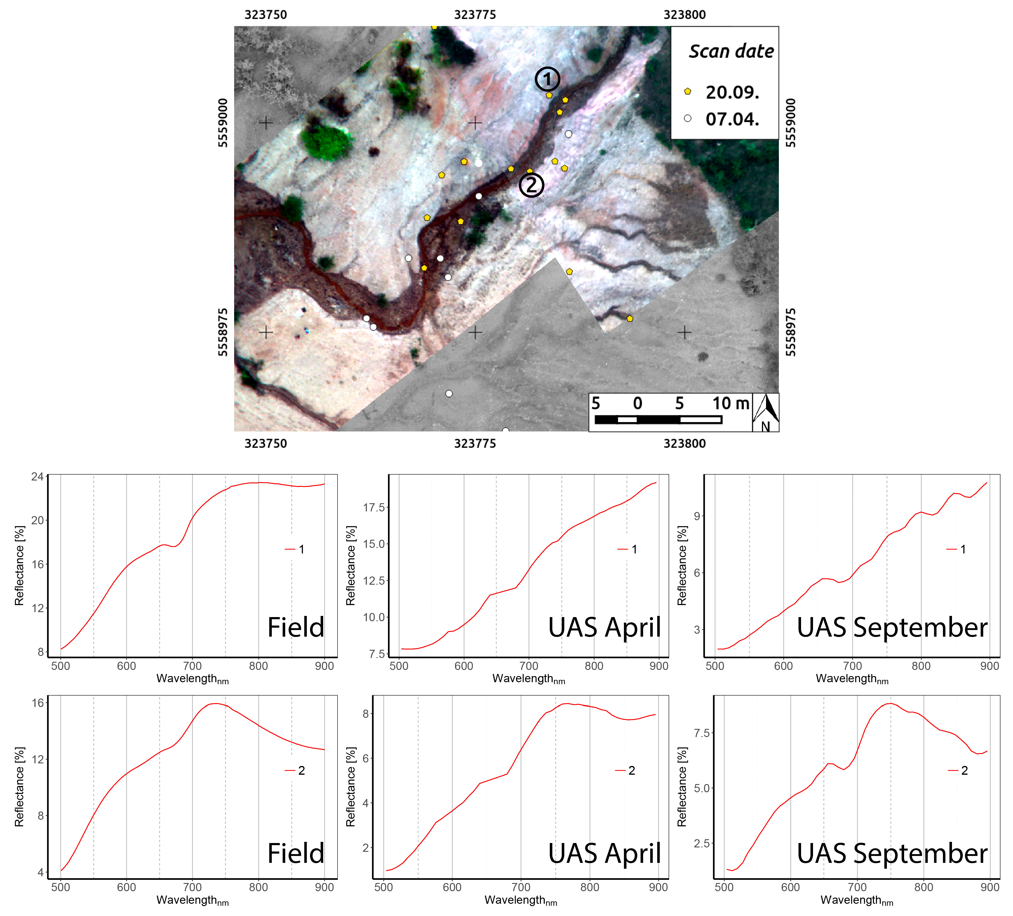
4.3. Field and UAS Spectra Combination, Resulting in the Endmember Selection
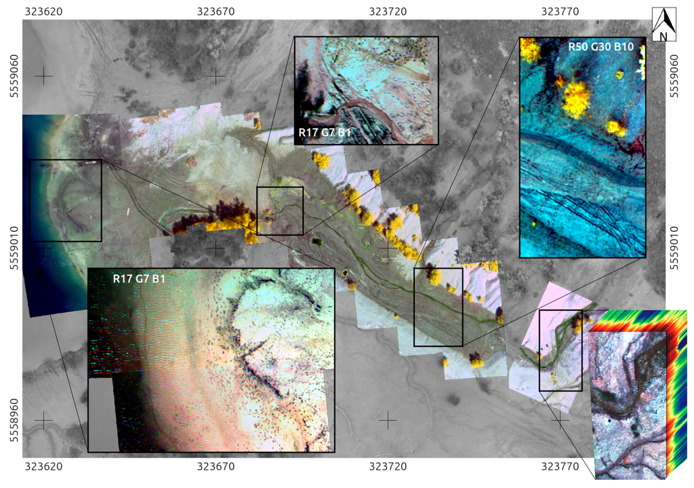
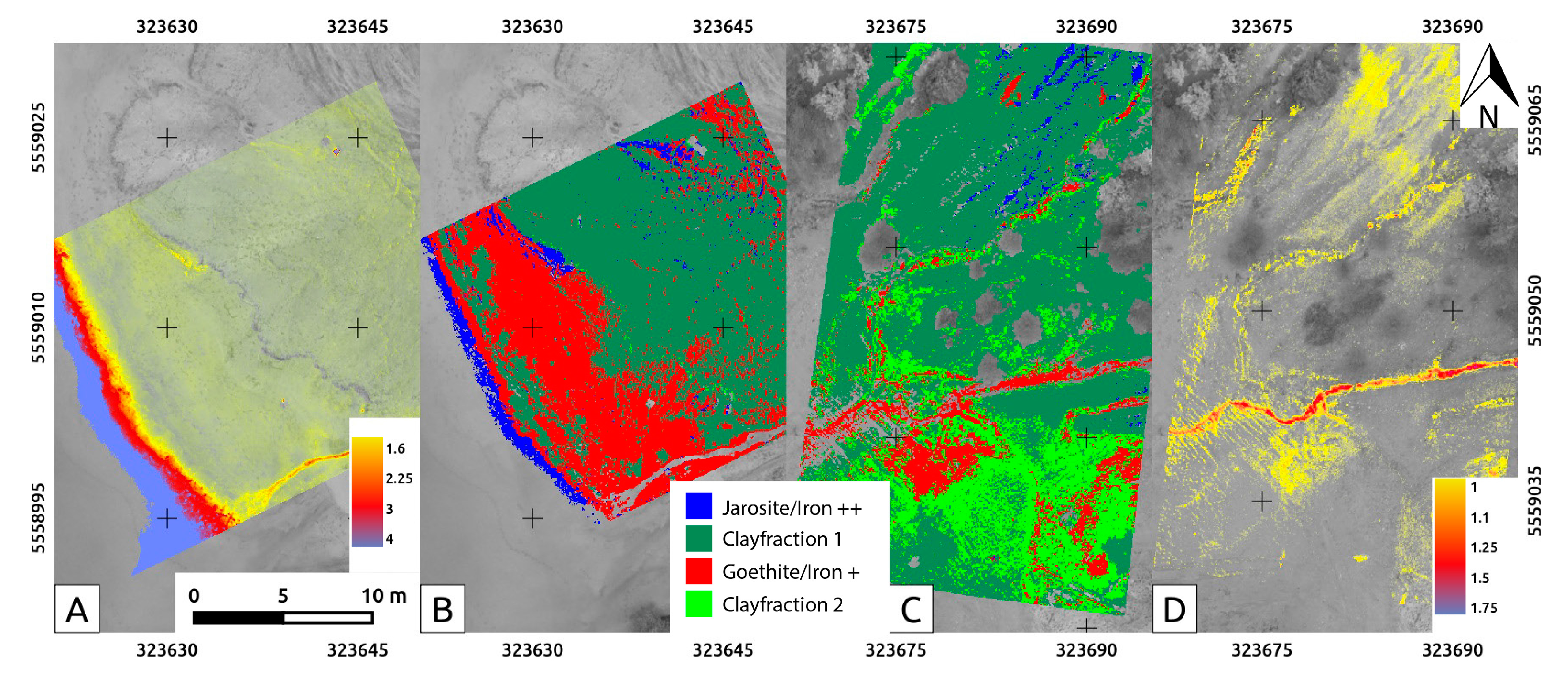
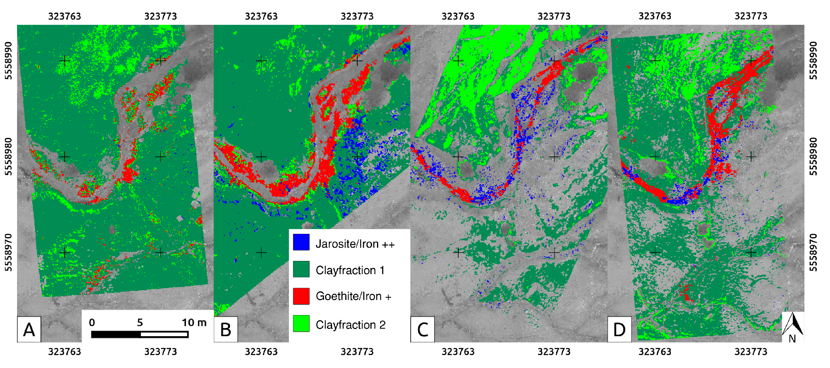
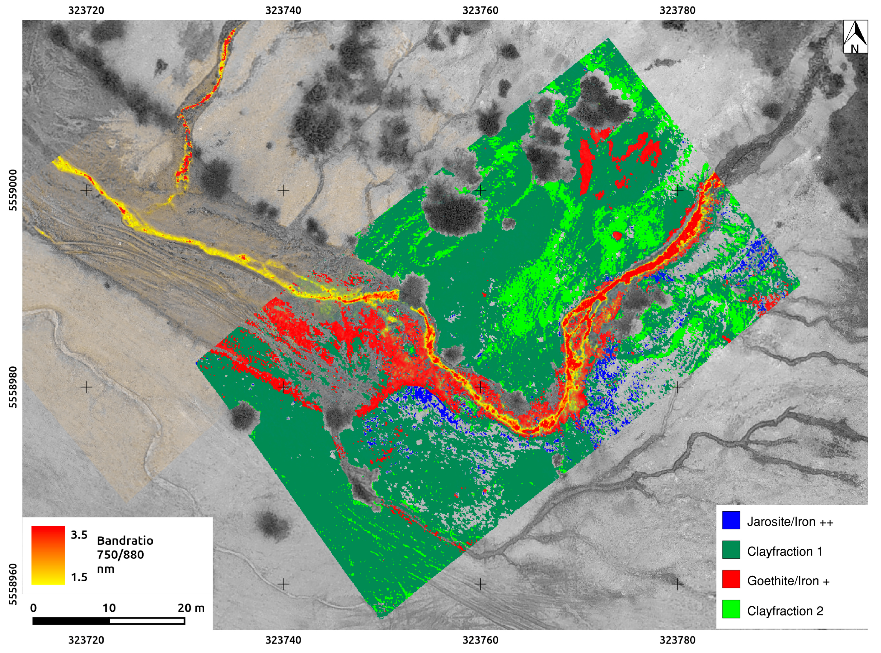
4.4. The Rikola HSIs, Processed and Classified
4.5. Comparing the Spectral Classifications of UAS-Borne HSI
4.6. Rikola Image Spectra
5. Discussion
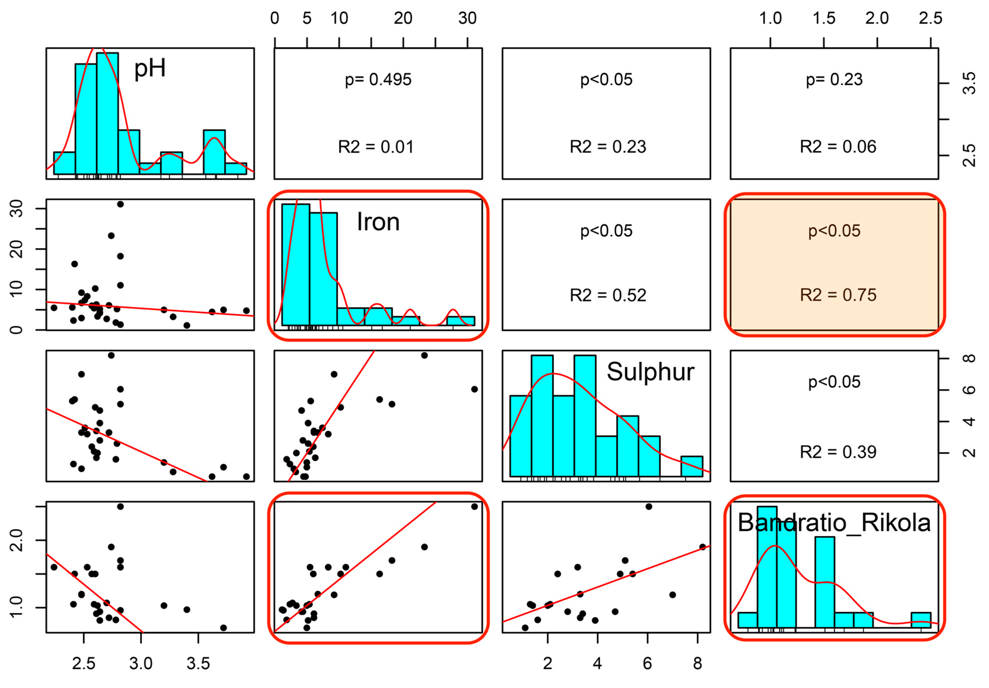
5.1. Evaluation and Relation of pH, Iron, and HSI
5.2. Evaluation of Spectral Classification Results
5.3. Image Quality Evaluation
5.4. Sampling Results
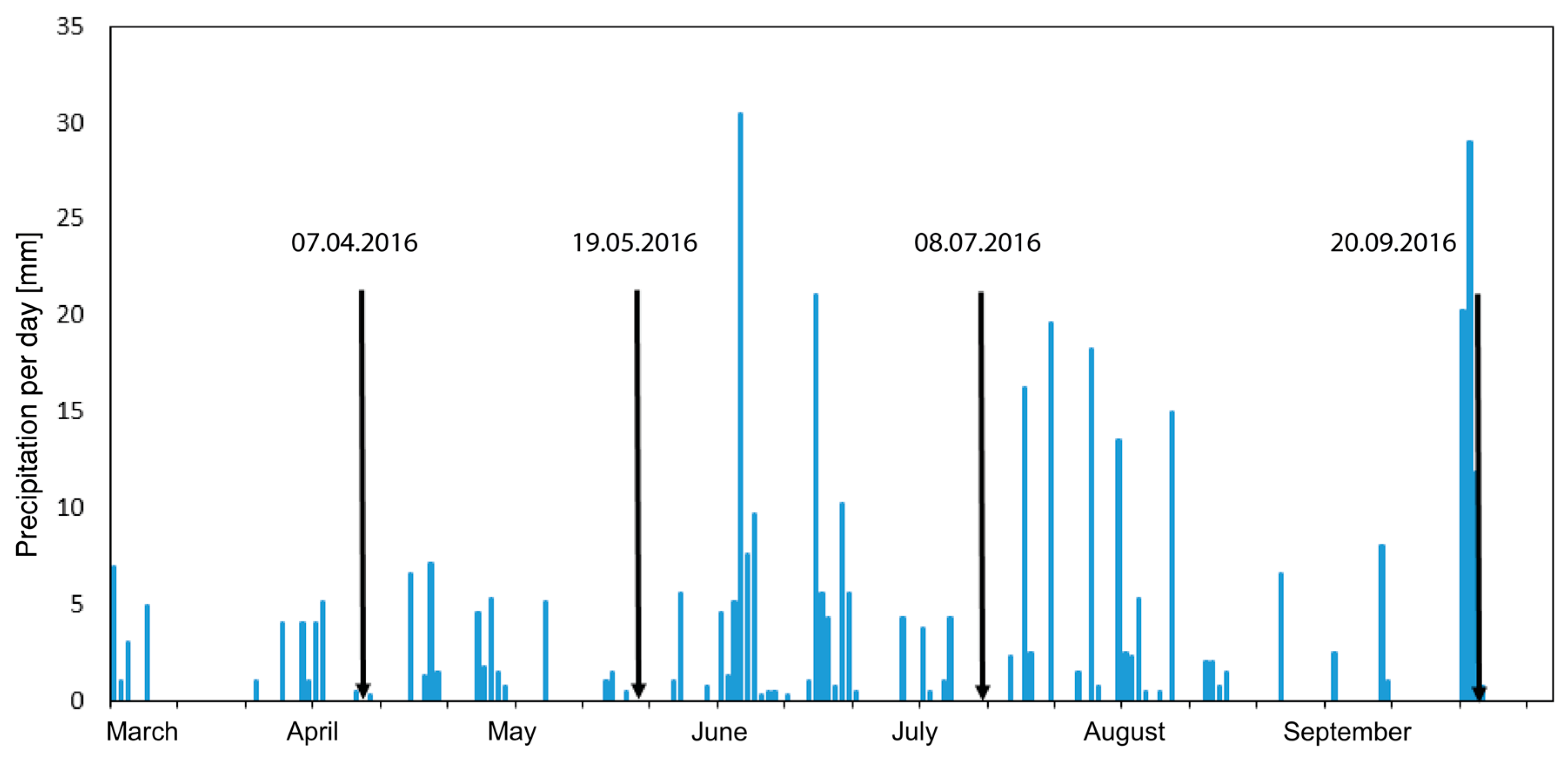
5.5. The Influence of Regional Precipitation
5.6. The Gap between Satellite, Airborne and Drone-Borne Data
6. Conclusions
Acknowledgments
Author Contributions
Conflicts of Interest
References
- Swayze, G.A.; Smith, K.S.; Clark, R.N.; Sutley, S.J.; Pearson, R.M.; Vance, J.S.; Hageman, P.L.; Briggs, P.H.; Meier, A.L.; Singleton, M.J.; et al. Using Imaging Spectroscopy to Map Acidic Mine Waste. Environ. Sci. Technol. 2000, 34, 47–54. [Google Scholar] [CrossRef]
- Wolkersdorfer, C.; Younger, P.L.; Bowell, R. PADRE—Europäische Partnerschaft Für Die Sanierung Saurer Grubenwässer (Partnership for Acid Drainage Remediation in Europe). Wiss. Mitt. 2006, 31, 213–217. [Google Scholar]
- Lottermoser, B.G. Mine Wastes: Characterization, Treatment and Environmental Impacts; Springer-Verlag: Berlin/Heidelberg, Germany, 2010. [Google Scholar]
- Mielke, C.; Boesche, N.K.; Rogass, C.; Kaufmann, H.; Gauert, C.; de Wit, M. Spaceborne Mine Waste Mineralogy Monitoring in South Africa, Applications for Modern Push-Broom Missions: Hyperion/OLI and EnMAP/Sentinel-2. Remote Sens. 2014, 6, 6790–6816. [Google Scholar] [CrossRef]
- Kruse, F.A.; Boardman, J.W.; Huntington, J.F. Comparison of Airborne Hyperspectral Data and EO-1 Hyperion for Mineral Mapping. IEEE Trans. Geosci. Remote Sens. 2003, 41, 1388–1400. [Google Scholar] [CrossRef]
- Zabcic, N.; Rivard, B.; Ong, C.; Miiller, A.; Exploration, C.; Avenue, D.P. Using Airborne Hyperspectral Data to Characterize the Surface pH of Pyrite Mine Tailings. In Proceedings of the Hyperspectral Image and Signal Processing: Evolution in Remote Sensing, Grenoble, France, 26–28 August 2009; IEEE: Piscataway, NJ, USA, 2009; pp. 4–7. [Google Scholar]
- Riaza, A.; Buzzi, J.; García-Meléndez, E.; Carrère, V.; Müller, A. Monitoring the Extent of Contamination from Acid Mine Drainage in the Iberian Pyrite Belt (SW Spain) Using Hyperspectral Imagery. Remote Sens. 2011, 3, 2166–2186. [Google Scholar] [CrossRef]
- Crowley, J.K.; Williams, D.E.; Hammarstrom, J.M.; Piatak, N.; Chou, I.-M.; Mars, J.C. Spectral Reflectance Properties (0.4–2.5 Μm) of Secondary Fe-Oxide, Fe-Hydroxide, and Fe-Sulphate-Hydrate Minerals Associated with Sulphide-Bearing Mine Wastes. Geochem. Explor. Environ. Anal. 2003, 3, 219–228. [Google Scholar] [CrossRef]
- Choe, E.; van der Meer, F.; van Ruitenbeek, F.; van der Werff, H.; de Smeth, B.; Kim, K.W. Mapping of Heavy Metal Pollution in Stream Sediments Using Combined Geochemistry, Field Spectroscopy, and Hyperspectral Remote Sensing: A Case Study of the Rodalquilar Mining Area, SE Spain. Remote Sens. Environ. 2008, 112, 3222–3233. [Google Scholar] [CrossRef]
- Montero, S.I.C.; Brimhall, G.H.; Alpers, C.N.; Swayze, G.A. Characterization of Waste Rock Associated with Acid Drainage at the Penn Mine, California, by Ground-Based Visible to Short-Wave Infrared Reflectance Spectroscopy Assisted by Digital Mapping. Chem. Geol. 2005, 215, 453–472. [Google Scholar] [CrossRef]
- Honkavaara, E.; Eskelinen, M.A.; Polonen, I.; Saari, H.; Ojanen, H.; Mannila, R.; Holmlund, C.; Hakala, T.; Litkey, P.; Rosnell, T.; et al. Remote Sensing of 3-D Geometry and Surface Moisture of a Peat Production Area Using Hyperspectral Frame Cameras in Visible to Short-Wave Infrared Spectral Ranges Onboard a Small Unmanned Airborne Vehicle (UAV). IEEE Trans. Geosci. Remote Sens. 2016, 54, 5440–5454. [Google Scholar] [CrossRef]
- Aasen, H.; Burkart, A.; Bolten, A.; Bareth, G. Generating 3D Hyperspectral Information with Lightweight UAV Snapshot Cameras for Vegetation Monitoring: From Camera Calibration to Quality Assurance. ISPRS J. Photogramm. Remote Sens. 2015, 108, 245–259. [Google Scholar] [CrossRef]
- Roosjen, P.P.J.; Suomalainen, J.M.; Bartholomeus, H.M.; Clevers, J.G.P.W. Hyperspectral Reflectance Anisotropy Measurements Using a Pushbroom Spectrometer on an Unmanned Aerial Vehicle-Results for Barley, Winter Wheat, and Potato. Remote Sens. 2016, 8, 909. [Google Scholar] [CrossRef]
- Jakob, S.; Zimmermann, R.; Gloaguen, R. The Need for Accurate Geometric and Radiometric Corrections of Drone-Borne Hyperspectral Data for Mineral Exploration: MEPHySTo-A Toolbox for Pre-Processing Drone-Borne Hyperspectral Data. Remote Sens. 2017, 9, 88. [Google Scholar] [CrossRef]
- Colomina, I.; Molina, P. Unmanned Aerial Systems for Photogrammetry and Remote Sensing: A Review. ISPRS J. Photogramm. Remote Sens. 2014, 92, 79–97. [Google Scholar] [CrossRef]
- Hruska, R.; Mitchell, J.; Anderson, M.; Glenn, N.F. Radiometric and Geometric Analysis of Hyperspectral Imagery Acquired from an Unmanned Aerial Vehicle. Remote Sens. 2012, 4, 2736–2752. [Google Scholar] [CrossRef]
- Murfitt, S.L.; Allan, B.M.; Bellgrove, A.; Rattray, A.; Young, M.A.; Ierodiaconou, D. Applications of Unmanned Aerial Vehicles in Intertidal Reef Monitoring. Sci. Rep. 2017, 7, 1–11. [Google Scholar] [CrossRef] [PubMed]
- Jaud, M.; Le Dantec, N.; Ammann, J.; Grandjean, P.; Constantin, D.; Akhtman, Y.; Barbieux, K.; Allemand, P.; Delacourt, C.; Merminod, B. Direct Georeferencing of a Pushbroom, Lightweight Hyperspectral System for Mini-UAV Applications. Remote Sens. 2018, 10, 204. [Google Scholar] [CrossRef]
- Adão, T.; Hruška, J.; Pádua, L.; Bessa, J.; Peres, E.; Morais, R.; Sousa, J.J. Hyperspectral Imaging: A Review on UAV-Based Sensors, Data Processing and Applications for Agriculture and Forestry. Remote Sens. 2017, 9, 1110. [Google Scholar] [CrossRef]
- Adar, S.; Notesco, G.; Brook, A.; Livne, I.; Rojik, P.; Kopačková, V.; Zelenkova, K.; Misurec, J.; Bourguignon, A.; Chevrel, S.; et al. Change Detection over Sokolov Open-Pit Mining Area, Czech Republic, Using Multi-Temporal HyMAP Data (2009–2010). SPIE Remote Sens. 2011, 8180, 9. [Google Scholar]
- Kopačková, V. Using Multiple Spectral Feature Analysis for Quantitative pH Mapping in a Mining Environment. Int. J. Appl. Earth Obs. Geoinf. 2014, 28, 28–42. [Google Scholar] [CrossRef]
- Kopačková, V.; Chevrel, S.; Bourguignon, A.; Rojík, P. Application of High Altitude and Ground-Based Spectroradiometry to Mapping Hazardous Low-pH Material Derived from the Sokolov Open-Pit Mine. J. Maps 2012, 8, 220–230. [Google Scholar] [CrossRef]
- Murad, E.; Rojík, P. Jarosite, schwertmannite, goethite ferrihydrite and lepidocrocite: the legacy of coal and sulfide ore mining. SuperSoil 2004, 3, 5–9. [Google Scholar]
- Kopačková, V.; Hladíková, L. Applying Spectral Unmixing to Determine Surface Water Parameters in a Mining Environment. Remote Sens. 2014, 6, 11204–11224. [Google Scholar] [CrossRef]
- Bigham, J.M.; Schwertmann, U.; Pfab, G. Influence of pH on Mineral Speciation in a Bioreactor Simulating Acid Mine Drainage. Appl. Geochem. 1996, 11, 845–849. [Google Scholar] [CrossRef]
- Hunt, G.R.; Ashley, R.P. Spectra of Altered Rocks in the Visible and near Infrared. Econ. Geol. 1979, 74, 1613–1629. [Google Scholar] [CrossRef]
- Bishop, J.L.; Murad, E. The Visible and Infrared Spectral Properties of Jarosite and Alunite. Am. Mineral. 2005, 90, 1100–1107. [Google Scholar] [CrossRef]
- Bigham, J.M.; Schwertmann, U.; Traina, S.J.; Winland, R.L.; Wolf, M. Schwertmannite and the Chemical Modeling of Iron in Acid Sulfate Waters. Geochim. Cosmochim. Acta 1996, 60, 2111–2121. [Google Scholar] [CrossRef]
- Davies, G.E.; Calvin, W.M. Quantifizierung Der Eisenkonzentration von Synthetischer Und in Situ Vorkommender Saurer Bergbaudränage: Eine Neue Technik Unter Nutzung Tragbarer Feldspektrometer. Mine Water Environ. 2017, 36, 299–309. [Google Scholar] [CrossRef]
- Jordan, C.J.; Chevrel, S.; Coetzee, H.; Ben-Dor, E.; Ehrler, C.; Fischer, C.; Grebby, S.R.; Kerr, G.; Livne, I.; Kopačková, V.; et al. EO-MINERS: Monitoring the Environmental and Societal Impact of the Extractive Industry Using Earth Observation. In Proceedings of the 2013 IEEE International Geoscience and Remote Sensing Symposium (IGARSS), Melbourne, VIC, Australia, 21–26 July 2013; 1741–1744. [Google Scholar]
- Denk, M.; Glaesser, C.; Kurz, T.H.; Buckley, S.J.; Drissen, P. Mapping of Iron and Steelwork by-Products Using Close Range Hyperspectral Imaging: A Case Study in Thuringia, Germany. Eur. J. Remote Sens. 2015, 48, 489–509. [Google Scholar] [CrossRef]
- Ziegler, P.A. European Cenozoic Rift System. Tectonophysics 1992, 208, 91–111. [Google Scholar] [CrossRef]
- Rojík, P. New Stratigraphic Subdivision of the Tertiary in the Sokolov Basin in Northwestern Bohemia. J. Czech Geol. Soc. 2004, 49, 173–185. [Google Scholar]
- Murad, E.; Rojík, P. Iron Mineralogy of Mine-Drainage Precipitates as Environmental Indicators: Review of Current Concepts and a Case Study from the Sokolov Basin, Czech Republic. Clay Miner. 2005, 40, 427–440. [Google Scholar] [CrossRef]
- Kupková, L.; Potucková, M.; Zachová, K.; Lhtáková, Z.; Kopačková, V.; Albrechtová, J. Chlorophyll Determination in Silver Birch and Scots Pine Foliage from Heavy Metal Polluted Regions Using Spectral Reflectance Data. EARSeL eProc. 2012, 11, 64–73. [Google Scholar]
- Van der Meer, F.D.; van der Werff, H.M.A.; van Ruitenbeek, F.J.A.; Hecker, C.A.; Bakker, W.H.; Noomen, M.F.; van der Meijde, M.; Carranza, E.J.M.; de Smeth, J.B.; Woldai, T. Multi- and Hyperspectral Geologic Remote Sensing: A Review. Int. J. Appl. Earth Obs. Geoinf. 2012, 14, 112–128. [Google Scholar] [CrossRef]
- Makelainen, A.; Saari, H.; Hippi, I.; Sarkeala, J.; Soukkamaki, J. 2D Hyperspectral Frame Imager Camera Data in Photogrammetric Mosaicking. Int. Arch. Photogramm. Remote Sens. Spat. Inf. Sci. 2013, XL-1/W2, 263–267. [Google Scholar] [CrossRef]
- Savitzky, A.; Golay, M.J.E. Smoothing and Differentiation of Data by Simplified Least Squares Procedures. Anal. Chem. 1964, 36, 1627–1639. [Google Scholar] [CrossRef]
- Spectralon Technical Datashet-Reflectance Materials and Coatings; Technical guide; Labsphere: North Sutton, NH, USA, 2016; pp. 1–26.
- PhotoScan Professional Version 1.2.5; Agisoft LLC: St. Petersburg, Russia, 2016.
- Soil Quality—Determination of pH 10390:2005. 13.080.10—Chemical characteristics of soils; DIN-ISO Technical Committee ISO/TC 190-SC 3: Bad Mergentheim, Germany, 2005.
- Tucker, C.J. Red and Photographic Infrared Linear Combinations for Monitoring Vegetation. Remote Sens. Environ. 1979, 8, 127–150. [Google Scholar] [CrossRef]
- Kruse, F.A.; Lefkoff, A.B.; Boardman, J.W.; Heidebrecht, K.B.; Shapiro, A.T.; Barloon, P.J.; Goetz, A.F.H. The Spectral Image Processing System (SIPS)—Interactive Visualization and Analysis of Imaging Spectrometer Data. Remote Sens. Environ. 1993, 44, 145–163. [Google Scholar] [CrossRef]
- Younger, P.L.; Banwart, S.; Hedin, R.S. Mine Water: Hydrology, Pollution, Remediation; Springer: Dordrecht, The Netherlands, 2002; Volume 53. [Google Scholar]
- S1 Titan Model 600/800 GeoChem Data Sheet; Bruker: Berlin, Germany, 2014.
- Brammer Standards Geological Materials Catalogue; Brammer Standard Company Inc.: Houston, Texas, USA, 2014.
- Clark, R.N.; Swayze, G.A.; Wise, R.; Livo, E.; Hoefen, T.; Kokaly, R.; Sutley, S.J. USGS Digital Spectral Library Splib06a; U.S. Geological Survey: Reston, VA, USA, 2007.
- Hubbard, B.E.; Crowley, J.K.; Zimbelman, D.R. Hyperion, ALI, and ASTER Imagery. Comp. Gen. Pharmacol. 2003, 41, 1401–1410. [Google Scholar]
- Aldrich, J. Correlations Genuine and Spurious in Pearson and Yule. Stat. Sci. 1995, 10, 364–376. [Google Scholar] [CrossRef]


| Mineral | Formula | Spectral Feature Position [nm] |
|---|---|---|
| Jarosite | 436 a, 716 p, 920 a, 1465 a 2264 a | |
| Schwertmannite | 545 e, 738 p, 912 a 1449 a, 1945 a | |
| Goethite | 484 e, 668 e, 760 p, 932 a, 1454 a, 1944 a | |
| Hematite | 586 e, 744 p, 868 a |
| Parameter | Value |
|---|---|
| FOV | 36.5° |
| Spectral range | 504–900 nm |
| Spectral resolution | ~10 nm, FWHM |
| Spectral bands | 50 D, 80 L |
| Integration time per band | 10–50 ms, depends on light conditions |
| Pixel resolution | 1010 × 624 D, 1010 × 1010 L |
| Weight | 720 g |
| Parameter | Aibot X6 V2 Hexacopter | eBee Fixed Wing |
|---|---|---|
| Camera system | Rikola | Canon Powershot S110 RGB |
| Flight duration | 8–15 min | 15–25 min |
| Weight | 5 kg | 700 g |
| Altitude | 50 m | 120 m |
| Area covered per flight | 6000–10,000 m2 | 0.6 km2 |
| Shutter time | 10–25 ms | 10–50 ms, depending on light |
| Resolution on ground | 3–5 cm | 5–15 cm |
| Sensor resolution | 1010 × 624 Pix | 12 MPix |
| April: F/I | 3/20 ** | 1/227 |
| May: F/I | 2/34 | 1 */104 |
| July: F/I | 1/23 | 1/125 |
| September: F/I | 2/41 | 1/204 |
| 2-010 | wt % | 2-014 | wt % | 2-022 | wt % | 3-007 | wt % | 3-077 | wt % |
|---|---|---|---|---|---|---|---|---|---|
| Kaolinite | 55.8 | Kaolinite | 39.2 | Kaolinite | 59.8 | Kaolinite | 65.5 | Kaolinite | 48.7 |
| Quartz | 23.5 | Quartz | 26.6 | Quartz | 17.3 | Quartz | 17.5 | Quartz | 24.1 |
| Jarosite | 7.6 | Jarosite | 21.7 | Jarosite | 7.5 | Jarosite | 7.0 | Jarosite | 4.9 |
| Goethite | 2.5 | Goethite | 7.0 | Goethite | 2.8 | Cristobalite | 5.6 | Goethite | 11.1 |
| Muscovite | 5.0 | Gypsum | 2.1 | Muscovite | 7.7 | Gypsum | 3.1 | Cristobalite | 4.5 |
| Anatase | 1.9 | Titanite | 1.4 | Crisobalite | 1.5 | Anatase | 1.5 | Muscovite | 4.3 |
| Gypsum | 1.7 | Muscovite | 1.3 | Gypsum | 1.5 | Rutile | 0.7 | Rutile | 1.0 |
| Cristobalite | 1.4 | Anatase | 0.6 | Anatase | 1.4 | Gypsum | 0.7 | ||
| Titanite | 0.5 |
© 2018 by the authors. Licensee MDPI, Basel, Switzerland. This article is an open access article distributed under the terms and conditions of the Creative Commons Attribution (CC BY) license (http://creativecommons.org/licenses/by/4.0/).
Share and Cite
Jackisch, R.; Lorenz, S.; Zimmermann, R.; Möckel, R.; Gloaguen, R. Drone-Borne Hyperspectral Monitoring of Acid Mine Drainage: An Example from the Sokolov Lignite District. Remote Sens. 2018, 10, 385. https://doi.org/10.3390/rs10030385
Jackisch R, Lorenz S, Zimmermann R, Möckel R, Gloaguen R. Drone-Borne Hyperspectral Monitoring of Acid Mine Drainage: An Example from the Sokolov Lignite District. Remote Sensing. 2018; 10(3):385. https://doi.org/10.3390/rs10030385
Chicago/Turabian StyleJackisch, Robert, Sandra Lorenz, Robert Zimmermann, Robert Möckel, and Richard Gloaguen. 2018. "Drone-Borne Hyperspectral Monitoring of Acid Mine Drainage: An Example from the Sokolov Lignite District" Remote Sensing 10, no. 3: 385. https://doi.org/10.3390/rs10030385
APA StyleJackisch, R., Lorenz, S., Zimmermann, R., Möckel, R., & Gloaguen, R. (2018). Drone-Borne Hyperspectral Monitoring of Acid Mine Drainage: An Example from the Sokolov Lignite District. Remote Sensing, 10(3), 385. https://doi.org/10.3390/rs10030385