Comparison of Three Methods for Estimating GPS Multipath Repeat Time


Abstract
:
1. Introduction
2. Methods
2.1. Orbit Repeat Time Method (ORTM)
2.2. Aspect Repeat Time Adjustment (ARTA)
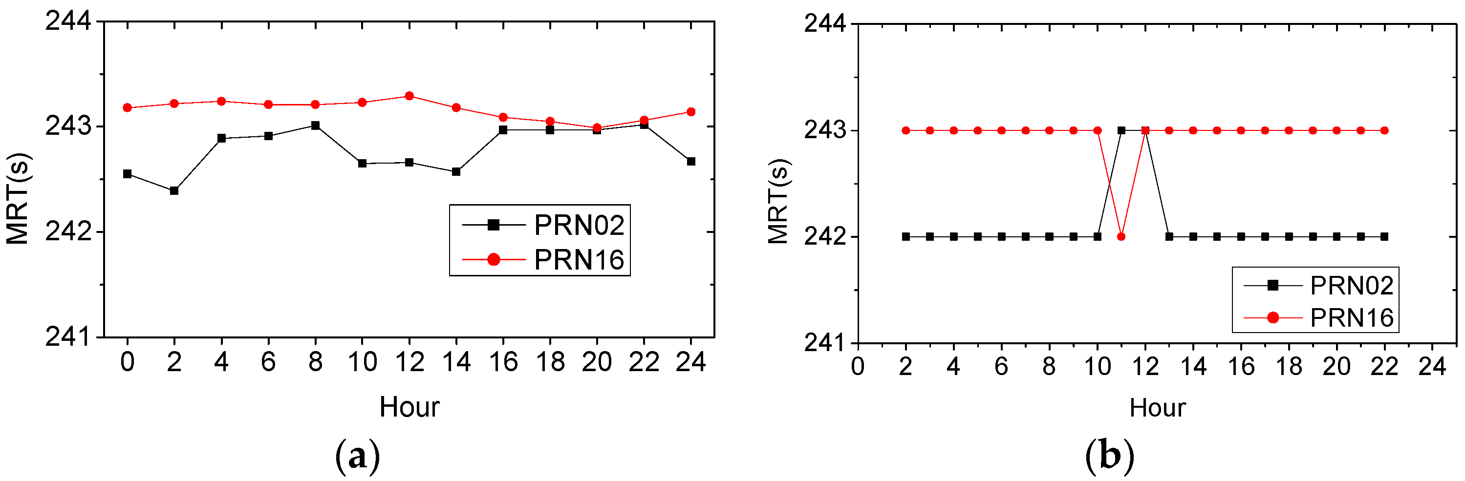
2.3. Residual Correlation Method (RCM)
3. Experiment and Results
3.1. ORTM-Derived MRT vs. ARTA-Derived MRT
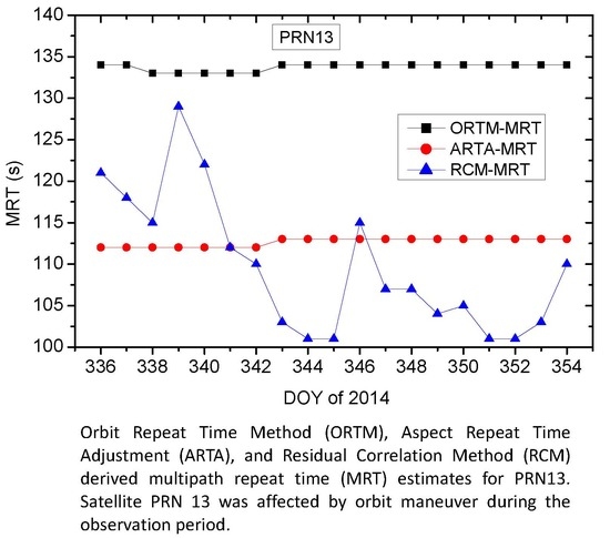
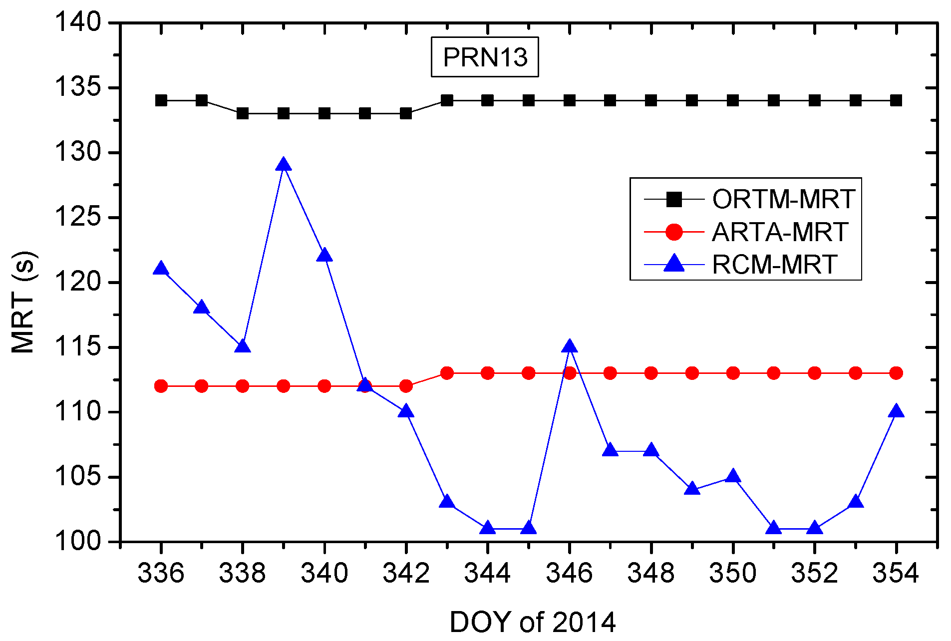
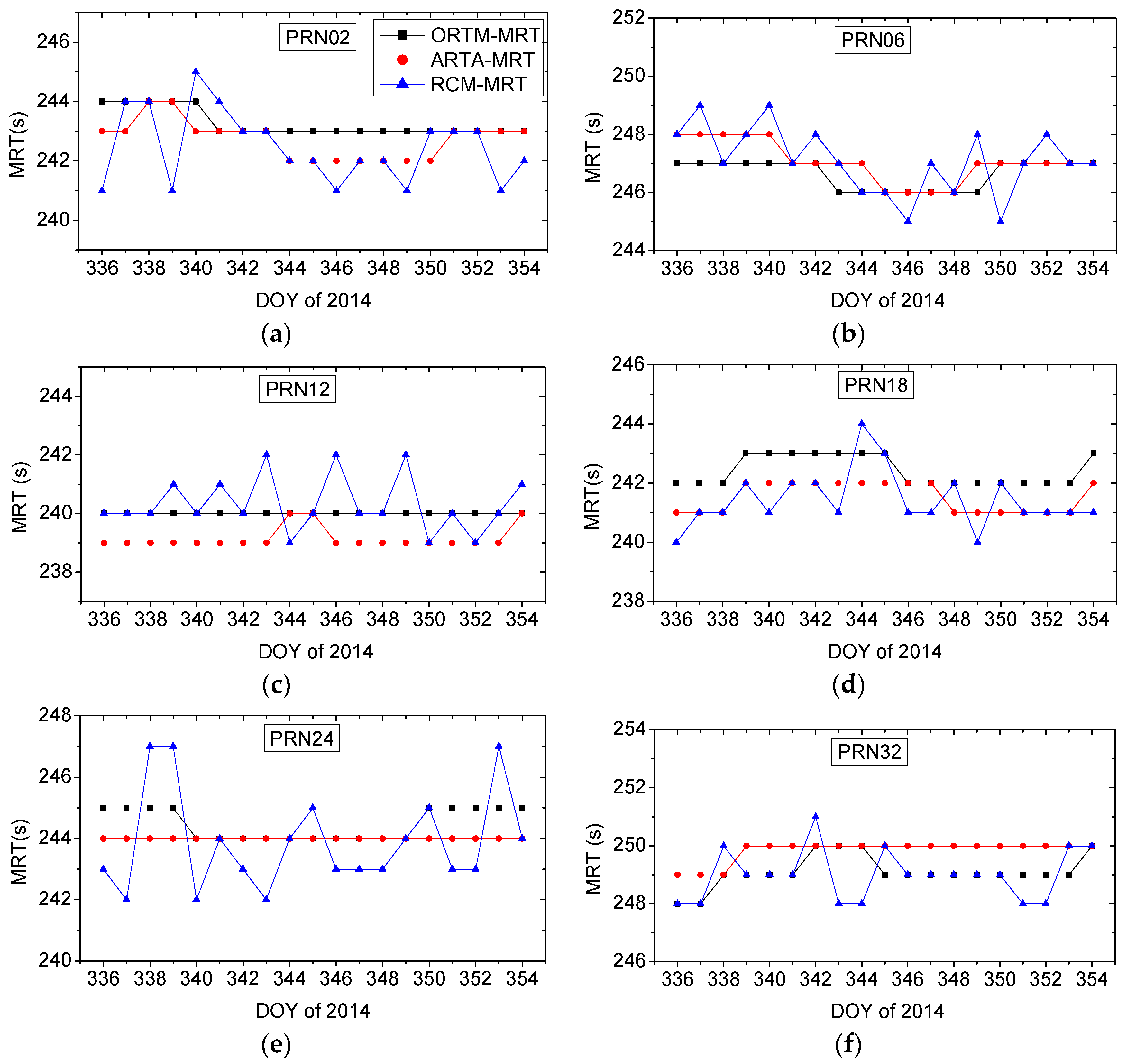
3.2. MRT Derived from the Three Methods
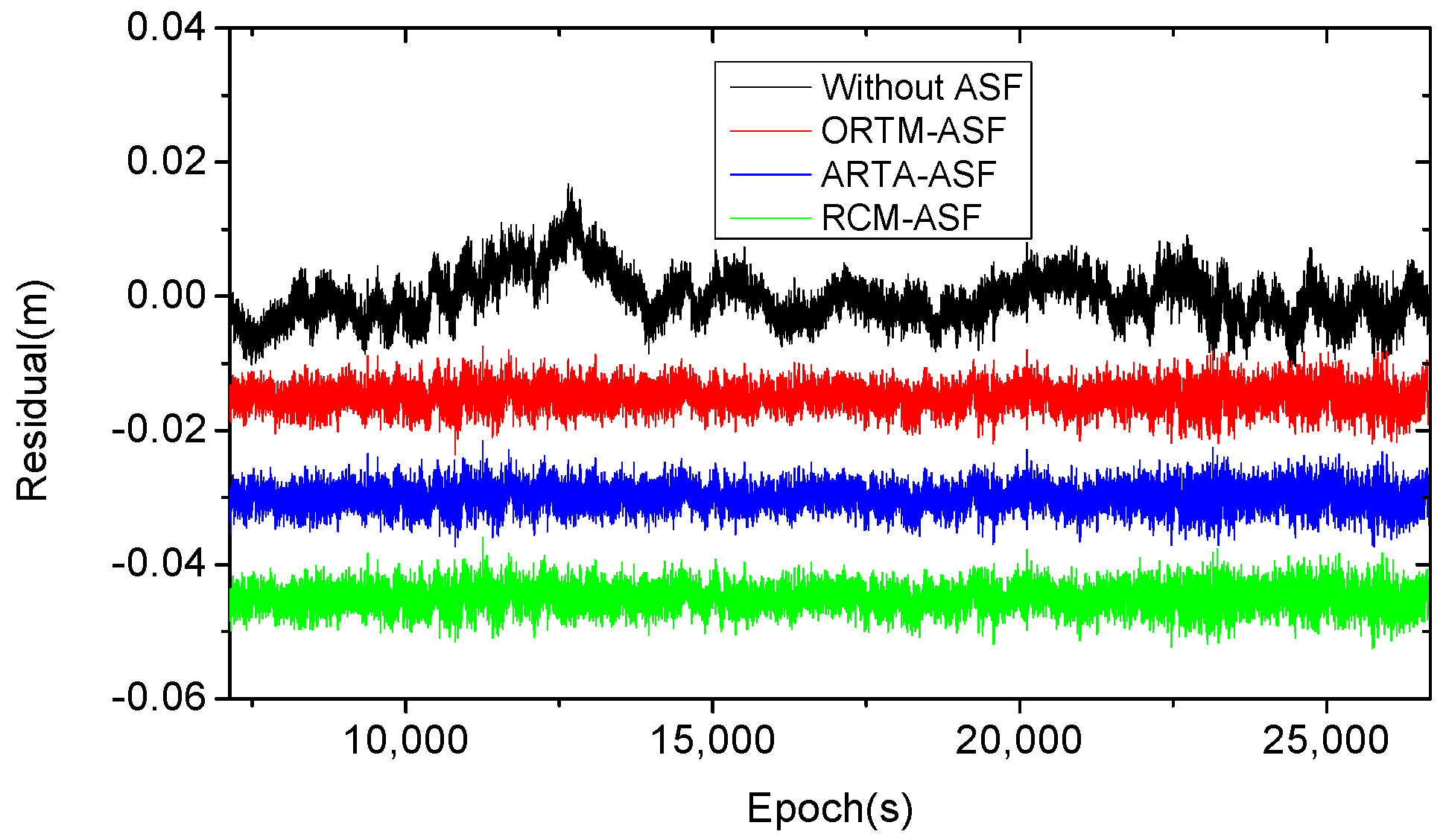
3.3. Effectiveness of Multipath Mitigation
3.4. Robustness, Computational Cost and Real-Time Application
4. Discussion
5. Conclusions
Acknowledgments
Author Contributions
Conflicts of Interest
Abbreviations
| GNSS | Global Navigation Satellite System |
| GPS | Global Positioning System |
| GLONASS | Globalnaya navigatsionnaya sputnikovaya Sistema |
| BDS | BeiDou Navigation Satellite System |
| GALILEO | Galileo Navigation Satellite System |
| MRT | Multipath Repeat Time |
| ORTM | Orbit Repeat Time Method |
| ARTA | Aspect Repeat Time Adjustment |
| RCM | Residual Correlation Method |
| ASF | Advanced Sidereal Filtering |
| DOY | Day of Year |
| N, E, and U | North, East, and Up |
| PRN | Pseudo Random Noise Code Number |
| STD | Standard Deviation |
| RMS | Root Mean Square |
| IGS | International GNSS Service |
| SOPAC | Scripps Orbit and Permanent Array Center |
| CDDIS | Crustal Dynamics Data Information System |
References
- Hofmann-Wellenhof, B.; Lichtenegger, H.; Wasle, E. GNSS—Global Naviagtion Satellite System; Springer: Vienna, Austria, 2008; pp. 154–155. ISBN 978-3-211-73012-6. [Google Scholar]
- Park, K.; Nerem, R.; Schenewerk, M.; Davis, J. Site-specific multipath characteristics of global IGS and CORS GPS sites. J. Geod. 2004, 77, 799–803. [Google Scholar] [CrossRef]
- Bock, Y. Continuous monitoring of crustal deformation. GPS World 1991, 2, 40–47. [Google Scholar]
- Genrich, J.; Bock, Y. Rapid resolution of crustal motion at short ranges with the Global Positioning System. J. Geophys. Res. 1992, 97, 3261–3269. [Google Scholar] [CrossRef]
- Wübbena, G.; Schmitz, M.; Menge, F.; Seeber, G.; Völksen, C. A new approach for field calibration of absolute GPS antenna phase center variations. Navigation 1997, 44, 247–255. [Google Scholar] [CrossRef]
- Choi, K.; Bilich, A.; Larson, K.; Axelrad, P. Modified sidereal filtering: Implications for high-rate GPS positioning. Geophys. Res. Lett. 2004, 31, L22608. [Google Scholar] [CrossRef]
- Yin, H.; Gan, W.; Xiao, G. Modified sidereal filter and its effect on high-rate GPS positioning. Geomat. Inf. Sci. Wuhan Univ. 2011, 36, 609–611. [Google Scholar]
- Larson, K.; Bilich, A.; Axelrad, P. Improving the precision of high-rate GPS. J. Geophys. Res. 2007, 112, B05422. [Google Scholar] [CrossRef]
- Ragheb, A.; Clarke, P.; Edwards, S. GPS sidereal filtering: Coordinate and carrier-phase-level strategies. J. Geod. 2007, 81, 325–335. [Google Scholar] [CrossRef]
- Fang, R. High-Rate GPS Data Non-Difference Precise Processing and Its Application on Seismology. Ph.D. Thesis, Wuhan University, Wuhan, China, 2010. [Google Scholar]
- Zhong, P.; Ding, X.; Yuan, L.; Xu, Y.; Kwok, K.; Chen, Y. Sidereal filtering based on single differences for mitigating GPS multipath effects on short baselines. J. Geod. 2010, 84, 145–158. [Google Scholar] [CrossRef]
- Lau, L. Comparison of measurement and position domain multipath filtering techniques with the repeatable GPS orbits for static antennas. Surv. Rev. 2012, 44, 9–16. [Google Scholar] [CrossRef]
- Atkins, C.; Ziebart, M. Effectiveness of observation-domain sidereal filtering for GPS precise point positioning. GPS Solut. 2016, 20, 111–122. [Google Scholar] [CrossRef]
- Zheng, D.; Zhong, P.; Ding, X.; Chen, W. Filtering GPS time-series using a Vondrak filter and cross validation. J. Geod. 2005, 79, 363–369. [Google Scholar] [CrossRef]
- Shen, F.; Li, J.; Zhang, X.; Shu, C. The improved sidereal filtering of time series considering segments’ similarity in coseismic displacement. Acta Geod. Cartogr. Sin. 2013, 42, 487–492. [Google Scholar]
- Agnew, D.; Larson, K. Finding the repeat times of the GPS constellation. GPS Solut. 2007, 11, 71–76. [Google Scholar] [CrossRef]
- Axelrad, P.; Larson, K.; Jones, B. Use of the correct satellite repeat period to characterize and reduce site-specific multipath errors. In Proceedings of the ION GNSS 2005, Long Beach, CA, USA, 13–16 September 2005; pp. 2638–2648. [Google Scholar]
- Dong, D.; Wang, M.; Chen, W.; Zeng, Z.; Song, L.; Zhang, Q.; Cai, M.; Cheng, Y.; Lv, J. Mitigation of multipath effect in GNSS short baseline positioning by the multipath hemispherical map. J. Geod. 2016, 90, 255–262. [Google Scholar] [CrossRef]
- Dong, D.; Chen, W.; Cai, M.; Zhou, F.; Wang, M.; Yu, C.; Zheng, Z.; Wang, Y. Multi-antenna synchronized global navigation satellite system receiver and its advantages in high-precision positioning applications. Front. Earth Sci. 2016, 4, 772–783. [Google Scholar] [CrossRef]
- Cai, M.; Chen, W.; Dong, D.; Song, L.; Wang, M.; Wang, Z.; Zhou, F.; Zheng, Z.; Yu, C. Reduction of Kinematic Short Baseline Multipath Effects Based on Multipath Hemispherical Map. Sensors 2016, 16, 1677. [Google Scholar] [CrossRef] [PubMed]
- Wang, M.; Wang, J.; Dong, D.; Chen, W. Detecting and repairing cycle-slip for clock-synchronized dual-antenna global positioning system data based on single-differencing between antennas. J. Tongji Univ. Nat. Sci. 2016, 44, 462–468. [Google Scholar]
- Chen, W.; Yu, C.; Dong, D.; Cai, M.; Zhou, F.; Wang, Z.; Zhang, L.; Zheng, Z. Formal uncertainty and dispersion of single and double difference models for GNSS-based attitude determination. Sensors 2017, 17, 408. [Google Scholar] [CrossRef] [PubMed]
- Geng, J.; Jiang, P.; Liu, J. Integrating GPS with GLONASS for high-rate seismogeodesy. Geophys. Res. Lett. 2017, 44, 3139–3146. [Google Scholar] [CrossRef]
- Ye, S.; Chen, D.; Liu, Y.; Jiang, P.; Tang, W.; Xia, P. Carrier phase multipath mitigation for BeiDou navigation satellite system. GPS Solut. 2015, 19, 545–557. [Google Scholar] [CrossRef]


| DOY | Baseline Component | STD (mm) | |||
|---|---|---|---|---|---|
| Without ASF | With ASF | ||||
| ORTM-ASF | ARTA-ASF | RCM-ASF | |||
| 344 | N | 4.2539 | 2.0367 | 2.0385 | 2.0381 |
| E | 2.9165 | 1.5699 | 1.5719 | 1.5712 | |
| U | 6.6746 | 4.0606 | 4.0624 | 4.0604 | |
| 345 | N | 4.8240 | 2.4629 | 2.4626 | 2.4625 |
| E | 3.1866 | 1.9315 | 1.9305 | 1.9301 | |
| U | 8.8673 | 5.2794 | 5.2761 | 5.2704 | |
| 346 | N | 4.8628 | 2.5575 | 2.5555 | 2.5512 |
| E | 3.0163 | 1.7367 | 1.7372 | 1.7365 | |
| U | 7.8131 | 5.1112 | 5.1134 | 5.1047 | |
| DOY | Baseline Component | STD (mm) | |||
|---|---|---|---|---|---|
| Without ASF | With ASF | ||||
| ORTM-ASF | ARTA-ASF | RCM-ASF | |||
| 344 | N | 3.5171 | 1.9142 | 1.8862 | 1.8857 |
| E | 2.8904 | 1.5855 | 1.5613 | 1.5603 | |
| U | 6.6472 | 4.0482 | 3.9842 | 3.9844 | |
| 345 | N | 4.0800 | 2.2783 | 2.2551 | 2.2548 |
| E | 3.0700 | 1.8916 | 1.8656 | 1.8641 | |
| U | 8.7254 | 5.0073 | 4.9048 | 4.8928 | |
| 346 | N | 4.0967 | 2.2461 | 2.2303 | 2.2264 |
| E | 2.9853 | 1.6951 | 1.6768 | 1.6756 | |
| U | 7.8988 | 4.7870 | 4.7254 | 4.7196 | |
| DOY | RMS (mm) | |||
|---|---|---|---|---|
| Without ASF | With ASF | |||
| ORTM-ASF | ARTA-ASF | RCM-ASF | ||
| 344 | 3.5947 | 1.8189 | 1.7951 | 1.7940 |
| 345 | 3.4139 | 1.8683 | 1.8427 | 1.8397 |
| 346 | 2.9936 | 1.7128 | 1.6926 | 1.6919 |
| PRN | Length of Residual Time Series for Correlation | ||||||
|---|---|---|---|---|---|---|---|
| 1 h | 2 h | 3 h | 4 h | 5 h | 6 h | 7 h | |
| PRN02 | 242 | 242 | 242 | 242 | 242 | 241 | 242 |
| 242 | 242 | 242 | 241 | 241 | 242 | ||
| 243 | 241 | 239 | 240 | 241 | |||
| 240 | 237 | 239 | 241 | ||||
| 235 | 239 | 242 | |||||
| 241 | 243 | ||||||
| 244 | |||||||
| PRN16 | 240 | 240 | 241 | 241 | 242 | 242 | 243 |
| 241 | 242 | 242 | 243 | 243 | 243 | ||
| 243 | 243 | 244 | 243 | 243 | |||
| 242 | 245 | 243 | 243 | ||||
| 246 | 244 | 243 | |||||
| 242 | 242 | ||||||
| 242 | |||||||
| Difference (s) | Number |
|---|---|
| −4 | 2 |
| −3 | 0 |
| −2 | 2 |
| −1 | 1 |
| 0 | 21,348 |
| 1 | 2 |
| 2 | 3 |
© 2018 by the author. Licensee MDPI, Basel, Switzerland. This article is an open access article distributed under the terms and conditions of the Creative Commons Attribution (CC BY) license (http://creativecommons.org/licenses/by/4.0/).
Share and Cite
Wang, M.; Wang, J.; Dong, D.; Li, H.; Han, L.; Chen, W. Comparison of Three Methods for Estimating GPS Multipath Repeat Time. Remote Sens. 2018, 10, 6. https://doi.org/10.3390/rs10020006
Wang M, Wang J, Dong D, Li H, Han L, Chen W. Comparison of Three Methods for Estimating GPS Multipath Repeat Time. Remote Sensing. 2018; 10(2):6. https://doi.org/10.3390/rs10020006
Chicago/Turabian StyleWang, Minghua, Jiexian Wang, Danan Dong, Haojun Li, Ling Han, and Wen Chen. 2018. "Comparison of Three Methods for Estimating GPS Multipath Repeat Time" Remote Sensing 10, no. 2: 6. https://doi.org/10.3390/rs10020006
APA StyleWang, M., Wang, J., Dong, D., Li, H., Han, L., & Chen, W. (2018). Comparison of Three Methods for Estimating GPS Multipath Repeat Time. Remote Sensing, 10(2), 6. https://doi.org/10.3390/rs10020006