A Frequency Domain Extraction Based Adaptive Joint Time Frequency Decomposition Method of the Maneuvering Target Radar Echo

Abstract

The maneuvering target echo of high-resolution radar can be expressed as a multicomponent polynomial phase signal (mc-PPS). However, with improvements in radar resolution and increases in the synthetic period, classical time frequency analysis methods cannot satisfy the requirements of maneuvering target radar echo processing. In this paper, a novel frequency domain extraction-based adaptive joint time frequency (FDE-AJTF) decomposition method was proposed with three improvements. First, the maximum frequency spectrum of the phase compensation signal was taken as the fitness function, while the fitness comparison, component extraction, and residual updating were operated in the frequency domain; second, the time window was adopted on the basis function to fit the uncertain signal component time; and third, constant false alarm ratio (CFAR) detection was applied in the component extraction to reduce the ineffective components. Through these means, the stability and speed of phase parameters estimation increased with one domination ignored in the phase parameter estimation, and the accuracy and effectiveness of the signal component extraction performed better with less influence from the estimation errors, clutters, and noises. Finally, these advantages of the FDE-AJTF decomposition method were verified through a comparison with the classical method in simulation and experimental tests.

1. Introduction

The non-stationary signals occur widely and are processed in many fields, including biological signal, music signal, sonar signal, and especially radar signal. Synthetic aperture radar (SAR) and inverse SAR (ISAR), which have all-time and all-weather active imaging abilities, play important roles in the civil and military fields, and the echo signal processing of SAR and ISAR has always been a research focus and hotspot. SAR and ISAR images on ships, aircraft, space debris, and other maneuvering targets, however, are seriously influenced by the high-order Doppler in the radar echo phases caused by their complex motions [1,2,3,4]. The maneuvering target radar echo can be expressed as a multicomponent polynomial phase signal (mc-PPS), which should be parameterized by the time frequency tool in high-precision processing [5,6].

However, with the improvement of radar resolution and increases to the synthetic period, there arise new influences from two aspects. On the one hand, the number of signal components is increased with more resolvable scattering elements, while the component extraction is more difficult and easily interfered with by noises as the energy of each single component reduces relatively. On the other hand, more complex changes in target gesture lead to higher orders in the echo phase and inconsistant scattering characteristics. Furthermore, caused by the latter effect, the signal component would appear and vanish in the synthetic aperture time rather than accompanying the sample beginning and end.

Under these circumstances, classical time frequency analysis methods cannot satisfy the processing requirements of the maneuvering target echo of high-resolution radar. The linear transforms of short time fourier transform (STFT), Gabor transform, etc., have poor resolution with the time window needed [7]. The Winger Ville Distribution (WVD) and its improved methods [8,9] are seriously influenced by cross terms when processing high-order mc-PPS, although, theoretically, having high-frequency resolution.

The maximum likelihood (ML) method is an effective tool to analyze high order mc-PPS, which can obtain the optimal solution [10]. The application of the ML method is limited due to its multi-dimensional search space and very large computation requirements. The modified quasi-ML (QML) method [11] is proposed with several improvements and widely applied in PPS processing. A detailed review of QML is presented in the cited paper [12]. Another method is the polynomial phase transform (PPT) [13], such as the discrete polynomial phase transform (DPT) [14], the high-order ambiguity function (HAF) [15], the cubic phase function (CPF) [16], etc., which can simplify the search procedure and are popular in PPS processing. Based on the phase differentiation (PD) techniques, these methods can reduce the phase order by certain processes and reduce the search space to one dimension, which is reviewed in detail in the cited paper [17]. The DPT and classical HAF methods allow each order parameter of a PPS to be obtained by searching the maximum after Fourier transform of its PD. To reduce the influence of the cross-term when processing the mc-PPS, its modified product form (PHAF) [18] is proposed, in which the cross terms are suppressed by using the product of several HAFs with different lag sets. However, the signal length is shortened by the PD process at each time and the resolution of HAF and PHAF methods is limited, because only one order parameter is estimated at one time and the high-order nonlinear transform is used, the error propagation increases when processing higher order PPS. The CPF method is applicable in a three order PPS process, which can estimate the third and second order parameters at one time by using the auto-correlation function. Compared with the PHAF, CPF uses a lower nonlinear transform and has better performance of the computation and the signal to noise ratio (SNR) threshold. To process higher-order PPS, a series of improved methods are proposed such as a hybrid HAD-CPF method [19] and other modifications [20]. Although the product form of CPF (PCPF) is proposed to reduce the cross terms [21], these CPF methods are also influenced by the cross terms of the mc-PPS as PHAF, especially when the numerous components are contained and the intensities of every component are similar.

The adaptive joint time frequency (AJTF) method [22], in the sense of a modified ML method, is first presented in the adaptive Gaussian representation (AGR) [23] and matching pursuit (MP) [24] methods. It is widely applied in an ISAR imaging method [25,26], which can estimate the PPS phase parameters by searching the solution space based on the maximum projection principle, and, parameterized, represent the signal by extracting the signal components piece by piece. To reduce the large computation in parameter searching, the optimization algorithms, such as genetic algorithms (GA) [27] and optimization (PSO) algorithms [28] are used in the AJTF method. The AJTF methods have no nonlinear transform and have good resolution without the influence of cross terms when processing high-order mc-PPS. Nevertheless, there are also three problems: first, the dot product of the signal and the basis function is taken as the fitness function, yet the very large solution space is not reduced; second, the time window of the component signal is not considered in the classical method, but is necessary to fit the component appearing and vanishing; and, third, the effectiveness of the extracting component is not judged, while ineffective components might be extracted by the estimation error and noises.

To solve the above problems, a novel frequency domain extraction-based AJTF (FDE-AJTF) decomposition method of the maneuvering target echo of high-resolution radar is proposed in this paper. As shown in this paper, the fitness function, component extraction, and residual updating means were improved, and the time window in the basis function and constant false alarm ratio (CFAR) detection were adopted in the procedure, and these improvements and measures obviously increased the accuracy, stability, and computing speed of the method.

2. Frequency Domain Extraction Based Adaptive Joint Time Frequency Decomposition Method

The radar echo can be expressed as a mc-PPS, and one PPS component is as follows [14]:

$$s_{\mathrm{p}}(t)=A·rect\left[\frac{t}{T}\right]\exp \left\{j2\pi {\displaystyle {\sum }_{n=0}^{N_{\mathrm{p}}}{a}_n{t}^n}\right\}$$

(1)

where $A$ is the component intensity; $rect[·]$ is rectangular time window with the width $T$; $a_0$ is a time independent constant phase; $a_1$ is the linear term of time $t$, which is related to the real position of target scatter point; and $a_2$ and the higher-order parameters are related to the target motion, which leads to the phase error and should be compensated in the imaging process.

Assuming a PPS $s_{\mathrm{p}}(t)$ with parameters $\left\{{\widehat{a}}_n\right\}$, the compensation phase function $s_h(t)$ in imaging is as follows:

$$s_h(t)=rect\left[\frac{t}{T}\right]\exp \left\{-j2\pi {\displaystyle {\sum }_{n=2}^{N_{\mathrm{p}}}{\widehat{a}}_n{t}^n}\right\}$$

(2)

where $N_{\mathrm{p}}$ is the polynomial order of the signal phase.

The compensated signal $s_{\mathrm{c}}(t)$ is obtained by following process:

$$\begin{array}{cc}\hfill s_{\mathrm{c}}(t)& =s_{\mathrm{p}}(t)·s_h(t)\hfill \\ & =A·\exp \left[j2\pi \left(a_0+a_{1}t\right)\right]\hfill \\ & =A{e}^{j2\pi a_0}\exp \left[j2\pi a_{1}t\right]\hfill \end{array}$$

(3)

The frequency spectrum $S_{\mathrm{c}}(f)$ of the compensated signal is the imaging result by Fourier transform:

$$\begin{array}{cc}\hfill S_{\mathrm{c}}(f)& =FT\left\{rect\left[\frac{t}{T}\right]·A{e}^{j2\pi a_0}\exp \left[j2\pi a_{1}t\right]\right\}\hfill \\ & =A{e}^{j2\pi a_0}T\sin c\left[T(f-a_1)\right]\hfill \end{array}$$

(4)

where $FT\{·\}$ is Fourier transform. The image $S_{\mathrm{c}}(f)$ is a $\sin c(·)$ envelope with the maximum value locating on the frequency $f=a_1$ which is according to the analysis of Equation (1).

2.1. Classical AJTF Method

The classical AJTF method is based on the maximum projection principle [29]. At first, a basis function $h_{\mathrm{p}}(t)$ similar to the signal $s_{\mathrm{p}}(t)$ is set:

$$h_{\mathrm{p}}(t)=rect\left[\frac{t}{T}\right]\exp \left\{j2\pi {\displaystyle {\sum }_{n=1}^{N_{\mathrm{p}}}{a}_n{t}^n}\right\}$$

(5)

where $a_n$ are the parameters to be estimated; and $N_{\mathrm{p}}$ is the polynomial order.

When the fitness function, i.e., the dot product of signal $s_{\mathrm{p}}(t)$ and the basis $h_{\mathrm{p}}(t)$ within a certain set parameters, achieves the maximum value, the parameter set is the best estimating parameters $\left\{{\widehat{a}}_n\right\}$ with the best match to the original signal:

$$\left\{{\widehat{a}}_n\right\}=\arg \max \left[{\displaystyle \int s_{\mathrm{p}}(t)·h_{\mathrm{p}}^{\ast }(t)dt}\right]$$

(6)

The component intensity $\widehat{A}$ is the dot product value, as follows:

$$\widehat{A}={\displaystyle \int s_{\mathrm{p}}(t)·h_{\mathrm{p}}^{\ast }({\widehat{a}}_n,t)dt}$$

(7)

It is worthwhile noting that the basis $h_{\mathrm{p}}^{\ast }({\widehat{a}}_n,t)$ in Equation (7) should be normalized to maintain the conservation of energy.

Then, the component $\widehat{s}$ can be represented as follows:

$$\begin{array}{cc}\hfill \widehat{s}& =\widehat{A}·h_{\mathrm{p}}({\widehat{a}}_n,t)\hfill \\ & =\widehat{A}·\exp \left\{j2\pi {\displaystyle {\sum }_{n=1}^{N_{\mathrm{p}}}{\widehat{a}}_n{t}^n}\right\}\hfill \end{array}$$

(8)

If the original signal is $s(t)$ and the component signal is $\widehat{s}(t)$, the residual $y(t)$ is easily obtained, then:

$$y(t)=s(t)-\widehat{s}(t)$$

(9)

According to the matching pursuit principle, the signal components can be extracted from the residual step by step, while finally the residual can be ignored and the final signal can be represented as follows:

$$s(t)={\displaystyle {\sum }_{m=1}^M{\widehat{s}}_m(t)}$$

(10)

where $M$ is the components number; and ${\widehat{s}}_m(t)$ is the m-th component.

2.2. FDE-AJTF Decomposition Method

2.2.1. Fitness Function

The phase compensation function $s_h(t)$ in Equation (2) is similar to the basis function $h_{\mathrm{p}}(t)$ in Equation (5), with the difference being that the compensation function $s_h(t)$ starts from the second order without $a_1$. Furthermore, the maximum imaging spectrum value by Fourier transform in Equation (4) is equivalent to the dot product in Equation (6), where the dot product is the maximum spectrum value shifted to the location $f=0$ by the first parameter $a_1$ in the basis function $h_{\mathrm{p}}(t)$ based on the properties of Fourier transform [30].

Consequently, by taking the maximum spectrum value in Equation (4) as the fitness function and the compensation function $s_h(t)$ as the basis function, the searching work of the first parameter $a_1$ can be ignored and only the second- and higher-order parameter searches are needed. As an alternative to an uncertain parameter, $a_1$ is exactly determined by the location of the maximum spectrum value in Equation (4) after phase compensating and Fourier transform.

The novel fitness function of the FDE-AJTF method can be expressed as follows:

$$\{\begin{array}{c}\begin{array}{cc}\begin{array}{cc}\left\{{\widehat{a}}_n\right\}\hfill & =\arg \max \left\{\max \left[S_{\mathrm{c}}(f)\right]\right\}\hfill \\ & =\arg \max \left\{\max \left[FT\left(s_{\mathrm{p}}(t)·s_h(t)\right)\right]\right\}\hfill \end{array}& \begin{array}{cc},& n=2,3,4,\cdots \end{array}\end{array}\\ {\widehat{a}}_1=f_{\mathrm{p}},\hspace{1em}{S}_{\mathrm{c}}(f_{\mathrm{p}})=\max \left[S_{\mathrm{c}}(f)\right]\hfill \end{array}$$

(11)

where $f_{\mathrm{p}}$ is the location of maximum spectrum value $S_{c\max }$; and $S_{c\max }=S_{\mathrm{c}}(f_{\mathrm{p}})$.

The novel fitness function is essentially the same as the classical one, while the dot product in the classical method is the maximum spectrum value shifted to the zero frequency by the basis function $h_{\mathrm{p}}(t)$. Although a Fourier transform is required in Equation (11) and the computation in calculating the fitness each time is increased, the entire computation is reduced due to the ignorance of one dimension of the solution space. Using the novel fitness function, which is closer to the imaging process, physically, the search speed and stability are increased. To obtain a more accurate ${\widehat{a}}_1$, a higher-resolution DFT can be taken in the component extraction.

2.2.2. Signal Component Extraction and Residual Updating

In the signal component extraction and residual updating procedure of the classical method expressed as Equations (8) and (9), the component cannot be extracted completely due to the noises and phase parameter estimation errors, which lead to error components extracted redundantly and repeatedly. Thereby, the imaging effect and resolution are influenced by the additional invalid components, and the convergence rate is also reduced.

According to Equation (11), the maximum spectrum value is a $\sin c(·)$ envelope and the main lobe is located in the neighborhood $f_{\mathrm{Neighbor}}$ of the frequency $f_{\mathrm{p}}$, as follows:

$$f_{\mathrm{p}}-\Delta f\le f_{\mathrm{Neighbor}}\le f_{\mathrm{p}}+\Delta f$$

(12)

where $\Delta f$ is the neighborhood range.

The main lobe in the $\sin c(·)$ envelope contains almost the entire signal energy, which cannot be told apart when smaller [31]. Therefore, in the case of little error tolerance, extracting the component and updating the residual in the frequency domain are more robust and effective, where the main lobe energy is the component intensity and the frequency spectrum wiped off the main lobe is the residual.

Following component extraction, the residual in frequency domain $S_{\mathrm{c}}^{\prime }(f)$ is as follows:

$$S_{\mathrm{c}}^{\prime }(f)=\{\begin{array}{ll}0,& f\in f_{\mathrm{Neighbor}}\\ S_{\mathrm{c}}(f),& others\end{array}$$

(13)

where the minimum neighborhood range is the frequency resolution $\Delta f_{\min }=1/T$; and the range $\Delta f$ can be extended to improve the robustness, however, the resolution and robustness are contradictions. When the robustness is improved by extending the neighborhood range, the resolution is decreased. Furthermore, restricted by the features of discrete signal processing, only extracting the peak value, as the dot product in the classical AJTF method, leads to a decrease in the main lobe, which is the source of the error from repeated extraction. When two close reflectors with similar motions exist, the distinguishing parameter is $a_1$, and the final resolution is limited by the T and $\Delta f$. Naturally, to obtain a more accurate ${\widehat{a}}_1$, a higher-resolution DFT can be taken in the component extraction.

The signal residual in the time domain is as follows:

$$y(t)=IFT\left[S_{\mathrm{c}}^{\prime }(f)\right]·{s_h(t)|}_{\left\{{\widehat{a}}_n\right\}}$$

(14)

Processing the residual $y(t)$ step by step, the signal can also be represented as Equation (10).

The two modes of component extraction and residual updating are essentially the same based on the linearity of Fourier transform [31]. Nevertheless, the frequency domain extraction (FDE) mode can reduce the influence of the phase parameter estimation errors and noises, and increase the robustness and convergence speed of the component extraction. The main error sources of FDE mode are the side lobe of the $\sin c(·)$ envelope and the neighborhood range deviation, but the imaging quality is not affected in the case of maintaining a certain resolution.

2.2.3. Time Window on the Basis Function

The changes of target gesture over a relatively long period lead to changes in the scattering characteristics, while some signal components appear and vanish in the synthetic aperture time rather than within the sample beginning and end. However, the basis function $s_h(t)$ in Equation (2) or $h_{\mathrm{p}}(t)$ in Equation (5) cannot fit the real component time accurately, and the time window on the basis function is needed.

Adding the time window function $w[·]$ on the basis function in Equation (2), the new basis function $s_{ht}(t,\tau )$ is expressed as follows:

$$s_{ht}(t,\tau )=w\left[\frac{t-u}{U}\right]rect\left[\frac{t}{T}\right]\exp \left\{-j2\pi {\displaystyle {\sum }_{n=2}^{N_{\mathrm{p}}}{a}_n{t}^n}\right\},\begin{array}{cc}& U\le T\end{array}$$

(15)

where $u$ is the window center; and $U$ is the window width. The rectangle window, hamming window [32], etc., can be chosen as the window function $w[·]$ to satisfy different applications.

Although two dimensions are increased in the parameters searching due to the addition of the time window, the computation would not increase by much because the window range is discrete and limited, which is generally equal to the sampling number when processing the discrete signal.

2.2.4. Constant False Alarm Ratio Detection in Component Extraction

Some clutters and noises generally exist in the signal; however, the classical method cannot distinguish whether the extracted component is the effective signal or the clutter noise. Not only are the effectiveness and convergence speed reduced, but the imaging quality is also seriously influenced. As expressed in Equations (11) and (13), the component extraction in the FDE-AJTF method is an imaging procedure in nature. Hence, the CFAR detection can be adopted in the component extraction, and one component can be judged as an effective component and extracted when the maximum spectrum value $S_{c\max }$ is greater than the threshold $D$, otherwise not [33].

Assuming the false alarm probability is $P_{\mathrm{FA}}$, then the detection threshold $D$ of the classical Cell Average CFAR (CA-CFAR) is expressed as:

$$D=\alpha \beta ,\begin{array}{cc}& \end{array}\alpha =N_{\mathrm{CFAR}}\left(P_{\mathrm{FA}}^{-1/N_{\mathrm{CFAR}}}-1\right),\begin{array}{cc}& \end{array}\beta =\frac{1}{N_{\mathrm{CFAR}}}{\displaystyle \sum _{i=1}^{N_{\mathrm{CFAR}}}{x}_i}$$

(16)

where $\alpha$ is the threshold factor; $\beta$ is the average of data $x_i$; and $N_{\mathrm{CFAR}}$ is the cell number of the detecting unit.

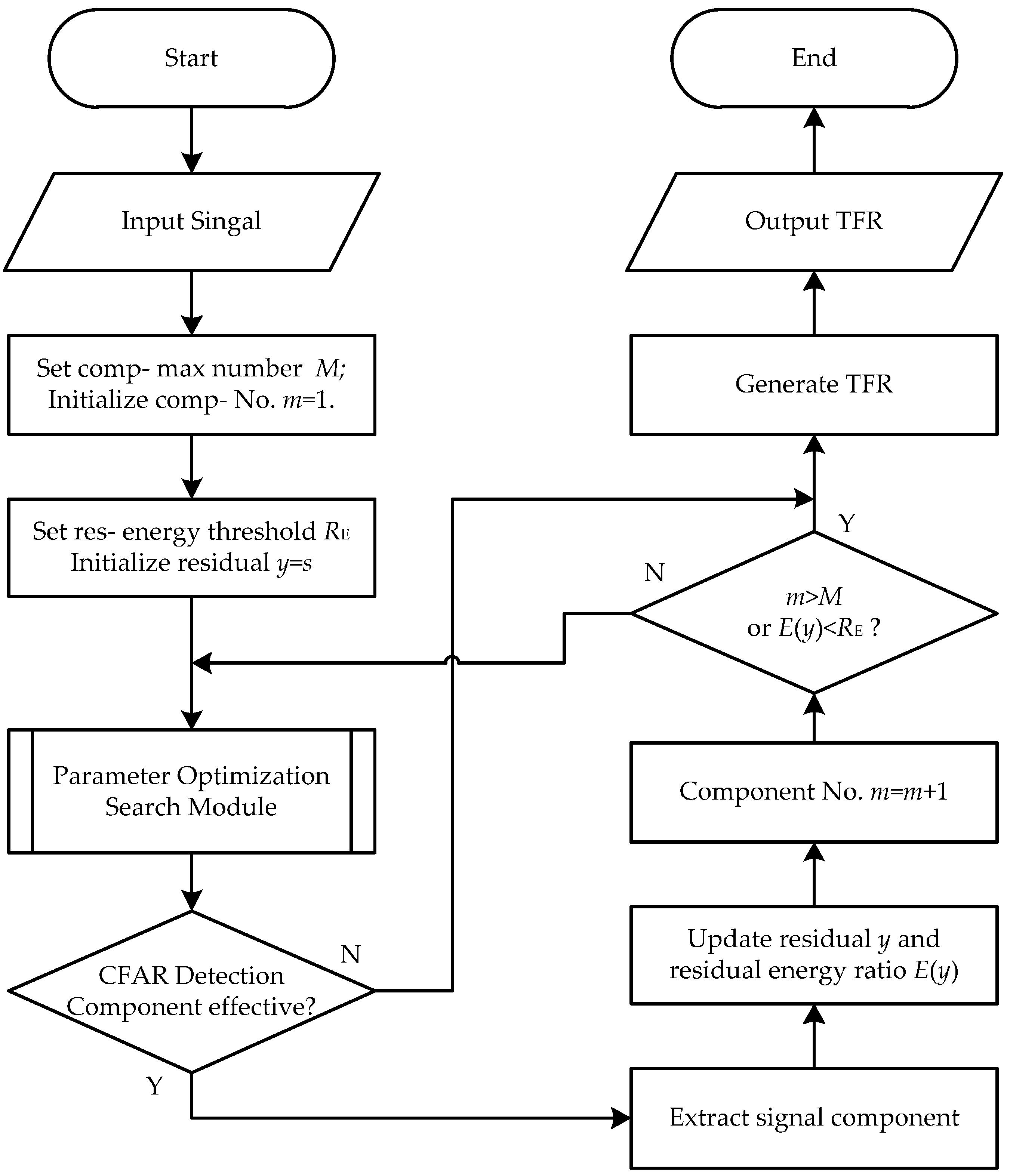
3. FDE-AJTF Procedure

The procedure of the FDE-AJTF method is presented in Figure 1.

The residual energy threshold $R_E$ is the minimum of residual energy ratio, and when the residual energy ratio $E\left(y\right)$ is less than $R_E$, the loop is broken, as shown in Figure 1. To ensure the components are extracted completely, a small threshold $R_E$ is needed, such as 0.1%, i.e., −30 dB, or less than that. However, on the other hand, a small threshold may lead to error component extraction. In fact, when dealing with an unknown signal, the exact residual energy threshold cannot be determined, and that is why the CFAR detection is essential.

During this procedure, the fitness comparison, parameter updating, and choices are completed in the parameter optimization search module. To increase the search speed and global optimal capability, the genetic algorithm (GA) [27], particle swarm optimization (PSO) algorithm [34], ant colony optimization (ACO) [35], etc., can be adopted.

Three break conditions are used to ensure the effectiveness and the convergence of component extraction, in the loop of component extraction, and residual updating. The first break condition is the component number, the second is the residual energy ratio, and the third is the CFAR detection. CFAR detection is used to judge the effectiveness of the extracted components, if one extracted component fails in the CFAR, then such a component will be judged to be ineffective and abandoned, and the loop is broken. The detection threshold becomes lower and more components might pass detection with the constant alarm probability increasing.

The time frequency representation (TFR) is generated as follows: Subsequent to estimating the parameters of each component, the intensities and phase parameters are easily obtained as discussed in Section 2.2.2, and the relationship of time and frequency is as follows:

$$f(t)={\displaystyle {\sum }_{n=1}^{N_{\mathrm{p}}}n{\widehat{a}}_n{t}^{n-1}}$$

(17)

where $f(t)$ is the frequency of the extracted signal.

Then, the distribution of each component on the TFR plane is a $\sin c(·)$ function with the component intensity in the frequency dimension, whose time center is in accordance with its time-frequency curve in the time dimension.

4. Simulation and Experimental Test

4.1. Simulation and Analysis

The simulation data were composed of four three-order PPS components with sample length $N=512$. To compare the decomposition effects, three comparisons were simulated and analyzed between the two fitness and component extraction modes in the classical and FDE AJTF methods, between the basis functions with and without the time window, and between the component extractions with and without CFAR detection. During these simulations, the three-order phase function and PSO algorithm were adopted in both the classical and FDE methods. Furthermore, the product form of CPF (PCPF) method was adopted in the comparisons as a reference.

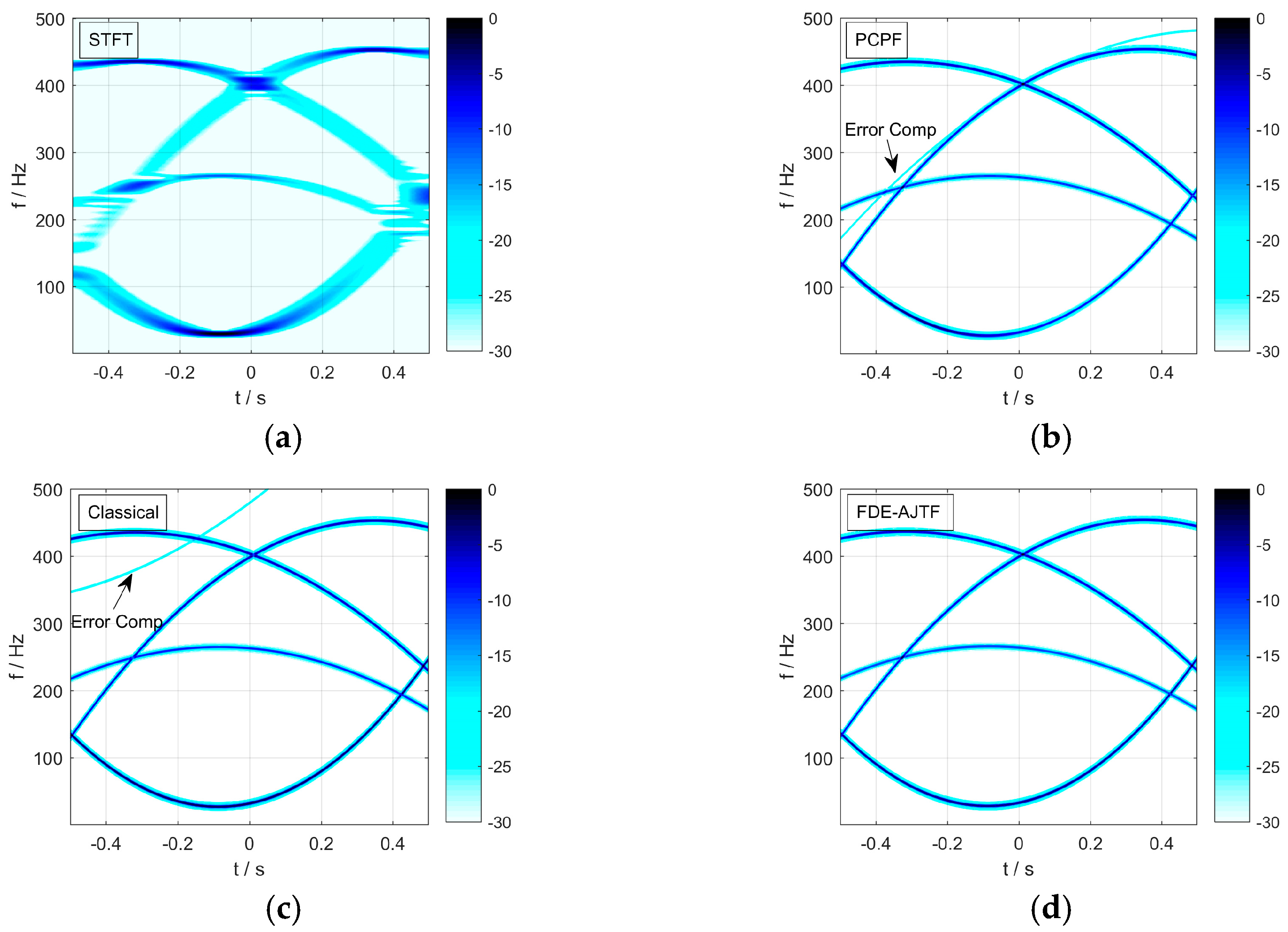
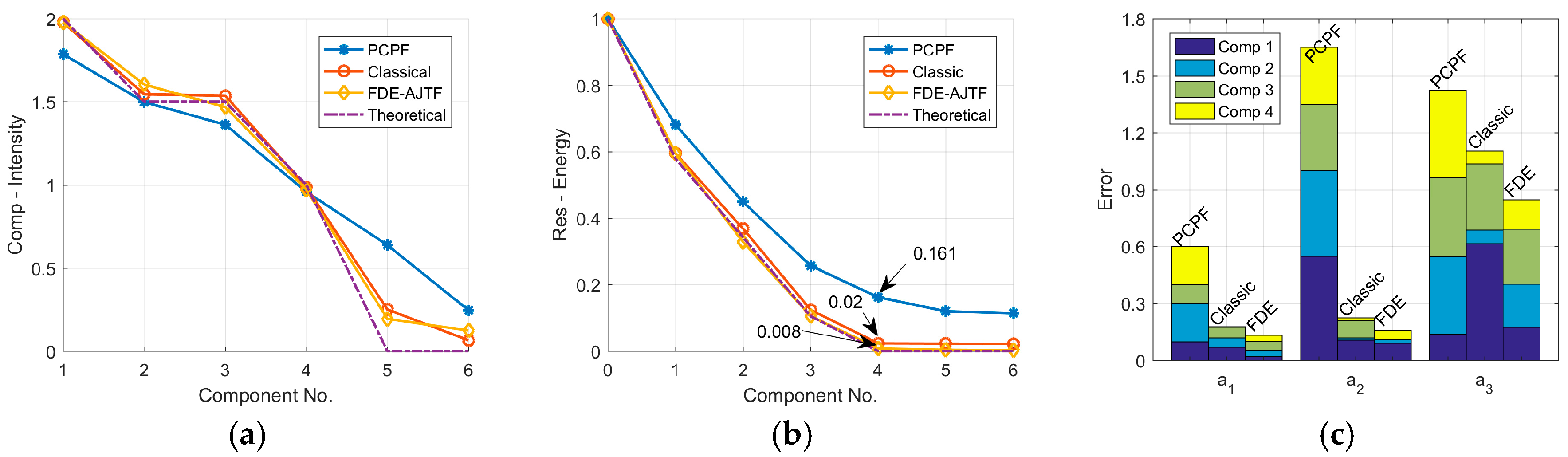
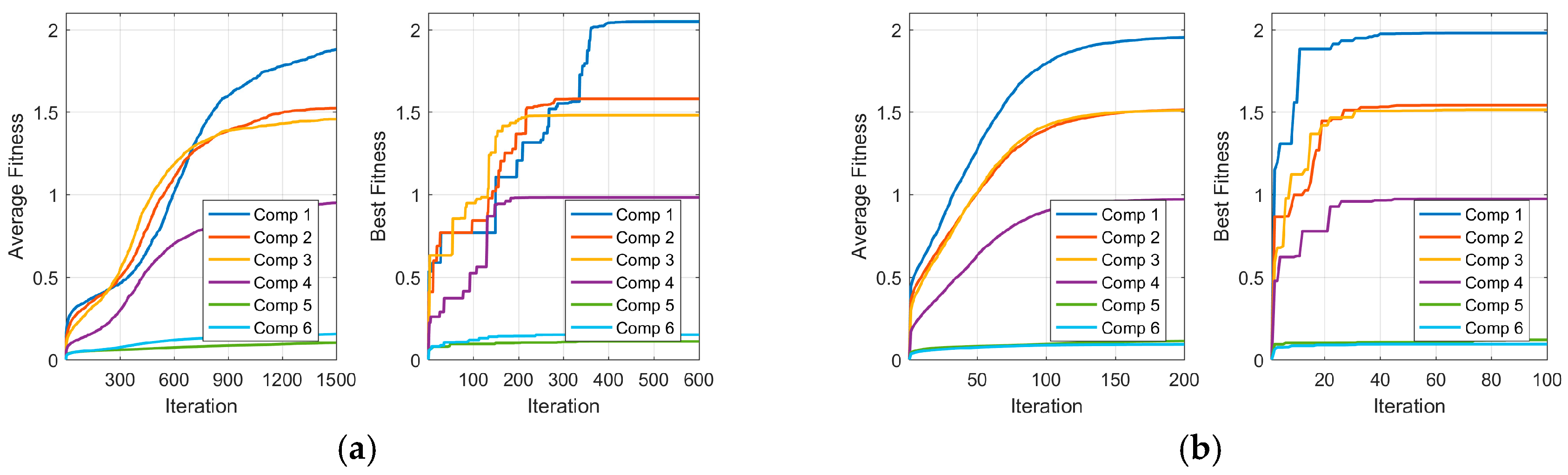
4.1.1. Comparison between Two Fitness and Component Extraction Modes in Classical and FDE AJTF Methods

The parameters of four three-order PPS components are shown in

Table 1. Parameters of four components.

	Intensity	a1	a2	a3	Energy Ratio
Component 1	2.0	32.1	55.6	212.4	42.11%
Component 2	1.5	398.2	156.6	−149.3	23.68%
Component 3	1.5	403.9	−98.2	−102.2	23.68%
Component 4	1.0	262.8	−23.1	−91.5	10.53%

, and the simulating time was from −0.5 s to 0.5 s.

The simulated signal was the linear sum of the four components with parameters in Table 1. Four methods were used to process this signal: STFT, PCPF, classical AJTF, and FDE-AJTF; six components were extracted in the latter three methods. The PSO algorithm had 500 particles both in the classical and FDE AJTF methods, while the iterations of them were different than the 1500 iterations in the classical AJTF and only 200 in the FDE-AJTF. The time frequency decomposition results, in essence TFRs, are shown in Figure 2, and the displayed dynamic range of energy is 30-dB.

Figure 2a demonstrates the general trend of each component displayed by STFT, while the resolution was low due to the time window in STFT. Conversely, in Figure 2b–d, the four components were extracted with higher resolutions than STFT. However, in the case of a 30-dB dynamic range, one error component, i.e., the fifth one, was extracted by both PCPF and classical AJTF, as shown in Figure 2b,c respectively. Figure 2d shows the decomposition result of FDE-AJTF had the best accuracy without any error component. In fact, six components were extracted both in Figure 2c,d respectively, because the loop was set to continue six times. Whereas, no error component is shown in Figure 2d when the dynamic displaying range was 30 dB, due to the smaller intensities of the other two error components than those in the classical method.

The accuracies of three decomposition methods, the intensities of components, the residual energy ratios and the parameter estimation errors for analysis and comparison are shown in Figure 3.

Comparing the theoretical value in Figure 3a, the component intensities estimated by classical and FDE AJTF were more accurate than that by PCPF. Figure 3b, after four components are extracted, show that the energy ratio of the residual signal in FDE-AJTF was 0.8%, while that in the classical AJTF and PCPF were 2% and 16.1%, respectively. The estimation errors of three phase parameters are shown in Figure 3c, and it is evident that the FDE-AJTF led to the least errors of the three. These estimation errors were the reason for the phenomenon in the former two figures.

According to the results in Figure 2 and Figure 3, although 1500 iterations were taken in classical AJTF, the FDE-AJTF, within 200 iterations, performed better. The average and best fitness variations are shown in Figure 4.

Figure 4 shows the best fitness achieved the maximum within 40 iterations and the average fitness got high values steadily within less than 200 iterations in the FDE-AJTF, whereas in the classical AJTF, to reach the maximum of the best fitness, more than 400 iterations were necessary, and to obtain a stable, high average fitness more than 1500 iterations were needed.

The computation burdens of the classical and FDE AJTF methods in this simulation were calculated and shown in

Table 2. Computation burden of classical AJTF and FDE-AJTF.

		Classical AJTF		FDE-AJTF
Signal Length		$N_a$	512	$N_a$	512
Dimension		$N_{\dim }$	3	${N^{\prime }}_{\dim }$	2
Particle		$N_{\mathrm{par}}$	500	$N_{\mathrm{par}}$	500
Iteration		$N_{\mathrm{iter}}$	1500	${N^{\prime }}_{\mathrm{iter}}$	200
Fitness calculate once	Add	$N_a$	500	$N_{a}lo{g}_2{N}_a$	4608
	Multiply	$N_a$	500	$\frac{N_a}{2}lo{g}_2{N}_a$	2304
Velocity update once	Add	$4N_{\dim }{N}_{\mathrm{par}}$	6000	$4{N^{\prime }}_{\dim }{N}_{\mathrm{par}}$	4000
	Multiply	$5N_{\dim }{N}_{\mathrm{par}}$	7500	$5{N^{\prime }}_{\dim }{N}_{\mathrm{par}}$	5000
Position update once	Add	$N_{\dim }{N}_{\mathrm{par}}$	1500	${N^{\prime }}_{\dim }{N}_{\mathrm{par}}$	1000
	Multiply	$N_{\dim }{N}_{\mathrm{par}}$	1500	${N^{\prime }}_{\dim }{N}_{\mathrm{par}}$	1000
Total computation	Add	$N_{\mathrm{iter}}\left(5N_{\dim }{N}_{\mathrm{par}}+N_a\right)$	$1.20\times {10}^7$	${N^{\prime }}_{\mathrm{iter}}\left(\begin{array}{c}5{N^{\prime }}_{\dim }{N}_{\mathrm{par}}\\ + N_{a}lo{g}_2{N}_a\end{array}\right)$	$1.92\times {10}^6$
	Multiply	$N_{\mathrm{iter}}\left(6N_{\dim }{N}_{\mathrm{par}}+N_a\right)$	$1.43\times {10}^7$	${N^{\prime }}_{\mathrm{iter}}\left(\begin{array}{c}6{N^{\prime }}_{\dim }{N}_{\mathrm{par}}\\ + N_a/2\ast lo{g}_2{N}_a\end{array}\right)$	$1.66\times {10}^6$
Ratio	Add		6.25		1
	Multiply		8.60		1

.

The computation differences of the two methods were in the parameter search process that included fitness calculation, velocity, and position update. The details of the PSO algorithm are shown in [28]. According to Table 2, the multiplication computation of classical AJTF was more than seven times larger than that of the FDE-AJTF in this simulation. Therefore, in the FDE-AJTF method, due to one search dimension being ignored, the parameter search speed became much faster with the estimation accuracy improved. The PCPF had the least computation burden, but its accuracy was the worst.

4.1.2. Comparison between the Basis Functions with and without Time Windows

To simulate the appearance and vanishing of different components, four time windows were used. The start and end of the time windows are shown in

Table 3. Time windows of components.

	Start (s)	End (s)
Component 1	−0.3	0.3
Component 2	−0.5	0.5
Component 3	−0.5	0.2
Component 4	−0.4	0.4

. The whole simulating time was from −0.5 s to 0.5 s, and other parameters were the same as in Table 1.

The TFRs obtained by four methods are shown in Figure 5. Synonymous with the former simulation, six components were extracted in the latter three methods, and the dynamic range of Figure 5 is 30-dB.

The general trend of each component with low resolution was displayed by STFT, in Figure 5a. Three effective components were extracted with an error component, in Figure 5b, while a useful component with the least intensity was lost. Four useful components and an error component were extracted, as shown in Figure 5c. However, both in Figure 5b,c, the start and end of these components were not considered, whereas in Figure 5d it is obvious that the decomposition result obtained by the FDE-AJTF was in accord with the TFR in Figure 5a and the parameters in Table 3 due to the time window on the basis function, which was more effective and accurate than these other methods. The error component in Figure 5d was located at the position of the first component, although its time window had errors, and it could be removed by CFAR detection, which is discussed in the next simulation.

The residual energy downward trends of the three methods are shown in Figure 6.

Displayed in Figure 6, after four components were extracted, the residual energy in FDE-AJTF dropped to 2.9%, which was close to theoretical zero, while the residual energy downward trends of the other two methods had greater deviations. It was evident that the accuracy and effectiveness of the component decomposition were increased by the time window on the basis function.

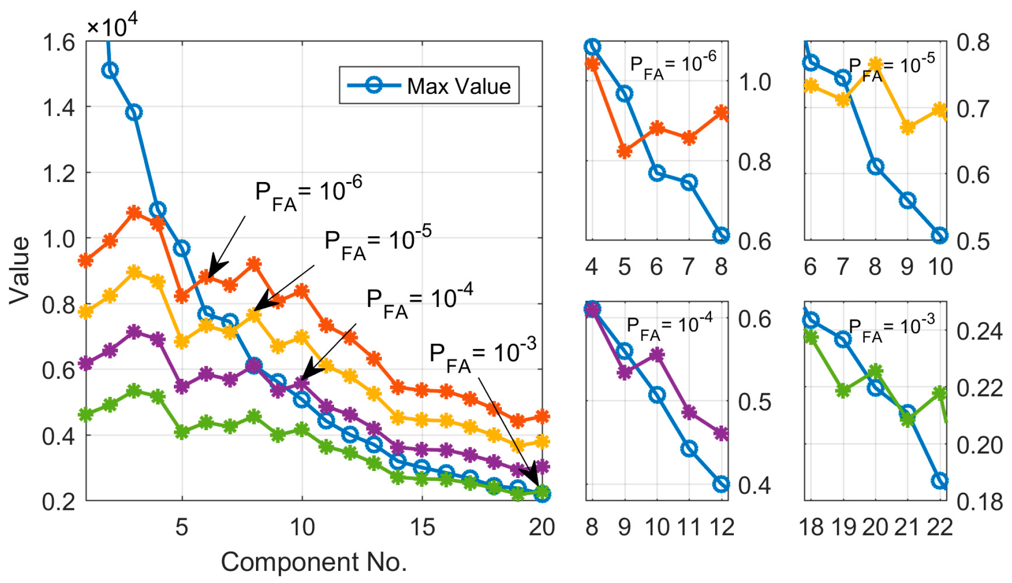
4.1.3. Comparison between Component Extraction with and without CFAR Detection

To illustrate the effect of CFAR detection and to compare the anti-noise performances of different methods, a white noise was mixed with the original signal. Moreover, to one certain component, the other three components could be counted as clutters. The intensities of components and noise were shown in

Table 4. Four PPS components parameters.

	Intensity	SNR (dB)	SCNR (dB)	Energy Ratio
Component 1	2.0	−3.75	−5.74	21.05%
Component 2	1.5	−6.25	−8.72	11.84%
Component 3	1.5	−6.25	−8.72	11.84%
Component 4	1.0	−9.78	−12.56	5.26%
Noise	$\sqrt{9.5}$			50.00%

, in which the SNRs and signal clutter noise ratios (SCNRs) of each component were shown as well. The other parameters were the same as the former simulation.

The CA-CAFR was adopted in the component extraction of FDE-AJTF with constant false alarm probability $P_{\mathrm{FA}}={10}^{-4}$, and detection unit length $N_{\mathrm{CFAR}}=N/4=128$. The TFRs obtained by four methods are shown in Figure 7. During this simulation, six components were extracted as well, and a dynamic range for Figure 7 was 30 dB.

Four components were influenced seriously by the noise, as shown in Figure 7a, while the dynamic range was 40 dB, because the four components cannot be recognized at 30 dB. Six components were extracted by PCPF in Figure 7b, but only the first one was effective. While in Figure 7c, three effective components with two errors were extracted by classical AJTF, the last useful component with the least intensity was lost. Four effective components were extracted accurately, as shown in Figure 7d, by the FDE-AJTF, and their time windows were estimated as well. The fifth component was an error, and it was detected by CFAR, as shown in Figure 8b.

The residual energy downward trends and the CFAR detection result are shown in Figure 8.

Extrapolating from Figure 8a, it is evident that, after four components were extracted, the residual energy of FDE-AJTF was 53.2%, which is close to the theoretical value of 50%. When extracting the first two components, the residual energies were below the theoretical value, which was caused by the estimation errors of intensities and time windows. To illustrate the effect of CFAR detection, only the component effectiveness was judged, and the loop was not broken. Figure 8b shows the fifth component, in essence. The error in Figure 7d, and the sixth component were both detected as ineffective. Thus, in the normal FDE-AJTF procedure in Figure 1, when the fifth component did not pass the CFAR detection, this component was abandoned, and the loop was stopped. Therefore, by the CFAR detection in component extraction, the effectiveness of each component was ensured, and the noise influence was reduced, furthermore, the convergence speed was increased.

4.2. Experimental Test

The measured data were a pulse of a high resolution ISAR echo of a moving ship, but, unfortunately, the ship target was uncooperative and its motions and scattering points were unknown. The components with different parameters were caused by the different reflectors on the ship. Here, although the parameters of this echo piece were unknown, it can be used to extract the components, and to compare the performances of the classical and FDE AJTF methods. The data length was $N=1500$.

During this experimental test, the PSO algorithm within 1500 particles was adopted both in the classical and FDE AJTF method, with 3000 iterations in the classical AJTF method and 600 iterations in the latter. Moreover, four constant alarm probabilities, in essence $P_{\mathrm{FA}}={10}^{-3},{10}^{-4},{10}^{-5}, \mathrm{and} {10}^{-6}$, were adopted in the CFAR detection of FDE-AJTF. The TFRs obtained by STFT, classical, and FDE AJTF are shown in Figure 9 within a 25 dB dynamic range.

Displayed in Figure 9a, several components are included with the rough trends obtained by STFT, where the labeled strong component was used to compare the effects between the two methods. Twenty components were extracted by classical AJTF and contained in the TFR, as shown in Figure 9b, in which several weak and ineffective components were extracted repeatedly while the labeled component was too weak to recognize. Conversely, in Figure 9c, in the case of $P_{\mathrm{FA}}={10}^{-4}$, only nine components were extracted, and the loop was brought to a stop by CFAR detection. Compared with the Figure 9a, the main components and overall trend were represented by these nine components, and the labeled component was obvious.

The downward trends of residual energy and component intensity are shown in Figure 10, while the CFAR detection results with these four ratios were shown in Figure 11.

In Figure 10, the residual energy downward trend of the FDE-AJTF method was much faster than the classical one. The residual energy dropped to 13.9% after nine components were extracted by the FDE-AJTF method, while they dropped to 47% by the classical method, and even 20.4% after 25 components were extracted. Meanwhile, compared with the FDE-AJTF within 600 iterations, the component intensity trend was not stable in the classical AJTF method, although 3000 iterations were adopted in it. It is illustrated that many errors existed in the parameter estimation of the classical method, and the robustness of the FDE-AJTF method was much better than the classical one.

The value maximums in the component extraction and detection thresholds within different $P_{\mathrm{FA}}$ are shown in Figure 11. With the false alarm probability increasing, the threshold became lower and more components were effectively detected, when $P_{\mathrm{FA}}={10}^{-4}$, the components from the tenth one were ineffectively detected, as shown in Figure 9c. Above all, the decomposition result of the FDE-AJTF method was much more accurate and effective than the classical method.

As shown in Table 2, to extract one component in this experimental test, the computation burden of FDE-AJTF method was less than 20% of the classical method, furthermore, the components number of FDE-AJTF method was less than 50%. Therefore, the whole computation of the FDE-AJTF method was less than 10% of the classical method with more accuracy, effectiveness, and robustness.

5. Conclusions

The high-resolution radar echo of a maneuvering target is a multicomponent polynomial phase signal (mc-PPS), which should be processed by time frequency analysis methods of which the adaptive joint time frequency (AJTF) method is the most effective. However, with the improvement of radar resolution and increases to the synthetic period, classical time frequency analysis methods including AJTF cannot satisfy the increasing requirements. To address these problems, a novel frequency domain extraction-based AJTF (FDE-AJTF) decomposition method was proposed, which had three improvements. First, the maximum frequency spectrum of the phase compensation signal was taken as the fitness function, while the fitness comparison, component extraction, and residual updating were operated in the frequency domain. Through these means, the searching rate obviously increased with one dimension ignored in the parameter estimation, while the accuracy and robustness of component extraction increased with the impacts of estimation error and noise reduction. Second, to solve the problem of uncertain signal component time, the time window was adopted as the basis function, and the accuracies of the parameter estimation and component extraction were enhanced. Finally, the effectiveness of the extracted components was improved by CFAR detection applied in component extraction, and the impact of noise was reduced, while the convergence speed was increased. The performance superiorities of the FDE-AJTF method were verified through a comparison with the classical method in a series of simulations and experimental tests.

References

1. Chen, V.C.; Li, F.; Ho, S.S.; Wechsler, H. Micro-Doppler effect in radar: Phenomenon, model, and simulation study. IEEE Trans. Aerosp. Electr. Syst. 2006, 42, 2–21. [Google Scholar] [CrossRef]
2. Liu, Y.; Zhang, S.; Zhu, D.; Li, X. A novel speed compensation method for ISAR imaging with low SNR. Sensors 2015, 15, 18402–18415. [Google Scholar] [CrossRef] [PubMed]
3. Wang, Y.; Jiang, Y. ISAR imaging of a ship target using product high-order matched-phase transform. IEEE Geosci. Remote Sens. Lett. 2009, 6, 658–661. [Google Scholar] [CrossRef]
4. Lao, G.; Liu, G.; Wu, X. The modeling and simulation of spaceborne SAR moving vessel imaging based on Matlab class. In Proceedings of the International Conference on Frontiers of Manufacturing Science and Measuring Technology (FMSMT), Taiyuan, China, 24–25 June 2017; Atlantis Press: Paris, France, 2017; Volume 130, pp. 1583–1586, ISBN 978-94-6252-331-9. [Google Scholar]
5. Barbarossa, S.; Scaglione, A.; Giannakis, G.B. Product high-order ambiguity function for multicomponent polynomial-phase signal modeling. IEEE Trans. Signal Process. 1998, 46, 691–708. [Google Scholar] [CrossRef]
6. Pham, D.S.; Zoubir, A.M. Analysis of multicomponent polynomial phase signals. IEEE Trans. Signal Process. 2007, 55, 56–65. [Google Scholar] [CrossRef]
7. Zhang, X. Modern Signal Processing, 3rd ed.; Tsinghua University Press: Beijing, China, 2015; pp. 294–310. ISBN 978-7-302-40869-7. [Google Scholar]
8. Boashash, B.; Ristic, B. Polynomial time-frequency distribution and time-varying higher order spectra: Application to the analysis of multicomponent FM signals and to the treatment of multiplicative noise. Signal Process. 1998, 67, 1–23. [Google Scholar] [CrossRef]
9. Sun, K.; Jin, T.; Yang, D. An Improved Time-Frequency Analysis Method in Interference Detection for GNSS Receivers. Sensors 2015, 15, 9404–9426. [Google Scholar] [CrossRef] [PubMed]
10. Friedlander, B.; Francos, J.M. Estimation of amplitude and phase parameters of multicomponent signals. IEEE Trans. Signal Process. 1995, 43, 917–926. [Google Scholar] [CrossRef]
11. Djurovic, I.; Stankovic, L. Quasi maximum likelihood estimator of polynomial phase signals. IET Signal Process. 2014, 13, 347–359. [Google Scholar] [CrossRef]
12. Djurovic, I.; Simeunovic, M. Review of the quasi-maximum likelihood estimator for polynomial phase signals. Digit. Signal Process. 2018, 72, 59–74. [Google Scholar] [CrossRef]
13. Peleg, S.; Porat, B. Estimation and classification of polynomial-phase signals. IEEE Trans. Inf. Theory 1991, 37, 422–430. [Google Scholar] [CrossRef]
14. Wang, Y.; Abdelkader, A.C.; Zhao, B.; Wang, J. ISAR imaging of maneuvering targets based on the modified discrete polynomial-phase transform. Sensors 2015, 15, 22401–22418. [Google Scholar] [CrossRef] [PubMed]
15. Jing, F.; Si, W.; Jiao, S. A hybrid LVD-HAF method of quadratic frequency-modulated signals. In Proceedings of the Applied Computational Electromagnetics Society Symposium, Italy (ACES), Florence, Italy, 26–30 March 2017; ISBN 978-1-5090-5335-3. [Google Scholar]
16. Zheng, J.; Su, T.; Zhu, W.; Zhang, L.; Liu, Z.; Liu, Q. ISAR imaging of nonuniformly rotating target based on a fast parameter estimation algorithm of cubic phase signal. IEEE Trans. Geosci. Remote Sens. 2015, 53, 4727–4740. [Google Scholar] [CrossRef]
17. Djurovic, I.; Simeunovic, M.; Wang, P. Cubic Phase Function: A Simple Solution to Polynomial Phase Signal Analysis. Elsevier Signal Process. 2017, 135, 48–66. [Google Scholar] [CrossRef]
18. Popovica, V.; Djurovica, I.; Stankovica, L.; Thayaparanb, T.; Dakovica, M. Autofocusing of SAR images based on parameters estimated from the PHAF. Signal Process. 2010, 90, 1382–1391. [Google Scholar] [CrossRef]
19. Djurovic, I.; Simeunovic, M.; Djukanovic, S.; Wang, P. A hybrid CPF-HAF estimation of polynomial-phase signals: Detailed statistical analysis. IEEE Trans. Signal Process. 2012, 60, 5010–5023. [Google Scholar] [CrossRef]
20. Djurovic, I.; Ioana, C.; Thayaparan, T.; Stankovic, L.; Wang, P.; Popovic, V.; Simeunovic, M. Cubic-phase function evaluation for multicomponent signals with application to SAR imaging. IET Signal Process. 2010, 4, 371–381. [Google Scholar] [CrossRef]
21. Kulkarni, R.; Rastogi, P. Multiple phase estimation in digital holographic interferometry using product cubic phase function. Opt. Lasers Eng. 2013, 51, 1168–1172. [Google Scholar] [CrossRef]
22. Trintinalia, L.; Ling, H. Joint time-frequency ISAR using adaptive processing. IEEE Trans. Antennas Propag. 1997, 45, 221–227. [Google Scholar] [CrossRef]
23. Qian, S.; Chen, D. Signal representation using adaptive normalized Gaussian functions. Signal Process. 1994, 36, 1–11. [Google Scholar] [CrossRef]
24. Mallat, S.G.; Zhang, Z. Matching pursuits with time-frequency dictionaries. IEEE Trans. Signal Process. 1993, 41, 3397–3415. [Google Scholar] [CrossRef]
25. Thayaparan, T.; Brinkman, W.; Lampropoulos, G. Inverse synthetic aperture radar image focusing using fast adaptive joint time–frequency and three-dimensional motion detection on experimental radar data. IET Signal Process. 2010, 4, 382–394. [Google Scholar] [CrossRef]
26. Yang, G.; He, Z. Improvement for ISAR Imaging Algorithms of Ship Targets. Mod. Def. Technol. 2013, 1, 47–52. [Google Scholar] [CrossRef]
27. Brinkman, W.; Thayaparan, T. Focusing inverse synthetic aperture radar images with higher-order motion error using the adaptive joint-time-frequency algorithm optimised with the genetic algorithm and the particle swarm optimisation algorithm-comparison and results. IET Signal Process. 2010, 4, 329–342. [Google Scholar] [CrossRef]
28. Li, Y.; Fu, Y.; Li, X.; Lewei, L. ISAR imaging of multiple targets using particle swarm optimization—Adaptive joint time frequency approach. IET Signal Process. 2010, 4, 343–351. [Google Scholar] [CrossRef]
29. Qian, S. Introduction to Time-Frequency and Wavelet Transforms; China Machine Press: Beijing, China, 2005; pp. 142–143. ISBN 7-111-15834-2. [Google Scholar]
30. Wu, D. Analysis of Signals and Linear Systems, 4th ed.; Higher Education Press: Beijing, China, 2005; pp. 150–152. ISBN 978-7-04-017401-4. [Google Scholar]
31. Bao, Z.; Xing, M.; Wang, T. Radar Imaging Technology; Publishing House of Electronics Industry: Beijing, China, 2005; pp. 95–97, 142–143. ISBN 7-121-01072-0. [Google Scholar]
32. Hu, G. Digital Signal Processing, 3rd ed.; Tsinghua University Press: Beijing, China, 2015; pp. 269–273. ISBN 978-7-302-29757-4. [Google Scholar]
33. Richards, M.A. Fundamentals of Radar Signal Processing, Simplified Chinese Translation Edition; Publishing House of Electronics Industry: Beijing, China, 2008; pp. 260–268. ISBN 978-7-121-06896-6. [Google Scholar]
34. Hassan, R.; Cohanim, B.; Weck, O.D.; Venter, G. A comparison of particle swarm optimization and the genetic algorithm. In Proceedings of the AIAA/ASME/ASCE/AHS/ASC Structures, Structural Dynamics & Materials Conference, Austin, TX, USA, 18–21 April 2005. [Google Scholar] [CrossRef]
35. Dorigo, M.; Stutzle, T. Ant Colony Optimization; Simplified Chinese Translation Edition; Tsinghua University Press: Beijing, China, 2007; pp. 65–68. ISBN 978-7-302-13887-7. [Google Scholar]
Figure 1. FDE-AJTF procedure.
Remotesensing 10 00266 g001
Figure 2. TFRs obtained by four methods. (a) STFT; (b) PCPF; (c) classical AJTF; and (d) FDE-AJTF method.
Remotesensing 10 00266 g002
Figure 3. Accuracy comparison. (a) Components intensities; (b) residual energy ratios; and (c) parameter estimation errors.
Remotesensing 10 00266 g003
Figure 4. Average and best fitness variations. (a) Classical AJTF method; and (b) the FDE-AJTF method.
Remotesensing 10 00266 g004
Figure 5. TFRs obtained by four methods. (a) STFT; (b) PCPF; (c) Classical AJTF; and (d) FDE-AJTF with time windows.
Remotesensing 10 00266 g005
Figure 6. Residual energy downward trends.
Remotesensing 10 00266 g006
Figure 7. TFRs obtained by four methods. (a) STFT; (b) PCPF; (c) Classical AJTF; and (d) FDE-AJTF with time window.
Remotesensing 10 00266 g007
Figure 8. Residual energy downward trends and CFAR detection result. (a) Residual energy downward trends; and (b) the CFAR detection result.
Remotesensing 10 00266 g008
Figure 9. Time frequency decomposition results. (a) STFT; (b) classical AJTF method; and (c) FDE-AJTF method.
Remotesensing 10 00266 g009
Figure 10. Downward trends of residual energy and component intensity.
Remotesensing 10 00266 g010
Figure 11. FDE-AJTF CFAR detection result.
Remotesensing 10 00266 g011