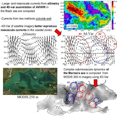
Reconstructing Large- and Mesoscale Dynamics in the Black Sea Region from Satellite Imagery and Altimetry Data—A Comparison of Two Methods

Abstract

Two remote sensing methods, satellite altimetry and 4D-Var assimilation of satellite imagery, are used to compute surface velocity fields in the Black Sea region. Surface currents derived from the two methods are compared for several cases with intense mesoscale and large-scale dynamics during low wind conditions. Comparison shows that the obtained results coincide well quantitatively and qualitatively. However, satellite imagery provides more reasonable results on the spatial variability of coastal dynamics than altimetry data. In particular, this is related to the reconstruction of eddy coastal dynamics, such as Black Sea near-shore anticyclones. Current streamlines in these eddies are not closed near the coast in altimetry data, which we relate to the extrapolation during mapping procedure in the absence of coastal along-track measurements. On the other hand, in offshore areas, imagery-derived currents can be underestimated due to the absence of thermal contrasts and smoothing during the procedure of the 4D-Var assimilation. Wind drift currents are another source of inconsistency, as their impact is directly observed in satellite imagery but absent in altimetry data. The advantage of the 4D-Var method for reconstructing coastal dynamics is used to compute surface currents in the Marmara Sea on the base of 250 m resolution Modis optical data. The results reveal the very complex dynamics of the basin, with a large number of mesoscale and sub-mesoscale eddies. 4D-Var assimilation of Modis imagery is used to obtain information about dynamic characteristics of these small eddies with radiuses of 4–10 km.

1. Introduction

Current velocity is an essential parameter for studying large-scale and mesoscale ocean dynamics, estimating heat and salt transport, and other important oceanographic tasks. It is needed for a lot of oceanographic applications: maritime safety, oil spill propagation, dynamics modeling, and many others. Direct measurements of current velocity by in situ methods are rather sparse and thus have low spatial–temporal resolution. Remote sensing is a good alternative, which allows us to regularly determine the surface current over the ice-free world ocean basin.

Today, microwave satellite altimetry is one of the major sources of information about ocean dynamics. Highly accurate satellite altimetry measurements became available after ERS-1 and Topex/Poseidon launched in 1991 and 1992. Altimetry provides regular data about sea level distribution and associated geostrophic currents. Altimetry measurements by satellites have allowed, for the first time in the history of oceanography, to determine the geostrophic circulation of the world ocean, almost in real time [1,2]. These data are widely used in different oceanographic studies, which provide a lot of new insights about large and mesoscale ocean dynamics all over the world [3,4,5]. In the Black Sea region, altimetry data were validated using tide gauges, drifters, hydrology, and satellite imagery data in a series of studies [6,7,8,9,10,11,12,13,14], which show its good capability for reconstructing sea level and current velocity. Altimetry data were used to investigate mechanisms driving the Black Sea’s large [7,15], and mesoscale dynamics [16,17,18,19], their seasonal and interannual variability [12,18,20], and their impact on the basin ecosystem [18,21,22,23]. However, microwave altimetry measurements have several weaknesses. First, one satellite allows us to determine only one component of current velocity (cross-track). Data from several satellites can be used to reconstruct current fields [24,25]; however, the resolution of the mapped data is relatively low due to spatial inter/extrapolation (~12–25 km). Second, altimetry measurements are not available near the coast, and their accuracy in the vicinity of the coast falls down due to inaccurate atmospheric and geophysical corrections [26]. This includes the decrease of quality of the wet tropospheric correction, mapping procedure, mean dynamic topography, and difficulties in the description of barotropic sea level variability [2,27,28,29,30]. Third, altimetry-derived velocities are geostrophic and represent only a part, also very important, of the current velocity [31]. Wind-driven currents are another important part of the surface currents, and should be additionally described using different assumptions [32,33,34,35] to reconstruct total surface currents on the basis of satellite altimetry. Such an approach was used, for example, to simulate drift trajectories or oil spill propagation [34,36], and it was shown that it may perform better than the data assimilative models in [36].

Another source of data, applicable for sea surface current velocity estimation is satellite IR and optical imagery. Optical and thermal features act like tracers, allowing for the reconstruction of current velocity from consecutive satellite images. Radar backscattering data has also been used for feature tracking algorithms in recent years [37]. Sequences of time-ordered images allow for the estimation of two-dimensional image motion as either instantaneous image velocities or discrete image displacements. Primary approaches to estimating velocity fields from image sequences can be divided into two groups [38]: differential methods, which are mostly based on heat or optical flow equations inversion [39,40,41,42,43,44], and the Maximum Cross Correlation (MCC) technique [45,46,47,48,49,50,51,52,53,54,55]. Modern algorithms are complex, sometimes combining several approaches or in situ measurements, e.g., [52,56]. In the Black Sea region, MCC and optical flow methods were used in [46,48,57,58].

In the present study, the estimation of motion on an image sequence is implemented by the 4D-Var data assimilation method [57]. The method is based on the assumption that image intensity evolution can be described by a transport model. It is considered that the main reason for signal changes from one image to another is horizontal advection and the surface velocity field is assumed to vary much more slowly than the temperature field observed in satellite images. The problem is solved by using a variational principle, e.g., the minimization of the discrepancy between model solutions and observations. This gives the possibility of obtaining both the initial temperature distribution and surface velocity field by processing several consecutive satellite images. The main advantage of the velocity estimation from satellite imagery is its high spatial resolution, and availability near the coast, where currents are of the primary importance for economics. The number of devices measuring in the optical and infrared diapason, along with their resolution and accuracy, significantly increases in the latter period. The main weakness of the data is their irregularity, caused by complete obstruction by clouds and the impossibility of determining currents in the absence of gradients of remote sensing brightness, for example, due to solar heating.

In this study, we use two specified approaches (Section 2) to reconstruct surface velocity fields in the Black Sea basin. Surface currents derived from two independent datasets are compared for several cases with intense mesoscale and largescale dynamics (Section 3). Comparison shows that the currents derived from mapped satellite altimetry and satellite imagery coincide well quantitatively and qualitatively. This coincidence was validated in recent studies through altimetry data indicating that the 4D-Var data assimilation method can be effectively used to reconstruct the spatial variability of current velocity on meso- and large spatial scales in coastal basins. In Section 3.7 we use satellite imagery with 250 m resolution to obtain basin-scale surface currents in the small and enclosed Marmara Sea, where mapped altimetry measurements are unavailable. The Marmara Sea is the first connecting link between the Black Sea and the Atlantic Ocean and its circulation is of importance for the interbasin exchange through the Bosphorus strait [8,14,59,60,61,62,63,64]. Observation-based data on the surface currents obtained using 4D-Var assimilation of satellite imagery give the possibility of reconstructing complex mesoscale and sub-mesoscale dynamics in the Marmara Sea.

2. Materials and Methods

2.1. Satellite Altimetry

Satellite altimeters emit microwave impulse in nadir and measure the time of propagation of a signal from altimeter to surface and back. This information, after a series of atmospheric and sea state corrections, including dry and wet tropospheric corrections, ionospheric correction, and electromagnetic correction [2,65], is used to determine the distance between the satellite and the ocean, and, therefore, to find the height of the sea surface above the reference ellipsoid, Sea Surface Height (SSH). The accuracy of the modern altimetry measurements of SSH depends on the accuracy of the orbit positioning and atmospheric corrections and has recently reached 2–5 cm [66]. However, as the wet tropospheric correction largely depends on the microwave passive measurements, which are unavailable in the vicinity of land/ice, the accuracy of SSH decreases near the coast [27].

Surface geostrophic velocity, through the geostrophic balance equation, is related to the gradients of the dynamic topography of the sea, which is equal to the height of the sea surface over the geoid [1]. Geoid height relative to the reference ellipsoid is a major part of SSH spatial variability and should be subtracted from SSH in order to calculate dynamic topography from altimetry measurements. This task is still a challenge as modern gravimetric missions have insufficient spatial resolution for oceanographic needs [67,68]. To avoid this problem, altimetry measurements are distributed in terms of Sea Level Anomalies (SLA), which are defined as deviations of full dynamic topography from a mean dynamic topography, averaged over 1993–2012 (MDT). Full dynamic topography, h, is, therefore, the sum of Mean Dynamic Topography H (MDT) for the 1993–2012 period and SLA h′: h = H + h′. In this work we use synthetic MDT of the Black Sea computed from altimetry, drifting buoys, and hydrological data [69]. The computation of MDT in the coastal zone is another challenge as it is based on drifter measurements [67,68,69,70], which are mostly situated offshore in the deep part of the ocean.

Combining measurements from two [24] or more [25] satellites allows us to obtain daily gridded maps of SLA (MSLA) from along-track altimetry data. The spatial resolution of this data is 1/4 degree for the World Ocean area. However, for the Black Sea region, special methods were developed in CLS (Collected Localization Satellite) that allow us to obtain a regional high-resolution dataset of SLA with 1/8° degree spatial resolution. The MSLA used here were produced by Ssalto/Duacs and distributed by Aviso, with support from Cnes (http://www.aviso.oceanobs.com/duacs/). The mapping procedure is based on spatio-temporal optimal interpolation, which may provide additional error and smoothing of the SLA fields [71]. These errors can be particularly significant in coastal areas. In the part of coastal areas where along-track data is unavailable, obtained MDLA is related only to the extrapolation procedure, which cannot resolve complex coastal dynamics. Gradients of absolute dynamic topography define geostrophic velocities through the geostrophic balance equation:

$$u_g=-\frac{g}{f}\frac{\partial h}{\partial y},v_g=\frac{g}{f}\frac{\partial h}{\partial x}$$

(1)

where u_g, v_g are zonal and meridional component of geostrophic velocity, x, y are longitude and latitude, f = 10⁻⁴ s⁻¹ is the Coriolis parameter, and g = 9.8 m·s⁻¹ is the gravitational acceleration. Before the computation of geostrophic velocity, the high-frequency barotropic part of the signal and the effects of the inverse barometer should be subtracted from SLA fields. This is done using barotropic models [71], which has strongly improved their quality in recent years [28].

Altimetry-derived geostrophic velocities in the Black Sea were validated earlier in a number of studies using hydrological data, drifter measurements, and satellite imagery [10,12,69]. Validation showed a reasonable quality of altimetry data for estimating the spatial variability and magnitudes of Black Sea surface currents.

2.2. Surface Currents from Variational Assimilation of Satellite Image Sequences

The basic idea of the 4D-Var variational assimilation technique [57], as well as of most differential optical flow estimation methods, is that the signal strongly changes from one image to another due to the horizontal advection. Under this condition, surface current transfer can be described by the optical flow equation:

$$\frac{\partial T}{\partial t}=-u\frac{\partial T}{\partial x}-v\frac{\partial T}{\partial y}$$

(2)

where T is a sea surface temperature (SST), and u and v are velocity field components.

For the connection of simulated and observed images a cost function is introduced to minimize the difference between them. Generally the issue can be described as finding a solution to the optical flow equation, which minimizes the specified cost function. In practice, the problem requires the introduction of additional regularization terms. One of the conventional approaches in this case is minimizing the gradient and divergence of current velocity. The cost function can be expressed by the formula

$$J\left(T,u,v\right)=\frac{1}{2}{\displaystyle \sum }_{k=1}^N\underset{\Omega }{\overset{ }{{\displaystyle \int }}}{\left(T\left(t_k\right)-T_{obs}\left(t_k\right)\right)}^{2}ds+\frac{\alpha }{2}\underset{\Omega }{\overset{ }{{\displaystyle \int }}}{\left|grad\left(V\right)\right|}^{2}ds+\frac{\beta }{2}\underset{\Omega }{\overset{ }{{\displaystyle \int }}}div{\left(V\right)}^{2}ds$$

(3)

where Ω is the observed region, V = (u, v) is the velocity field, T_obs are observed signal intensities, N is the number of observations, α and β are empirical constants, and t_k is the observation time. Increase of α and β leads to a stronger smoothing of resulting velocity fields.

While simulated temperature flow T(t) can be obtained by Equation (2), integrating the initial fields T₀, u₀ and v₀, it is possible to find the gradient of J via backward adjoint system integration in time [57]:

$$\{\begin{array}{c}\frac{\partial \tilde{T}}{\partial t}+\frac{\partial \left(u\tilde{T}\right)}{\partial x}+\frac{\partial \left(v\tilde{T}\right)}{\partial y}+T-T_{obs}=0\\ \frac{\partial \tilde{u}}{\partial t}-\tilde{T}\frac{\partial T}{\partial x}+\alpha {\nabla }^2\left(u\right)+\beta \left(\frac{{\partial }^{2}u}{\partial x^2}+\frac{{\partial }^{2}v}{\partial x\partial y}\right)=0\\ \frac{\partial \tilde{v}}{\partial t}-\tilde{T}\frac{\partial T}{\partial y}+\alpha {\nabla }^2\left(v\right)+\beta \left(\frac{{\partial }^{2}v}{\partial y^2}+\frac{{\partial }^{2}u}{\partial x\partial y}\right)=0\end{array}$$

(4)

where $\tilde{T}, \tilde{u}, \tilde{v}$ are adjoint variables and the starting conditions are: $\tilde{T}\left(t_N\right)=0, \tilde{u}\left(t_N\right)=0, \tilde{v}\left(t_N\right)=0$. Now the gradient of J is equal to $\left(\tilde{T}\left(t_1\right), \tilde{u}\left(t_1\right), \tilde{v}\left(t_1\right)\right).$ After that, the quasi-gradient descent algorithm is applied to obtain the minimum of J, which is used like a start condition for the next iteration.

The computation scheme is iterative and contains the following steps:

• Choose initial T₀, u_0, v₀ values. Initial fields for the first iteration are: $T_0=T_{obs}\left(t_1\right), u_0=0,v_0=0$.
• Integrate Equation (2) and obtain the corresponding J value.
• Solve adjoint system (4) with the starting conditions $\tilde{T}\left(t_N\right)=0, \tilde{u}\left(t_N\right)=0, \tilde{v}\left(t_N\right)=0$ to calculate the gradient of J.
• Obtain new T₀, u₀ and v₀ as a local minimum of J via quasi-Newton descent.
• Go to step 2 if the required accuracy is not achieved; otherwise, u₀ and v₀ are final resulting velocity field components.

Equations (2)–(4) are approximated by finite differences using the Euler scheme in time and by the central differences in space. The velocity components and temperature field are approximated according to Arakawa’s box method on shifted grids [72]. The temperature values are referenced to the center of boxes, whereas the velocity components are set on their boundaries. The adjoint equations are obtained directly from the finite difference system of the governing equations. Standard quasi-Newton minimization subroutine M1QN3 [73] is used to find the next guess of the initial conditions to problems (2)–(4).

The time step for numerical integration is 15 min. Constants α and β are chosen separately for each situation but usually are about α = 10⁷ s grad and β = 10⁸ s grad. In most situations the number of required iterations is about 1000. In practice, satellite IR image sequences often contain distortions that decrease the quality of the calculations. Besides the presence of cloud-covered fragments and small-scale noise, diurnal temperature variability and diurnal warming in SST fields produce radiance changes from one image to another, not related to dynamical processes, that disturb optical flow equation applying limitations. Thus, an accurate data preprocessing procedure is required to obtain relevant results.

The corresponding steps and methods are as follows:

• Remove cloud-covered regions in conjunction with interactive processing by the operator. Clouds in the AVHHR imagery are detected using a method based on [74], which uses a series of threshold tests in individual AVHRR channels.
• Remove small-scale noise using normalized box filter with 3 × 3 kernel.
• Remove large-scale noise using a high-frequency moving average with a large window size (about 50 × 50) This procedure saves SST gradient structures but removes large-scale differences between observations typical of diurnal temperature variability effects or atmospheric correction error.

The minimum number of required assimilated images is 2. A higher number of images allows us to decrease the noise related to the image distortion (e.g., due to the absence of thermal gradients) and makes the computational process more stable.

In the present study, we used NOAA/AVHRR infrared imagery with a spatial resolution of about ~1.1 km. Data were obtained from the archive of the Marine Hydrophisycal Institute (dvs.net.ru). Simultaneous measurements from several satellites in orbit can provide up to six images of the same fragment of sea surface during a day.

The 250 m MODIS Level-1B dataset containing calibrated and geolocated at-aperture radiances of 0.62–0.67 µm is used for the reconstruction of the Marmara Sea dynamics (MYD02QKM—http://dx.doi.org/10.5067/MODIS/MYD02QKM.006) in Section 3.7. Data were obtained from the LAADS DAAC portal (https://ladsweb.modaps.eosdis.nasa.gov/). For visualization purposes, we used data images from the Worldview portal (https://worldview.earthdata.nasa.gov/), NASA.

Wind velocity at 10 m above the sea surface was obtained from Modern Era Retrospective Analysis for Research and Applications (MERRA) reanalysis [75]. Three-hourly maps with a spatial resolution of 1/2° × 2/3° were used. MERRA is the NASA reanalysis for the satellite era, where a major new version of the Goddard Earth Observing System Data Assimilation System Version 5 (GEOS-5) was applied. The data were downloaded from http://goldsmr2.sci.gsfc.nasa.gov/.

3. Results

Six cases were chosen for the comparison of current velocity reconstructed from satellite imagery and altimetry measurements: two with mesoscale eddies; two with complex mesoscale dynamics; and two basin-scale examples. To minimize the impact of wind-drift velocities on the comparison we choose cases that correspond to weak or moderate wind conditions (wind velocity less than 7 m·s⁻¹). Let us consider these cases one by one.

3.1. Scene 1: Anticyclonic Eddy in the Northwestern Part of the Black Sea on 11 May 2005

Six AVHHR images (three shown in Figure 1a–c) were obtained from 13 to 14 May 2005 in the zone of the so-called Sevastopol eddy, which is one of the places of intense mesoscale dynamics in the Black Sea. A warm jet with SST = 15.4°, rotating anticyclonically around the cold area with SST = 13.6°, was observed in the AVHHR images. This jet is related to the advection of coastal waters by mesoscale anticyclone. The anticyclone is asymmetric and elongated in the southwest–northeast direction, which corresponds to the direction of the largescale Rim current in this area of the basin.

Velocity fields calculated from satellite altimetry and 4D-Var assimilation of AVHHR imagery are shown in Figure 1d,e. Both methods are able to reconstruct the observed anticyclone and its asymmetry. Velocity distribution is also asymmetric, with maximums in the northwest and southeast parts of the eddy. A comparison of meridional sections of zonal velocity (vx) and zonal sections of meridional velocity (vy) across the eddy center (gray lines on Figure 1e) is shown in Figure 1f,g. Amplitudes of meridional velocity obtained by the two methods are almost equal; the maximum, −0.3 m·s⁻¹, is situated near the periphery of the eddy (on about 2/3 radius length). Zonal velocities are slightly biased: They vary from −0.25 m·s⁻¹ to 0.1 m·s⁻¹ for image sequences and from −0.17 m·s⁻¹ to 0.17 m·s⁻¹ for altimetry data. This bias is related to the small differences in the orientation of the anticyclone, computed from two methods. The anticyclone in altimetry data (Figure 1a) is elongated in the west–east direction. At the same time, from the satellite images in Figure 1a–c it can be seen that the eddy is stretched more in the northeast–southwest direction. This corresponds with the results obtained used 4D-Var assimilation (Figure 1e). Therefore, in this case it can be suggested that the eddy form is slightly distorted in altimetry data. This can be related to the mapping procedure and spatial and temporal interpolation of along-track data, which lead to additional smoothing of dynamic topography [71]. Another probable reason is the inaccuracy in MDT, which is hard to obtain precisely near the abrupt continental slope.

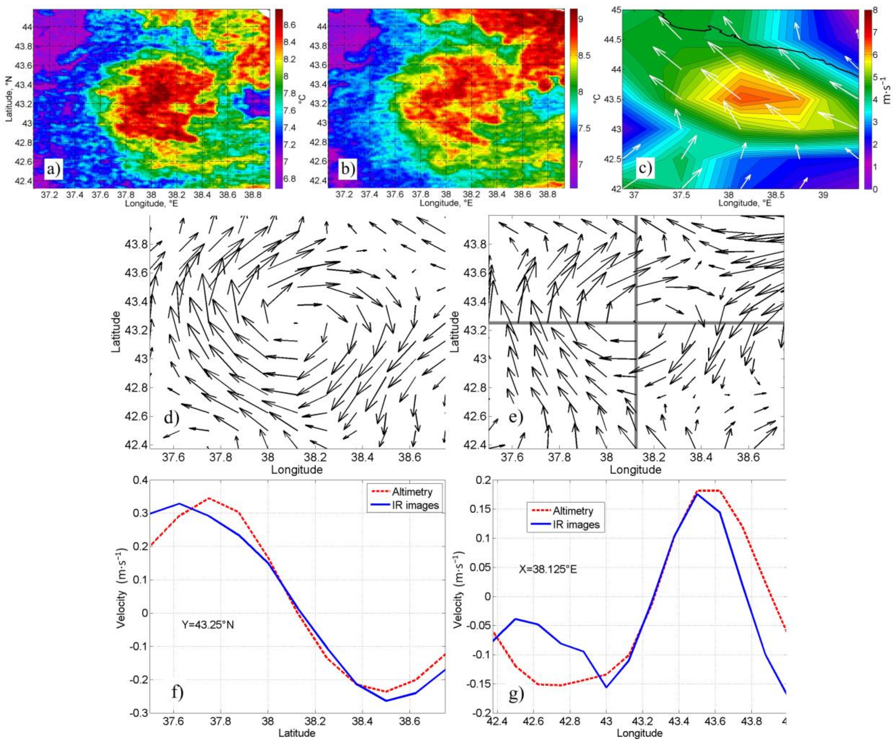
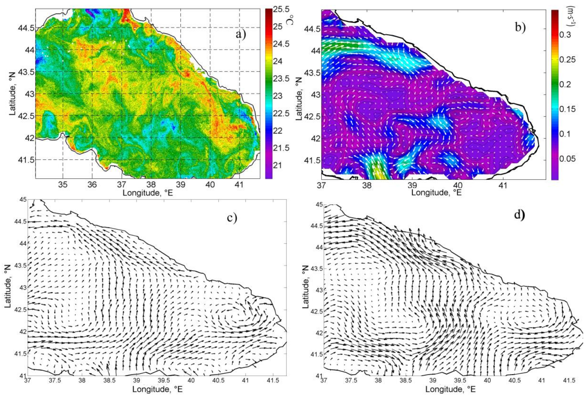
3.2. Scene 2: Anticyclone Eddy in the Eastern Part of the Black Sea

The next scene corresponds to the warm anticyclone, clearly observed in the SST field on 13 and 14 February 2007 (Figure 2a,b). Rarely for the Black Sea, this anticyclone is situated to the right of the Rim current flow and can be called an open ocean eddy. An anticyclonic eddy traps warm waters of the continental slope and transfers them to the basin center. The temperature of the eddy is ~9°, which is higher by 1–3° than the temperature of the surrounding water.

The data from four AVVHR images (13 February 18:40 and 23:15; 14 February 08:36; 10:42) are used for the computation of velocity for this scene. Velocity fields derived from altimetry and infrared data (Figure 2d,e) are very similar. The anticyclone has a radius of about 60 km, with orbital velocities 0.2–0.3 m·s⁻¹. Both methods show that zonal velocities in the eddy are higher than meridional velocities: u varies from −0.3 to 0.3 m·s⁻¹ (see Figure 4c); v varies from −0.2 to 0.2 m·s⁻¹ (Figure 2f,g). This can be related to the superposition of eddy dynamics and the large-scale flow entraining in the eddy from the east. Southward velocities on the east eddy periphery are opposite to the Rim current direction (northwestward). As a result, the total surface current velocity decreases.

This weakening of southward currents in the anticyclone is stronger in the currents derived from satellite imagery. This discrepancy is probably related to the wind effects. Wind velocity in this area on 13 February 2007 was moderate (5–7 m·s⁻¹) and directed to the northwest (Figure 2c). Surface wind-driven currents, which are directed approximately 10°–20° to the right of the wind direction [33], were opposite to the eddy orbital velocity at its eastern periphery. This leads to an additional decrease in current velocity in the east part (Figure 2e). The observed discrepancies between currents derived from altimetry (purely geostrophic) and satellite imagery (geostrophic + wind-driven) can probably be used to obtain surface wind-driven velocities and their dependence on the wind speed. This is one of the important tasks of modern oceanography—necessary, for example, for the interpretation of coastal radar data or oil spill tracking.

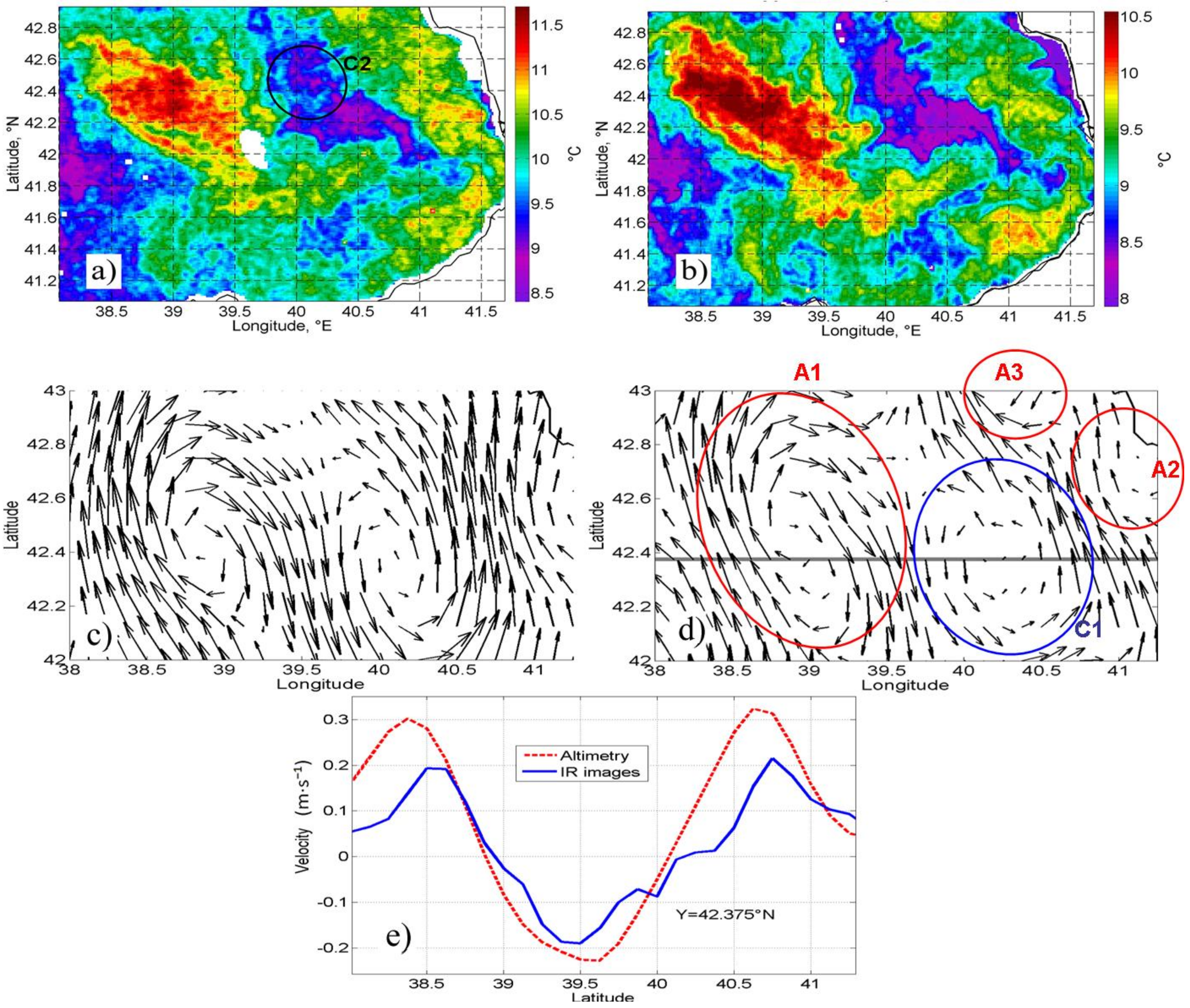
3.3. Scene 3: Cyclone–Anticyclone Pair in the Southeast Black Sea

Scene 3 demonstrates double eddy system observed in the eastern part of the Black Sea on 11 January 2007. It consisted of a warm anticyclone A1 (with SST~11°) and a colder cyclonic eddy C1 (SST~8°) with radiuses about 100 km (Figure 3a,b). Both the cyclone and anticyclone were oriented in the northwest–southeast direction, corresponding to the Rim current direction in this area. Currents computed from the satellite imagery represented well the dynamic structure of this system (Figure 3c,d), and it was also clearly defined by altimetry measurements. Both methods show that the radius of these eddies was about 60 km and the orbital velocity reached 0.2–0.3 m·s⁻¹ (Figure 3e).

However, velocity values were smaller in imagery-derived currents, particularly in the north and central parts of cyclonic eddy C1. This eddy is well manifested and smooth in altimetry data, but has a more complex structure in the satellite imagery. From the AVVHR imagery in Figure 3a we see on the north of eddy C1 one more small sub-mesoscale cyclonic eddy C2 (Figure 3a), which advects the warm water from the north. Its radius is only about 15 km and it cannot be appropriate resolved by altimetry measurements. The superposition of large cyclone C1 and small cyclone C2 may result in the complex structure of the current velocity derived from satellite imagery in Figure 3d.

Noticeable differences are observed between two velocity fields in Figure 3c,d along the eastern coast. Particularly, according to satellite imagery, the current flowing northward forms two anticyclonic meanders, A2 and A3 near the eastern coast with a radius of ~10–15 km (Figure 3d). Meander A2 in altimetry data is less pronounced. Altimetry data cannot appropriately describe the second coastal anticyclonic meander (A3), and altimetry-derived currents are directed to the north, perpendicular to the coast, without rotation at this part of the scene (Figure 3c). The inability of altimetry data to describe coastal eddy dynamics is observed also, more clearly, in Section 3.6. This is related, probably, to the absence of altimetry measurements near the coast, and the resulting inaccuracy of the mapping procedure, which leads to the formation of smooth maximums/minimums of dynamic topography and related smooth eddy fields. Another important reason is the inaccuracy of geophysical corrections, especially the mean dynamic topography in the coastal zone. At the same time, the anticyclonic eddy situated offshore is well represented by both methods, and estimates of velocities reasonably coincide.

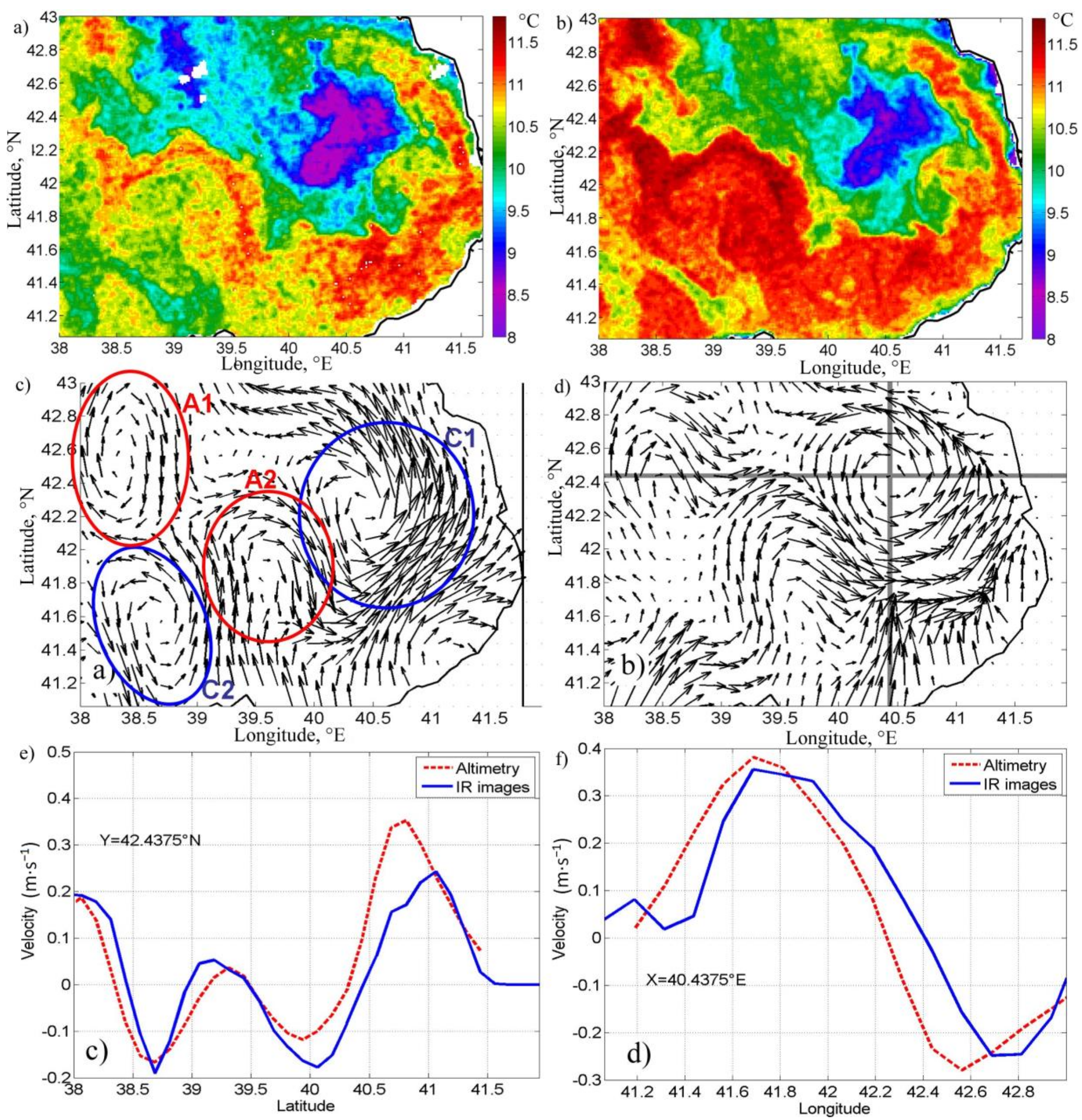
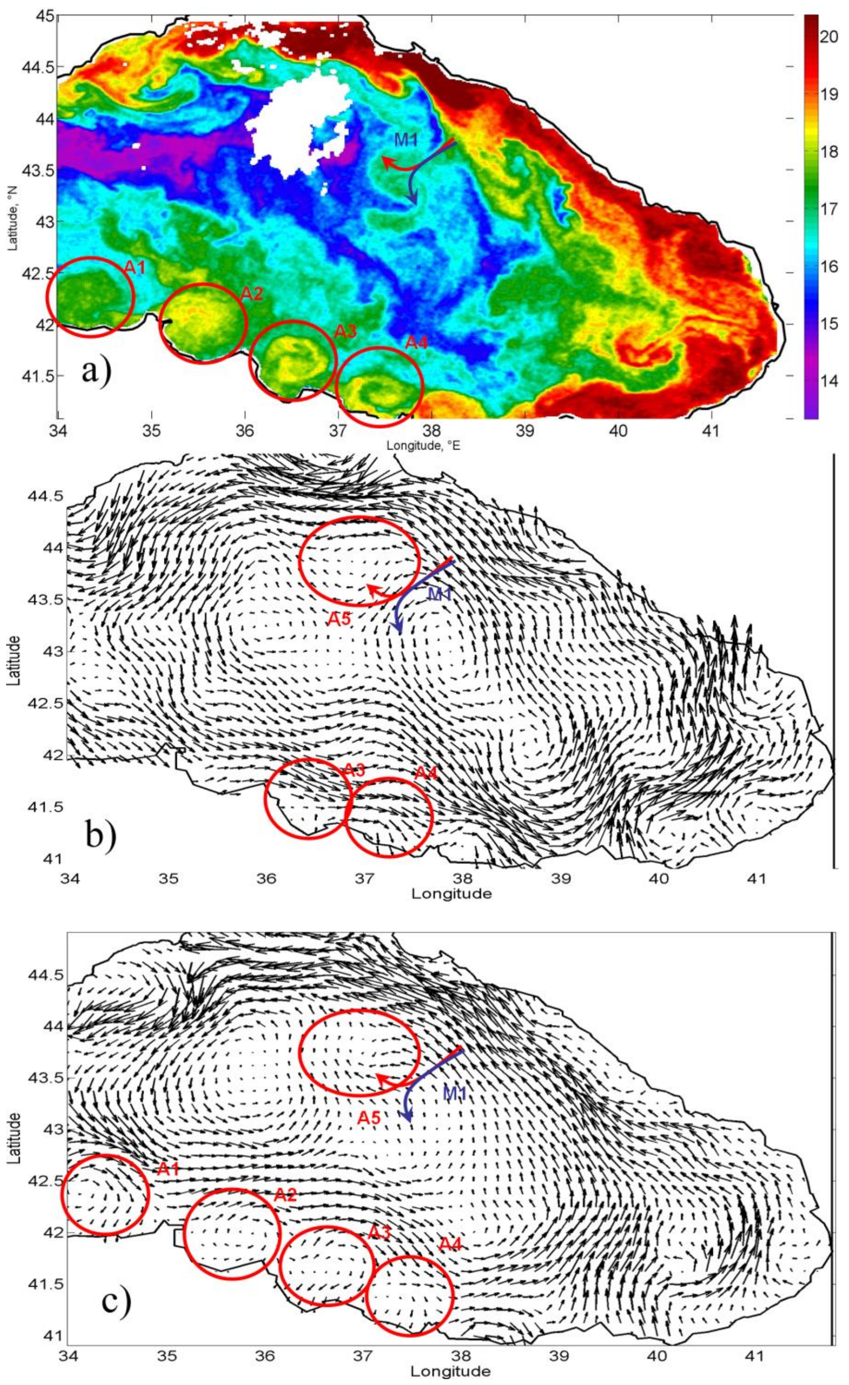
3.4. Scene 4: System of Eddies in the Southeastern Black Sea

The forth scene (Figure 4) represents the complex mesoscale dynamics in the southeastern Black Sea on 13 January 2005. Strong cyclonic eddy C1 with radius of 50 km is observed in the southeast of the scene. This cyclone with a relatively cold temperature in the core (~8°) is surrounded by warm coastal water (SST~11°). Interestingly, it is situated in the so-called Batumi anticyclone zone. Recent studies based on satellite altimetry [23,76] have shown that in contrast to the summer situation, when powerful anticyclones are often observed here, in winter strong cyclones are formed in this zone.

Some more mesoscale features are observed on the SST map: anticyclonic movement in the northeast (A1) and south (A2) of the map and a cyclonic eddy in the southwest (C2) (Figure 4a,b). Reconstructed maps of the velocity show all the abovementioned features of circulation (Figure 4c,d). The structure of the velocity field, positions, and values of maximums and minimums of the current velocity components computed from the two methods in Figure 4d coincide well (Figure 4c–f). However, eddies are more clearly pronounced in altimetry data. For example, eddy A1 has a distinct circular shape in the altimetry data, while in imagery-derived velocity it looks like an anticyclonic meander. The same is observed for eddies A2 and C2 in the south part of the scene. In the western part of the scene, velocities derived from 4D-Var look smoother and their magnitudes are generally smaller (Figure 4e). A possible reason for these discrepancies is the low contrast in satellite images in the east and south parts of the scene, where SST varies only ~1° from 10 °C to 11 °C. Uncertainties of current velocities during the low thermal contrasts are one of the known limitations of the methods, based on satellite imagery.

3.5. Scene 5: Basin-Scale Circulation Examples—26 June 2007

The SST field for 26 June 2007 and the calculated basin-scale circulation in the east part of the Black Sea, derived from both satellite methods, are presented in Figure 5a,c,d. Both methods agree as to the spatial structure and magnitudes of the currents. The main feature of the Black Sea circulation- the large-scale Rim current encircling the Black Sea in the cyclonic direction along the continental slope was successfully reproduced by altimetry and satellite imagery. A mesoscale cyclone with a radius of ~40 km and a maximal orbital velocity of ~0.2 m·s⁻¹ is observed in the southeast Black Sea. Rim current splits into two branches near this cyclone, with the branch to the west of the cyclone being significantly wider compared to the narrower jet at its east part (Figure 5c,d).

Figure 5b shows the differences between current fields reconstructed from satellite imagery and altimetry data. It can be seen that the differences are negligible in almost the whole study area, and are generally less than 0.05 m·s⁻¹. The only exception is the northeast part, where the Rim current derived from AVHHR imagery is significantly narrower than in the altimetry data, resulting in negative values in Figure 5b. This difference is probably related to the absence of tracers in thermal imagery in the central part of the basin (Figure 5a). This scene corresponds to a summer period, when thermal contrasts are often minimal due to strong solar heating and a thin mixed layer. These effects complicate the reproduction of summer circulation by thermal imagery.

3.6. Scene 6: Basin-Scale Circulation Examples—19 October 2005

The second basin-scale example corresponds to 23–24 October 2005. Several dynamic features are clearly seen in the AVHHR thermal image for 24 October 2005, 00:19: Rim current jet over the continental slope characterized by increased SST (18°–21°) compared to the central part of the basin (13°–16°), and a series of warm coastal anticyclonic eddies (A1…A4) in the south part of the basin (Figure 6a). Such near-shore anticyclones are important elements of the Black Sea dynamics investigated in many previous studies [21,77,78,79,80,81]. Mushroom current M1 transferring warm coastal water offshore is observed in the northeast part of the basin (38°E, 43.5°N).

Both methods are able to reproduce the Rim current and complex dynamics in the southeast part of the basin, related to the interaction of the eddies and large-scale dynamics (Figure 6b,c). An offshore jet related to the mushroom current M1 in the east part of the basin is also seen in both velocity fields. This current is related to the anticyclonic movement (A5) observed to the right of the Rim current in the northeastern part of the basin.

However, near-shore anticyclones A1–A4, clearly seen in the SST data, are almost absent in the altimetry data (Figure 6b). In altimetry-derived velocities, only weak anticyclonic rotation is seen at their location. We can observe only the northern “half” of the eddies with strong eastward orbital velocities and a complete absence of the coastal southern part of the eddy movement with westward orbital velocities. Velocities on the east eddy periphery are directed perpendicularly to the coast and eddy streamlines are not closed. The uncertainty and unclosed contours of the altimetry-derived circulation are probably a result of the mapping procedure. Extrapolation of sea level in the absence of along-track measurements will lead to the appearance of unclosed maximums and minimums of the sea level and related errors when describing eddy dynamics near the coast.

At the same time, coastal anticyclonic eddies are clearly distinguished in the velocity fields obtained by 4D-Var from satellite imagery (Figure 6c). The eddies are also characterized by pronounced asymmetry: the eastward velocities on their north periphery are significantly higher than the westward velocity on their south periphery. This asymmetry is probably the result of the superposition of orbital velocities of AEs and large-scale Rim current flowing eastward along the south coast. On the offshore side of the AE, velocity directions in eddy and Rim current coincide and, thereby, increase, while on the coastal side they are opposite and the total current decreases. Nevertheless, near-shore anticyclones are clearly reproduced by the second method. Their size (radius ~20 km) and position coincide well with their manifestation in SST maps. These near-shore eddies are very important for the Black Sea’s ecosystem as they provide ventilation of coastal areas and horizontal exchange of nutrients. At the moment satellite altimetry cannot reproduce this important part of the Black Sea dynamics, while satellite imagery provides reasonable results for coastal circulation. Methods based on satellite imagery, such as 4D-var assimilation, can be used to quantify present errors in altimetry coastal data.

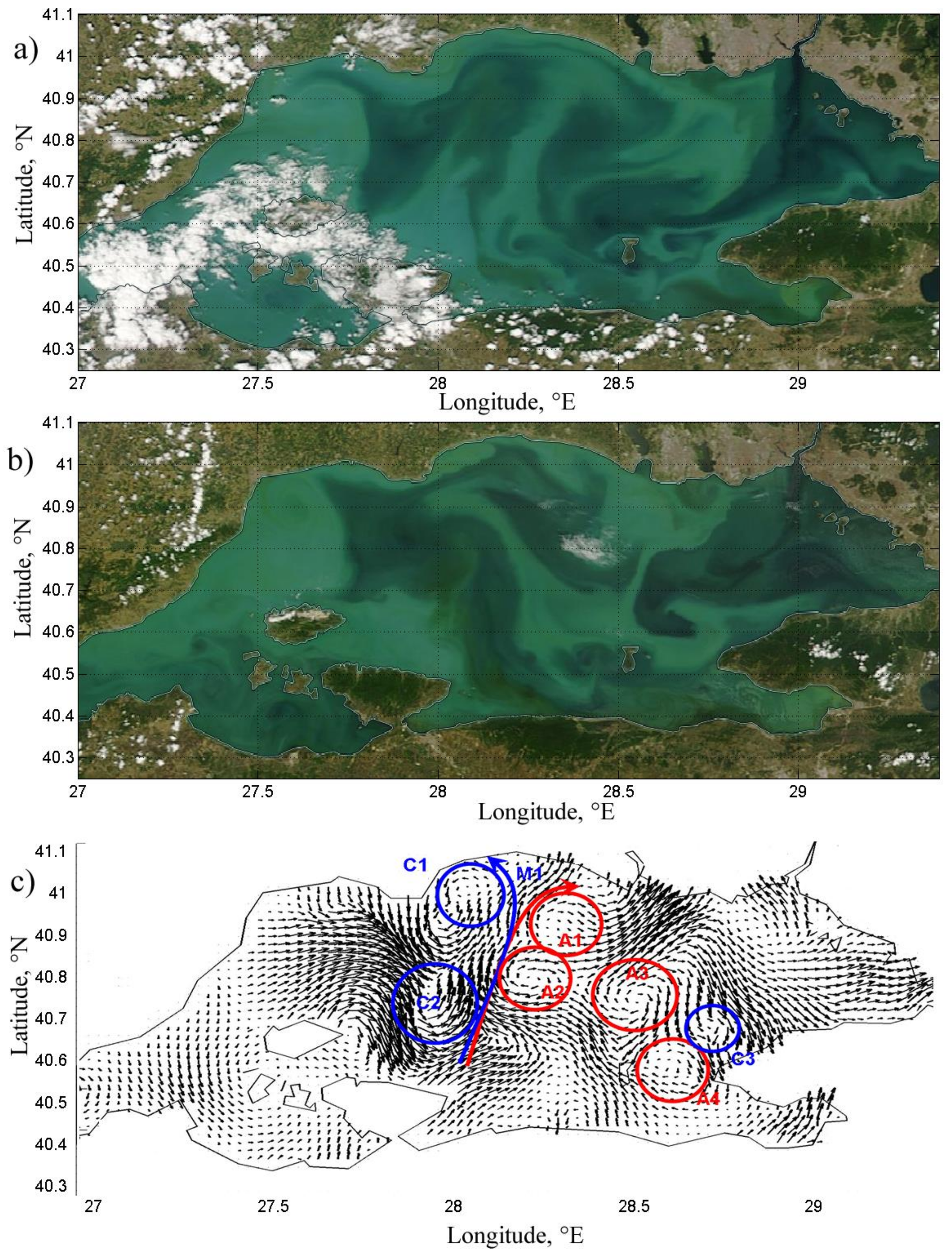
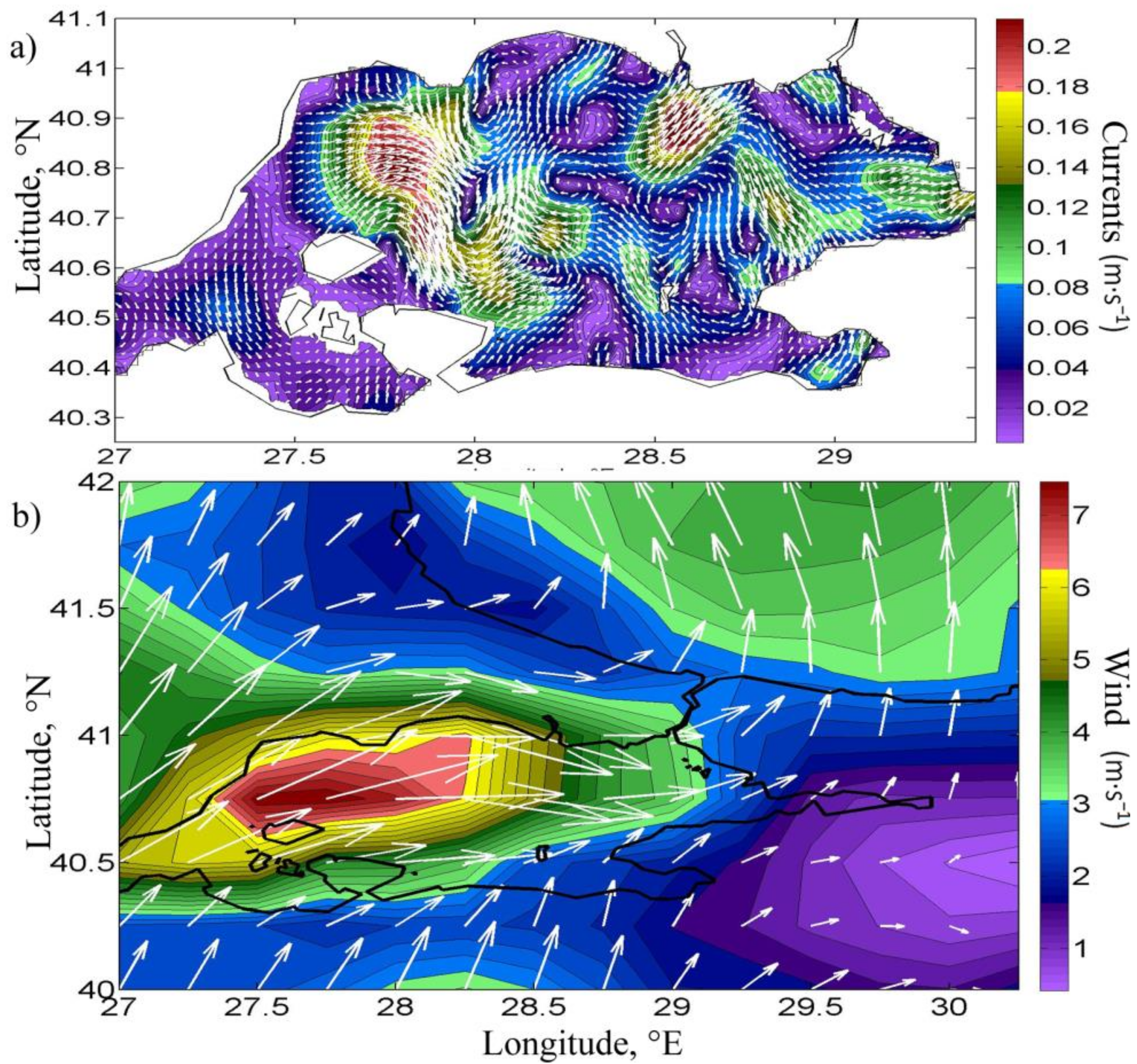
3.7. Reconstruction of the Marmara Sea Circulation

The Marmara Sea is the first link between the Black Sea and the Atlantic Ocean. Its dynamics plays a very important role in the interbasin exchange and inflow of the Mediterranean waters in the Black Sea [14,60,61,62,63,64]. On the other hand, the Black Sea dynamics significantly affect the Marmara Sea ecosystem and thermohaline variability [82]. However, due to the small geometrical size of the Marmara Sea (only 70 km in the meridional direction and ~150 km in the zonal direction) and the number of islands in the basin, the reconstruction of its dynamics is a challenging task for the satellite altimetry. In these conditions, the use of high-resolution imagery is one way to investigate the Marmara Sea circulation.

To demonstrate the efficiency of this method, we use MODIS-Aqua and MODIS-Terra 250-m resolution radiances at 0.62 µm–0.67 µm (https://ladsweb.modaps.eosdis.nasa.gov/). In order to use the 4D-Var method we took four consecutive images: MODIS-Aqua (25 and 26 May 2015) and MODIS-Terra (25 and 26 May 2015).

For visualization purposes, MODIS RGB composites (500 m resolution) obtained from Worldview portal (https://worldview.earthdata.nasa.gov/) are shown in Figure 7a,b. The complex dynamics of the basin, consisting of a series of eddies, mushroom currents, and jets, is clearly manifested in the optical tracers distribution (most probably coccolithophores). The reconstructed velocity field shows an intense mesoscale and sub-mesoscale dynamics that is in agreement with the satellite optical imagery (Figure 7c). At least six sub-mesoscale eddies are observed in the central part of the Marmara Sea. Two of them, A1 and C1, are situated at the end of intense mushroom current M1, which induces strong transport of matter across the whole basin from its south to its north part. This current is most intense at its south part (0.15 m·s⁻¹) and slows down to 0.08 m·s⁻¹near the north coast, where it splits into two eddies (Figure 8a). Eddies A1 and C1 have radiuses of only 8–10 km and a maximal orbital velocity of 0.05–0.1 m·s⁻¹. Two other eddies A2 and C2, which are smaller (radius only 5 km) but more intense (orbital velocity ~0.10–0.15 m·s⁻¹), are observed in the central part of the Marmara Sea on both sides of mushroom current M1.

Another series of eddies (A3, C2, and A4) is seen in the western part of the basin. In this part of the Marmara Sea the westward propagation of the dark Black Sea waters is seen in the optical imagery. It looks like a jet with decreased reflectance due to the absence of optical tracers (coccolithophores). This buoyant flow plays an important role in the Marmara Sea’s ecosystem [82]. On the end of this jet the formation of two eddies is observed: the relatively large A3 with radius of 8 km and orbital velocity of 0.05–0.10 m·s⁻¹; and small cyclone C3 with a radius less than 4 km and velocity 0.05–0.10 m·s⁻¹. Another relatively large anticyclone, A4, with radius ~5 km is observed between Imrali island and the East Turkish coast at ~(45°N, 28.7°E).

In the eastern and southern part of the sea, the currents are weakest and mainly directed to the east. The velocities obtained here are generally less than 0.04 m·s⁻¹. The most intense current velocities, which reach 0.25 m·s⁻¹, are observed in the northwestern part of the basin, above Marmara Island (Figure 8a). The intensification of eastward currents in this part of the basin is related to the wind forcing. At the time of measurement, the winds were eastward and had a local maximum in the northwest part of the basin with velocity up to 8 m·s⁻¹ (Figure 8b). The position and direction of the wind maximum coincide well with the maximum estimated current velocity. Therefore, the intensification of currents is mainly related to the wind drift currents. Wind drift currents play an important role in controlling fluxes across the Bosphorus and Dardanelles. Depending on the wind direction, they can lead to significant intensification or total blockage of the exchange across the straits [8,62,63]. Today, the relationship between wind and wind drift currents is still poorly understood, and the exact mechanisms of wind impact on the exchange in the strait are unknown. 4D-Var assimilation of satellite imagery can be used to provide new data on the relationship between atmospheric forcing and interbasin exchange.

Overall, we can conclude that the 4D-Var assimilation can be effectively used to study surface currents from large to submeso- spatial scales in small, enclosed basins, like the Marmara Sea, and can give valuable information about their dynamics.

4. Discussion

Satellite altimetry is an invaluable source of information about ocean dynamics. Many authors show the good quality of altimetry-derived geostrophic velocities all over the world. In the Black Sea, altimetry data were validated earlier using tide gauges, drifters, and hydrological data in a series of studies [6,7,8,9,10,11,12,13,14].

In our manuscript, we show that 4D-Var assimilation of satellite imagery provides results that coincide well with satellite altimetry during low wind conditions. This comparison with well-validated altimetry data instills confidence in the quality of the 4D-Var assimilation method. In coastal areas, mapped altimetry data is a source of several types of error related to uncertainties in atmospheric and geophysical corrections and extrapolation during mapping procedures with a deficiency of coastal along-track observations [26]. Methods based on satellite imagery, such as the 4D-Var used here [57], have no such disadvantages. Moreover, the coastal zone is often characterized by increased optical and thermal contrasts, which improves the accuracy of imagery-derived currents. That is why our results show that the spatial variability of coastal dynamics reconstructed from satellite imagery is more reasonable that altimetry-derived results. In particular, this is related to the reconstruction of coastal eddy dynamics, such as Black Sea nearshore anticyclones. These anticyclones are very important for the Black Sea basin, as they play an important role in the cross-shelf exchange of water masses and nutrients. Often, current streamlines in these eddies are not closed near the coast in altimetry data, which we relate, first, to the extrapolation during mapping procedure in the absence of coastal along-track data. These errors can strongly affect the estimates of the alongshore transport near the coast from altimetry data. Coastal currents computed from satellite imagery can be effectively used to quantify uncertainties and improve estimates of geophysical corrections for coastal altimetry data, e.g., mean dynamic topography, dynamic atmosphere correction, which is one of the tasks of modern remote sensing.

One of the factors that complicate such analysis is the impact of wind drift currents on the position of thermal fronts. In our study we observe that winds directly impact on the displacement of the thermal fronts in satellite imagery, causing disturbances that cannot be explained by geostrophic currents. It can be expected that the difference between altimetry-derived geostrophic velocity and (wind-driven + geostrophic) currents obtained from satellite imagery can give information on wind-driven currents in the surface layers for understanding its relationship with wind forcing [31,36]. This information is also very valuable as wind drift currents are important for many oceanographic tasks: e.g., for oil spill tracking, study of river plume dynamics, or interpretation of coastal radar data [83,84].

It should be noted that, in several cases, satellite imagery can underestimate current velocities. This is often observed in offshore areas and is related to the absence of pronounced contrast in satellite imagery. The necessity of manually controlling the quality of images in the presence of contrasts is one of the major disadvantages of the method. It significantly complicates the usage of satellite imagery for current computation on a regular basis. Another reason for current smoothing and underestimation is the use of regularization terms, which minimizes the gradient and divergence of current velocity during 4D-Var assimilation [57]. Parameters α, β of regularization can be manually decreased to minimize smoothing. However, usage of the data without smoothing can result in the appearance of spurious outliers in current velocity. The necessity to fit parameters α, β in certain cases is another weakness of the 4D-Var assimilation of satellite imagery, interfering with its usage in automatic mode.

5. Conclusions

Two different methods based on spaceborne measurements, satellite altimetry sea level measurements and 4D-Var analysis of IR image series, were used for surface current computation in the Black Sea basin. Results were compared for six different scenes with large-scale and mesoscale dynamic features. Both methods show their effectiveness in the determination of circulation in the Black Sea, such as for mesoscale eddies and jet currents. Reconstructed current fields are very close in terms of both amplitude and structure.

In coastal areas the quality of altimetry data decreases, while imagery-based methods have no such limitations and are expected to work better due to the strong thermal/optical contrasts in the coastal zone. This advantage of imagery-based velocities makes it possible to use them for the reconstruction of the dynamics of small, enclosed basins or lakes, or basins with many islands. The current computation methods based on satellite imagery have the possibility of reconstructing ocean dynamics with significantly higher resolution than altimetry does. They can be very valuable for the analysis of small basin dynamics and common sub-mesoscale dynamics in the ocean. In our study we use 4D-Var assimilation of 250 m Modis imagery to describe the currents in the Marmara Sea, whose circulation is still poorly known. The results show the complex dynamics of the basin, including several intense mesoscale and sub-mesoscale eddies.

The evaluation of current velocities from satellite image series will be extremely valuable for oceanography, considering the rising amount of high-resolution optical and infrared data. The usage of consecutive images of freely available LandSat 7/8, Sentinel 2 would allow us to reconstruct sub-mesoscale velocity fields on the scale of several hundred meters to take our understanding of ocean dynamics to the next level.

References

1. Nerem, R.S.; Schrama, E.J.; Koblinsky, C.J.; Beckley, B.D. A preliminary evaluation of ocean topography from the TOPEX/POSEIDON mission. J. Geophys. Res. Oceans 1994, 99, 24565–24583. [Google Scholar] [CrossRef]
2. Fu, L.-L.; Cazenave, A. Satellite Altimetry and Earth Sciences: A Handbook of Techniques and Applications; International Geophysics Series; Academic Press: London, UK, 2001; Volume 69, p. 463. [Google Scholar]
3. Fu, L.L.; Le Traon, P. Satellite altimetry and ocean dynamics. Comptes Rendus Geosci. 2006, 338, 1063–1076. [Google Scholar] [CrossRef]
4. Xu, Y.; Li, J.; Dong, S. Ocean circulation from satellite altimetry: Progresses and challenges. In Ocean Circulation and El Nino; Long, J.A., Wells, D.S., Eds.; Nova Science Publishers, Inc.: New York, NY, USA, 2009; ISBN 978-1-60692-084-8. [Google Scholar]
5. Morrow, R.; Le Traon, P.Y. Recent advances in observing mesoscale ocean dynamics with satellite altimetry. Adv. Space Res. 2012, 50, 1062–1076. [Google Scholar] [CrossRef]
6. Korotaev, G.K.; Saenko, O.A.; Koblinsky, C.J.; Demishev, S.G.; Knysh, V.V. An accuracy, methodology, and some results of the assimilation of the TOPEX/Poseidon altimetry data into the model of the Black Sea general circulation. Earth Res. Space 1998, 3, 3–17. [Google Scholar]
7. Stanev, E.V.; Le Traon, P.Y.; Peneva, E.L. Sea level variations and their dependency on meteorological and hydrological forcing: Analysis of altimeter and surface data for the Black Sea. J. Geophys. Res.-Oceans 2000, 105, 17203–17216. [Google Scholar] [CrossRef]
8. Stanev, E.V.; Peneva, E.L. Regional sea level response to global climatic change: Black Sea examples. Glob. Planet. Chang. 2001, 32, 33–47. [Google Scholar] [CrossRef]
9. Goryachkin, Y.N.; Ivanov, V.A.; Lemeshko, E.M.; Lipchenko, M.M. Application of the altimetry data to the analysis of water balance of the Black Sea. Phys. Oceanogr. 2003, 13, 355–360. [Google Scholar] [CrossRef]
10. Kubryakov, A.A.; Stanichny, S.V. Estimating the Quality of the Retrieval of the Surface Geostrophic Circulation of the Black Sea by Satellite Altimetry Data Based on Validation with Drifting Buoy Measurements Izvestiya. Atmos. Ocean. Phys. 2013, 49, 930–938. [Google Scholar] [CrossRef]
11. Kubryakov, A.A.; Stanichnyi, S.V. The Black Sea level trends from tide gages and satellite altimetry. Russ. Meteorol. Hydrol. 2013, 38, 329–333. [Google Scholar] [CrossRef]
12. Kubryakov, A.A.; Stanichny, S.V.; Zatsepin, A.G.; Kremenetskiy, V.V. Long-term variations of the Black Sea dynamics and their impact on the marine ecosystem. J. Mar. Syst. 2016, 163, 80–94. [Google Scholar] [CrossRef]
13. Avsar, N.B.; Jin, S.; Kutoglu, H.; Gurbuz, G. Sea level change along the Black Sea coast from satellite altimetry, tide gauge and GPS observations. Geod. Geodyn. 2016, 7, 50–55. [Google Scholar] [CrossRef]
14. Volkov, D.L.; Landerer, F.W. Internal and external forcing of sea level variability in the Black Sea. Clim. Dyn. 2015, 45, 2633–2646. [Google Scholar] [CrossRef]
15. Korotaev, G.K.; Saenko, O.A.; Koblinsky, C.J. Satellite altimetry observations of the Black Sea level. J. Geophys. Res. 2001, 106, 917–933. [Google Scholar] [CrossRef]
16. Sokolova, E.; Stanev, E.V.; Yakubenko, V.; Ovchinnikov, I.; Kos’yan, R. Synoptic variability in the Black Sea. Analysis of hydrographic survey and altimeter data. J. Mar. Syst. 2001, 31, 45–63. [Google Scholar] [CrossRef]
17. Korotaev, G.; Oguz, T.; Nikiforov, A.; Koblinsky, C. Seasonal, interannual, and mesoscale variability of the Black Sea upper layer circulation derived from altimeter data. J. Geophys. Res. 2003, 108, 3122. [Google Scholar] [CrossRef]
18. Kubryakov, A.A.; Stanichny, S.V. Mesoscale eddies in the Black Sea from satellite altimetry data. Oceanology 2015, 55, 56–67. [Google Scholar] [CrossRef]
19. Kubryakov, A.A.; Stanichny, S.V. Seasonal and interannual variability of the Black Sea eddies and its dependence on characteristics of the large-scale circulation. Deep Sea Res. Part I Oceanogr. Res. Pap. 2015, 97, 80–91. [Google Scholar] [CrossRef]
20. Grayek, S.; Stanev, E.V.; Kandilarov, R. On the response of Black Sea level to external forcing: Altimeter data and numerical modelling. Ocean Dyn. 2010, 60, 123–140. [Google Scholar] [CrossRef]
21. Zatsepin, A.G.; Ginzburg, A.I.; Kostianoy, A.G.; Kremenetskiy, V.V.; Krivosheya, V.G.; Stanichny, S.V.; Poulain, P.M. Observations of Black Sea mesoscale eddies and associated horizontal mixing. J. Geophys. Res. Oceans 2003, 108, 3246. [Google Scholar] [CrossRef]
22. Shapiro, G.I.; Stanichny, S.V.; Stanychna, R.R. Anatomy of shelf—Deep sea exchanges by a mesoscale eddy in the North West Black Sea as derived from remotely sensed data. Remote Sens. Environ. 2010, 114, 867–875. [Google Scholar] [CrossRef]
23. Menna, M.; Poulain, P.M. Geostrophic currents and kinetic energies in the Black Sea estimated from merged drifter and satellite altimetry data. Ocean Sci. 2014, 10, 155–165. [Google Scholar] [CrossRef] [Green Version]
24. Le Traon, P.-Y.; Dibarboure, G.; Ducet, N. Use of a High-Resolution Model to Analyze the Mapping Capabilities of Multiple-Altimeter Missions. J. Atmos. Ocean. Technol. 2001, 18, 1277–1288. [Google Scholar] [CrossRef]
25. Pascual, A.; Faugere, Y.; Larnicol, G.; Le Traon, P.-Y. Improved description of the ocean mesoscale variability by combining four satellite altimeters. Geophys. Res. Lett. 2006, 33. [Google Scholar] [CrossRef]
26. Vignudelli, S.; Kostianoy, A.G.; Cipollini, P.; Benveniste, J. (Eds.) Coastal Altimetry; Springer Science Business Media: Berlin, Germany, 2011. [Google Scholar]
27. Desportes, C.; Obligis, E.; Eymard, L. On the wet tropospheric correction for altimetry in coastal regions. IEEE Trans. Geosci. Remote Sens. 2007, 45, 2139–2149. [Google Scholar] [CrossRef]
28. Volkov, D.L.; Larnicol, G.; Dorandeu, J. Improving the quality of satellite altimetry data over continental shelves. J. Geophys. Res. Oceans 2007, 112. [Google Scholar] [CrossRef]
29. Dohan, K.; Maximenko, N. Monitoring ocean currents with satellite sensors. Oceanography 2010, 23, 94–103. [Google Scholar] [CrossRef]
30. Marcos, M.; Pascual, A.; Pujol, I. Improved satellite altimeter mapped sea level anomalies in the Mediterranean Sea: A comparison with tide gauges. Adv. Space Res. 2015, 56, 596–604. [Google Scholar] [CrossRef]
31. Liu, Y.; Weisberg, R.H.; Vignudelli, S.; Roblou, L.; Merz, C.R. Comparison of the X-TRACK altimetry estimated currents with moored ADCP and HF radar observations on the West Florida Shelf. Adv. Space Res. 2012, 50, 1085–1098. [Google Scholar] [CrossRef]
32. Bonjean, F.; Lagerloef, G.S. Diagnostic model and analysis of the surface currents in the tropical Pacific Ocean. J. Phys. Oceanogr. 2002, 32, 2938–2954. [Google Scholar] [CrossRef]
33. Poulain, P.M.; Gerin, R.; Mauri, E.; Pennel, R. Wind effects on drogued and undrogued drifters in the Eastern Mediterranean. J. Atmos. Ocean. Technol. 2009, 26, 1144–1156. [Google Scholar] [CrossRef]
34. Stanichny, S.V.; Kubryakov, A.A.; Soloviev, D.M. Parameterization of surface wind-driven currents in the Black Sea using drifters, wind, and altimetry data. Ocean Dyn. 2016, 66, 1–10. [Google Scholar] [CrossRef]
35. Issa, L.; Brajard, J.; Fakhri, M.; Hayes, D.; Mortier, L.; Poulain, P.M. Modelling surface currents in the Eastern Levantine Mediterranean using surface drifters and satellite altimetry. Ocean Model. 2016, 104, 1–14. [Google Scholar] [CrossRef] [Green Version]
36. Liu, Y.; Weisberg, R.H.; Vignudelli, S.; Mitchum, G.T. Evaluation of altimetry derived surface current products using Lagrangian drifter trajectories in the eastern Gulf of Mexico. J. Geophys. Res. Oceans 2014, 119, 1842–2827. [Google Scholar] [CrossRef]
37. Qazi, W.A.; Emery, W.J.; Fox-Kemper, B. Computing ocean surface currents over the coastal California current system using 30-min-lag sequential SAR images. IEEE Trans. Geosci. Remote Sens. 2014, 52, 7559–7580. [Google Scholar] [CrossRef]
38. Horn, B.K.; Schunck, B.G. Determining optical flow. Artif. Intell. 1981, 17, 185–203. [Google Scholar] [CrossRef]
39. Kelly, K.A. An inverse model for near-surface velocity from infrared images. J. Phys. Oceanogr. 1989, 19, 1845–1864. [Google Scholar] [CrossRef]
40. Kelly, K.A.; Strub, P.T. Comparison of Velocity Estimates from advanced very high resolution radiometer in the coastal transition zone. J. Geophys. Res. 1992, 97, 9653–9668. [Google Scholar] [CrossRef]
41. Vigan, X.; Provost, C.; Podesta, G. Sea surface velocities from sea surface temperature image sequences: 2. Application to the Brazil-Malvinas Confluence area. J. Geophys. Res. Oceans 2000, 105, 19515–19534. [Google Scholar] [CrossRef]
42. Corpetti, T.; Heitz, D.; Arroyo, G.; Memin, E.; Santa-Cruz, A. Fluid experimental flow estimation based on an optical-flow scheme. Exp. Fluids 2006, 40, 80–97. [Google Scholar] [CrossRef]
43. Chen, W. Surface velocity estimation from satellite imagery using displaced frame central difference equation. IEEE Trans. Geosci. Remote Sens. 2012, 50, 2791–2801. [Google Scholar] [CrossRef]
44. Leese, J.A.; Novak, C.S.; Clark, B.B. An automated technique for obtaining cloud motion from geosynchronous satellite data using cross correlation. J. Appl. Meteorol. 1971, 10, 118–132. [Google Scholar] [CrossRef]
45. Emery, W.J.; Thomas, A.C.; Collins, M.J.; Crawford, W.R.; Mackas, D.L. An objective method for computing advective surface velocities from sequential infrared satellite images. J. Geophys. Res. Oceans 1986, 91, 12865–12878. [Google Scholar] [CrossRef]
46. Afanasyev, Y.D.; Kostianoy, A.G.; Zatsepin, A.G.; Poulain, P.M. Analysis of velocity field in the eastern Black Sea from satellite data during the Black Sea’99 experiment. J. Geophys. Res. Oceans 2002, 107. [Google Scholar] [CrossRef]
47. Bowen, M.M.; Emery, W.J.; Wilkin, J.L.; Tildesley, P.C.; Barton, I.J.; Knewtson, R. Extracting multiyear surface currents from sequential thermal imagery using the maximum cross-correlation technique. J. Atmos. Ocean. Technol. 2002, 19, 1665–1676. [Google Scholar] [CrossRef]
48. Zavialov, P.O.; Grigorieva, J.V.; Möller, O.O.; Kostianoy, A.G., Jr.; Gregoire, M. Continuity preserving modified maximum cross-correlation technique. J. Geophys. Res. Oceans 2002, 107, 3160. [Google Scholar] [CrossRef]
49. Crocker, R.I.; Matthews, D.K.; Emery, W.J.; Baldwin, D.G. Computing coastal ocean surface currents from infrared and ocean color satellite imagery. IEEE Trans. Geosci. Remote Sens. 2007, 45, 435–447. [Google Scholar] [CrossRef]
50. Notarstefano, G.; Poulain, P.M.; Mauri, E. Estimation of surface currents in the Adriatic Sea from sequential infrared satellite images. J. Atmos. Ocean. Technol. 2008, 25, 271–285. [Google Scholar] [CrossRef]
51. Matthews, D.K.; Emery, W.J. Velocity observations of the California Current derived from satellite imagery. J. Geophys. Res. Oceans 2009, 114. [Google Scholar] [CrossRef]
52. Yang, H.; Arnone, R.; Jolliff, J. Estimating advective near-surface currents from ocean color satellite images. Remote Sens. Environ. 2015, 158, 1–14. [Google Scholar] [CrossRef]
53. Heuzé, C.; Carvajal, G.K.; Eriksson, L.E.; Soja-Woźniak, M. Sea Surface Currents Estimated from Spaceborne Infrared Images Validated against Reanalysis Data and Drifters in the Mediterranean Sea. Remote Sens. 2017, 9, 422. [Google Scholar] [CrossRef]
54. Liu, J.; Emery, W.J.; Wu, X.; Li, M.; Li, C.; Zhang, L. Computing Coastal Ocean Surface Currents from MODIS and VIIRS Satellite Imagery. Remote Sens. 2017, 9, 1083. [Google Scholar] [CrossRef]
55. Bruhn, A.; Weickert, J.; Schnörr, C. Lucas/Kanade Meets Horn/Schunck: Combining Local and Global Optic Flow Methods. Int. J. Comput. Vis. 2005, 61, 211. [Google Scholar] [CrossRef]
56. Babiy, V.I.; Pogrebnoy, A.E.; Ratner, Y.B.; Stanichny, S.V. Possibilities of the reconstruction of surface currents velocity field from satellite data (on the example of the Black Sea). In Environamental Monitoring Systems; NASU MHI: Sevastopol, Ukraine, 2002; ISBN 966-02-2491-5. [Google Scholar]
57. Korotaev, G.K.; Huot, E.; Le Dimet, F.X.; Herlin, I.; Stanichny, S.V.; Solovyev, D.M.; Wu, L. Retrieving ocean surface current by 4-D variational assimilation of sea surface temperature images. Remote Sens. Environ. 2008, 112, 1464–1475. [Google Scholar] [CrossRef]
58. Huot, E.; Herlin, I.; Mercier, N.; Plotnikov, E.V. (2010, August). Estimating apparent motion on satellite acquisitions with a physical dynamic model. In Proceedings of the 2010 20th International Conference on Pattern Recognition (ICPR), Istanbul, Turkey, 23–26 August 2010; pp. 41–44. [Google Scholar]
59. Chen, W. Nonlinear inverse model for velocity estimation from an image sequence. J. Geophys. Res. Oceans 2011, 116. [Google Scholar] [CrossRef]
60. Beşiktepe, Ş.T.; Sur, H.I.; Özsoy, E.; Latif, M.A.; Oǧuz, T.; Ünlüata, Ü. The circulation and hydrography of the Marmara Sea. Prog. Oceanogr. 1994, 34, 285–334. [Google Scholar] [CrossRef]
61. Aksu, A.E.; Hiscott, R.N.; Yaşar, D. Oscillating Quaternary water levels of the Marmara Sea and vigorous outflow into the Aegean Sea from the Marmara Sea–Black Sea drainage corridor. Mar. Geol. 1999, 153, 275–302. [Google Scholar] [CrossRef]
62. Gregg, M.C.; Özsoy, E. Flow, water mass changes, and hydraulics in the Bosphorus. J. Geophys. Res. Oceans 2002, 107. [Google Scholar] [CrossRef]
63. Jarosz, E.; Teague, W.J.; Book, J.W.; Beşiktepe, Ş. On flow variability in the Bosphorus Strait. J. Geophys. Res. Oceans 2011, 116. [Google Scholar] [CrossRef]
64. Stanev, E.V.; Grashorn, S.; Zhang, Y.J. Cascading ocean basins: Numerical simulations of the circulation and interbasin exchange in the Azov-Black-Marmara-Mediterranean Seas system. Ocean Dyn. 2017, 67, 1003–1025. [Google Scholar] [CrossRef]
65. Chelton, D.B.; Ries, J.C.; Haines, B.J.; Fu, L.L.; Callahan, P.S. Satellite altimetry. Int. Geophys. 2001, 69, 1-ii. [Google Scholar]
66. Cheney, R.; Miller, L.; Agreen, R.; Doyle, N.; Lillibridge, J. Topex/Poseidon: The 2-cm solution. J. Geophys. Res. Oceans 1994, 99, 24555–24563. [Google Scholar] [CrossRef]
67. Rio, M.H.; Hernandez, F. A mean dynamic topography computed over the world ocean from altimetry, in situ measurements, and a geoid model. J. Geophys. Res. Oceans 2004, 109. [Google Scholar] [CrossRef]
68. Maximenko, N.; Niiler, P.; Centurioni, L.; Rio, M.H.; Melnichenko, O.; Chambers, D.; Galperin, B. Mean dynamic topography of the ocean derived from satellite and drifting buoy data using three different techniques. J. Atmos. Ocean. Technol. 2009, 26, 1910–1919. [Google Scholar] [CrossRef]
69. Kubryakov, A.A.; Stanichny, S.V. Mean Dynamic Topography of the Black Sea, computed from altimetry, drifter measurements and hydrology data. Ocean Sci. 2011, 7, 745–753. [Google Scholar] [CrossRef]
70. Rio, M.H.; Guinehut, S.; Larnicol, G. New CNES-CLS09 global mean dynamic topography computed from the combination of GRACE data, altimetry, and in situ measurements. J. Geophys. Res. Oceans 2011, 116. [Google Scholar] [CrossRef]
71. Chelton, D.B.; Schlax, M.G.; Samelson, R.M. Global observations of nonlinear mesoscale eddies. Prog. Oceanogr. 2011, 91, 167–216. [Google Scholar] [CrossRef]
72. Arakawa, A.; Lamb, V.R. Computational design of the basic dynamical processes of the UCLA general circulation model. Methods Comput. Phys. 1977, 17, 173–265. [Google Scholar]
73. Gilbert, J.-C.; Lemaréchal, C. The Modules M1QN3 and N1QN3; Version 2.0c. Tech. Rep.; INRIA: Paris, France, 1995.
74. Plotnikov, E.V. Cloud filtration technique for the Black-Sea AVHRR data. Phys. Oceanogr. 2009, 19, 186–196. [Google Scholar] [CrossRef]
75. Rienecker, M.M.; Suarez, M.J.; Gelaro, R.; Todling, R.; Bacmeister, J.; Liu, E.; Bloom, S. MERRA: NASA’s modern-era retrospective analysis for research and applications. J. Clim. 2011, 24, 3624–3648. [Google Scholar] [CrossRef]
76. Kubryakov, A.; Stanichny, S. Dynamics of Batumi Anticyclone from the Satellite Measurements. Phys. Oceanogr. 2015, 2, 59–68. [Google Scholar]
77. Ivanov, V.A.; Belokopytov, V.N. Oceanography of the Black Sea; ECOSY-Gidrofizika; National Academy of Sciences of Ukraine, Marine Hydrophysical Institute: Sevastopol, Ukraine, 2013; p. 210. ISBN 978-966-022-6165-5. [Google Scholar]
78. Oguz, T.; Latun, V.S.; Latif, M.A.; Vladimirov, V.V.; Sur, H.I.; Markov, A.A.; Ünlüata, Ü. Circulation in the surface and intermediate layers of the Black Sea. Deep Sea Res. Part I Oceanogr. Res. Pap. 1993, 40, 1597–1612. [Google Scholar] [CrossRef]
79. Krivosheya, V.G.; Ovchinnikov, I.M.; Titov, V.B.; Yakubenko, V.G.; Skirta, A.Y. Meandering of the Main Black Sea Current and eddies formation in the north-eastern part of the Black Sea in summer 1994. Okeanologiya 1998, 38, 546–553. [Google Scholar]
80. Ginzburg, A.I.; Kostianoy, A.G.; Krivosheya, V.G.; Nezlin, N.P.; Soloviev, D.M.; Stanichny, S.V.; Yakubenko, V.G. Mesoscale eddies and related processes in the northeastern Black Sea. J. Mar. Syst. 2002, 32, 71–90. [Google Scholar] [CrossRef]
81. Karimova, S. Eddy statistics for the Black Sea by visible and infrared remote sensing. In Remote Sensing of the Changing Oceans; Springer: Berlin/Heidelberg, Germany, 2011; pp. 61–75. [Google Scholar]
82. Oguz, T. Impacts of a buoyant strait outflow on the plankton production characteristics of an adjacent semi-enclosed basin: A case study of the Marmara Sea. J. Mar. Syst. 2017, 173, 90–100. [Google Scholar] [CrossRef]
83. Abascal, A.J.; Castanedo, S.; Mendez, F.J.; Medina, R.; Losada, I.J. Calibration of a Lagrangian transport model using drifting buoys deployed during the Prestige oil spill. J. Coas. Res. 2009, 25, 80–90. [Google Scholar] [CrossRef]
84. Kubryakov, A.A.; Stanichny, S.V.; Zatsepin, A.G. Interannual variability of Danube waters propagation in summer period of 1992–2015 and its influence on the Black Sea ecosystem. J. Mar. Syst. 2018, 179, 10–30. [Google Scholar] [CrossRef]
Figure 1. (ac) AVHHR SST in the vicinity of the Sevastopol anticyclone on 13 May 2005 09:11 (a), 13 May 2005 13:55 (b), 14 May 2005 00:34 (c); (d,e) Surface current calculated for 13 May 2005 from altimetry (d), from IR images (solid line—sections) (e); (f,g) meridional section of u (f), zonal section of v (g) (red line—altimetry; blue—IR images).
Remotesensing 10 00239 g001
Figure 2. (a,b) AVHHR SST at 13 February 2007 23:15 (a); 14 February 2007 08:36 (b); (c) Wind velocity from Merra dataset at 14 February 2007 06:00; (d,e) Surface current calculated for 13 February 2007 from altimetry (d), from IR images (solid line—sections) (e); (f,g) meridional section of u (f), zonal section of v (g) (red—altimetry; blue—IR images).
Remotesensing 10 00239 g002
Figure 3. (a,b) AVHHR SST at 11 January 2007 19:40 (a), 12 January 2007 07:56 (b); (c,d) Surface current calculated for 12 January 2007 from altimetry (c), from IR images (solid line—section) (d); (e) meridional section of u (red line—altimetry; blue—IR images).
Remotesensing 10 00239 g003
Figure 4. (a,b) AVHHR SST at 13 January 2005 08:13 (a); 13 Jan 2005 14:49 (b); (c,d) Surface current calculated for 13 January 2005 from altimetry (c), from IR images (solid line—sections) (d); (e,f) meridional section of u (e), zonal section of v (f) (red line—altimetry; blue—IR images).
Remotesensing 10 00239 g004
Figure 5. AVHHR SST at 26 June 2007 19:12 (a); Difference between currents calculated from IR imagery and altimetry data (b); surface currents calculated for 27 June 2007 from altimetry data (c) and IR images (d).
Remotesensing 10 00239 g005
Figure 6. (a) AVHHR SST at 24 October 2005 00:19; (b) surface current calculated from altimetry; (c) surface current calculated from AVHHR imagery using 4D-Var.
Remotesensing 10 00239 g006
Figure 7. (a) MODIS-Aqua RGB composite at 25 May 2015 9:00; (b) MODIS-Terra RGB composite at 26 May 2015, 11:25; (c) current velocity calculated from optical imagery using 4D-Var.
Remotesensing 10 00239 g007
Figure 8. (a) Current magnitude (m·s−1) computed from 4D-Var assimilation of Modis imagery; (b) wind velocity over the Marmara Sea on 25 May 2015 18:00 UTC.
Remotesensing 10 00239 g008