Satellite and In Situ Observations for Advancing Global Earth Surface Modelling: A Review

 ,
,  ,
,  , ,
, ,  , ,
, ,  , ,
, ,  ,
,  ,
,  ,
,  , , , , , , , ,
  , , add
Show full author list
, , add
Show full author list
Abstract
1. Introduction
2. EO Satellite and In Situ Observations for Earth Surface
2.1. SMOS Soil Moisture Ocean Salinity Mission
2.2. SMAP Soil Moisture Active Passive Mission
2.3. TERRA/AQUA—MODIS
2.4. LANDSAT and Its Legacy
2.5. SEASAT and Its Legacy
2.6. Copernicus Sentinels
2.7. GOES, METEOSAT and Other Geostationary Satellites
2.8. Ground-Based Networks
2.9. Ocean-Based Networks
3. Earth Surface Modelling Advances and Links with EO Datasets
3.1. Land-Surface Reservoirs
- Enhanced realism of the representation of water and energy stocks in soil, snow and inland water bodies, via parameterisations and physiography revisions.
- Improved fluxes for land-atmosphere energy and water exchanges, inclusion of natural and anthropogenic carbon emissions, and improved river discharges.
3.1.1. Soil
3.1.2. Seasonal Snow Cover
3.1.3. Permanent Snow and Ice
3.1.4. Vegetation and Carbon Cycle
3.2. Land–Atmosphere Fluxes
3.2.1. CO2 Natural Ecosystem Exchange
3.2.2. CH4 Natural Methane Fluxes
3.2.3. Vegetation Water Fluxes
3.2.4. CO2 Anthropogenic Fluxes and Co-Emitters
3.3. Land Surface Properties
3.3.1. Orography
3.3.2. Soil Depth
3.3.3. Soil Texture
3.4. Inland-Waters
3.5. River Discharge and Hydrological Forecasting
3.6. Land–Atmosphere Coupling
3.7. Ocean–Atmosphere Coupling
3.8. Ocean Cryosphere: Snow and Ice
4. Towards Enhanced Global-Scale Local-Relevant Monitoring and Forecasting
4.1. Anthropogenic Surface Modifications
4.1.1. Urban Areas
4.1.2. Changing Water Bodies and Irrigated Areas
4.2. Relevance for Atmospheric Composition
4.3. Improved Diurnal Cycle for Assimilation Purposes
5. Towards Enhanced Use of High Resolution EO Data in Earth System Modelling
5.1. Towards More Comprehensive Model Improvement through Joint Use of Multivariate EO Data
5.2. Delivering EO-Driven Research to Services
5.3. Satellite-Focused Field Campaign: The Concordiasi Example
5.4. Links with the World Weather/Climate Research WWRP/WCRP Programmes
5.5. Links with EO Satellite Data Providers
5.6. An International Surface Working Group
6. Conclusions
- The improvement of parameterisation schemes over land and water surfaces to reduce systematic model errors that are clearly associated to missing processes (e.g., lack or spatial resolution in horizontal and vertical dimension, inadequate representation of local physiography) that impair the realism of surface fluxes partitioning.
- The development of observation operators that map the observed satellite radiance into physical quantities that are represented in models, particularly for thermal infrared imagers (e.g., for LST) and low-frequency microwave radiometer/radars (e.g., for L-band brightness temperature).
- The improvement of assimilation schemes capable of handling the models and observations uncertainties related to surface heterogeneities and processes and associated to the diverse remote sensing resolutions (e.g., LST and L-band). Data assimilation shall make use of observations for constraining both surface state-variables and fluxes.
Author Contributions
Funding
Acknowledgments
Conflicts of Interest
Abbreviations
| AIRS | Atmospheric InfraRed Sounder |
| AMSR-E | Advanced Microwave Scanning Radiometer for EOS (Earth Observing System) |
| AMSR-2 | Advanced Microwave Scanning Radiometer 2 |
| AMSU-A | Advanced Microwave Sounding Unit-A |
| AROME | Action de Recherche Petite Echelle Grande Echelle |
| ASTER | Advanced Spaceborne Thermal Emission and Reflection Radiometer |
| ATSR | Along Track Scanning Radiometers |
| AVHRR | Advanced Very High Resolution Radiometer |
| BEVAP | Bare-ground Evaporation |
| BSWB | Basin Scale Water Balance |
| C3S | Copernicus Climate Change Service |
| CALIPSO | Cloud-Aerosol Lidar and Infrared Pathfinder Satellite Observation |
| CAMS | Copernicus Atmosphere Monitoring Service |
| CASA | Carnegie–Ames–Stanford Approach |
| CEMS | Copernicus Emergency Monitoring Service |
| CERES | Clouds and the Earth’s Radiant Energy System |
| CGLS | Copernicus Global Land Service |
| CH-TESSEL | Carbon and Hydrology—Tiled ECMWF Scheme for Surface Exchanges over Land |
| CLM | Community Land Model |
| CMA | China Meteorological Agency |
| CNRM | Centre National de Recherches Météorologique |
| COARE | Center for Oceanic Awareness, Research, and Education |
| DEM | Digital Elevation Model |
| ECMWF | European Centre for Medium-Range Weather Forecasts |
| EC-WAM | ECMWF Wave Model |
| ENVISAT | ENVIronment SATellite |
| ENS | Ensemble System |
| ENSO | El Niño–Southern Oscillation |
| EO | Earth Observations |
| ERS | European Remote-sensing Satellites |
| ESA | European Space Agency |
| ESM | Earth System Modelling |
| EUMETSAT | European Organization for the Exploitation of Meteorological Satellites |
| EVI | Enhanced Vegetation Index |
| FMI | Finnish Meteorological Institute |
| GEWEX | Global Energy and Water Exchanges |
| GCOS | Global Climate Observing System |
| GDAP | GEWEX Data and Analysis Panel |
| GFED | Global Fire Emissions Database |
| GLCC | Global Land Cover Characterization |
| GLEAM | Global Land Evaporation Amsterdam Model |
| GLOBE | Global Land One-kilometer Base Elevation |
| GloFAS | Global Flood Awareness System |
| GOES | Geostationary Operational Environmental Satellite |
| GOOS | Global Ocean Observing System |
| GOME | Global Ozone Monitoring Experiment |
| GOSAT | Greenhouse Gases Observing Satellite |
| GPCP | Global Precipitation Climatology Project |
| GPP | Gross Primary Production |
| GRACE | Gravity Recovery and Climate Experiment |
| GRUMP | Global Rural-Urban Mapping Project |
| GSWP | Global Soil Wetness Project |
| GWSD | Global Water Surface Dataset |
| HRES | High Resolution System |
| HSB | Humidity Sounder for Brazil |
| IASI | Infrared Atmospheric Sounding Interferometer |
| IFS | Integrated Forecasting System |
| ISRO | Indian Space Research Organisation |
| ISWG | International Surface Working Group |
| JMA | Japan Meteorological Agency |
| JULES | Joint UK Land Environment Simulator |
| LAI | Leaf Area Index |
| LANDSAT | Land Remote-Sensing Satellite (System) |
| LIM | Louvain-la-Neuve Sea Ice Model |
| LST | Land Surface Temperature |
| MACC | Monitoring Atmospheric Composition and Climate |
| MERIS | MEdium Resolution Imaging Spectrometer |
| METAR | METeorological Aerodrome Report |
| MetOp | Meteorological Operational Satellite |
| MetOp-SG | Meteorological Operational Satellite - Second Generation |
| MISR | Multi-angle Imaging SpectroRadiometer |
| MJO | Madden–Julian Oscillation |
| MODIS | Moderate Resolution Imaging Spectroradiometer |
| MOPITT | Measurements of Pollution in the Troposphere |
| MTSAT | Multifunctional Transport Satellites |
| NASA | National Aeronautics and Space Administration |
| NEE | Net Ecosystem Exchange |
| NEMO | Nucleus for European Modelling of the Ocean |
| NDVI | Normalized Difference Vegetation Index |
| NOAA | National Oceanic and Atmospheric Administration |
| NWP | Numerical Weather Prediction |
| Obs4MIP | Observations for Model Inter-Comparison Project |
| OLI | Operational Land Imager |
| OSI-SAF | Ocean and Sea Ice Satellite Application Facility |
| QuickSCAT | Quick Scatterometer |
| R2O | Research to Operation |
| Reco | Ecosystem respiration |
| SAR | Synthetic Aperture Radar |
| SSP | SubSatellite Point |
| SBSTA | Subsidiary Body for Scientific and Technological Advice |
| SEASAT | Sea Satellite |
| SEBS | Surface Energy Balance System |
| SHEBA | Surface Heat Budget of the Arctic Ocean |
| SIF | Solar-Induced Fluorescence |
| SMAP | Soil Moisture Active Passive |
| SMHI | Swedish Meteorological and Hydrological Institute |
| SMOS | Soil Moisture Ocean Salinity |
| SST | Sea Surface Temperature |
| SRTM | Shuttle Radar Topography Mission |
| SYNOP | Synoptic Operations |
| TAO | Tropical Atmosphere-Ocean |
| TISR | Thermal Infrared Sensor |
| TOPEX/POSEIDON | Topography Experiment—Positioning, Ocean, Solid Earth, Ice Dynamics, |
| Orbital NavigatorAIRS | |
| TWS | Terrestrial Water Storage |
| UHI | Urban Heat Island |
| VOD | Vegetation Optical Depth |
| WECANN | Water, Energy, and Carbon with Artificial Neural Networks |
| WCRP | World Climate Research Programme |
| WWRP | World Weather Research Programme |
References
- Bierkens, M.F.P.; Bell, V.A.; Burek, P.; Chaney, N.; Condon, L.E.; David, C.H.; Roo, A.; Döll, P.; Drost, N.; Famiglietti, J.S.; et al. Hyper-resolution global hydrological modelling: What is next? Hydrol. Process. 2015, 29, 310–320. [Google Scholar] [CrossRef]
- Singh, R.S.; Reager, J.T.; Miller, N.L.; Famiglietti, J.S. Toward hyper-resolution land-surface modeling: The effects of fine-scale topography and soil texture on CLM4.0 simulations over the Southwestern U.S. Water Resour. Res. 2015, 51, 2648–2667. [Google Scholar] [CrossRef]
- Wood, E.F.; Roundy, J.K.; Troy, T.J.; van Beek, L.P.H.; Bierkens, M.F.P.; Blyth, E.; de Roo, A.; Döll, P.; Ek, M.; Famiglietti, J.; et al. Hyperresolution global land surface modeling: Meeting a grand challenge for monitoring Earth’s terrestrial water. Water Resour. Res. 2011, 47, W05301. [Google Scholar] [CrossRef]
- Beven, K.; Cloke, H.; Pappenberger, F.; Lamb, R.; Hunter, N. Hyperresolution information and hyperresolution ignorance in modelling the hydrology of the land surface. Sci. China Earth Sci. 2015, 58, 25–35. [Google Scholar] [CrossRef]
- Melsen, L.A.; Teuling, A.J.; Torfs, P.J.J.F.; Uijlenhoet, R.; Mizukami, N.; Clark, M.P. HESS Opinions: The need for process-based evaluation of large-domain hyper-resolution models. Hydrol. Earth Syst. Sci. 2016, 20, 1069–1079. [Google Scholar] [CrossRef]
- Orth, R.; Staudinger, M.; Seneviratne, S.I.; Seibert, J.; Zappa, M. Does model performance improve with complexity? A case study with three hydrological models. J. Hydrol. 2015, 523, 147–159. [Google Scholar] [CrossRef]
- Gudmundsson, L.; Seneviratne, S.I. Towards observation-based gridded runoff estimates for Europe. Hydrol. Earth Syst. Sci. 2015, 19, 2859–2879. [Google Scholar] [CrossRef]
- Orth, R.; Seneviratne, S.I. Introduction of a simple-model-based land surface dataset for Europe. Environ. Res. Lett. 2015, 10, 044012. [Google Scholar] [CrossRef]
- Mizielinski, M.S.; Roberts, M.J.; Vidale, P.L.; Schiemann, R.; Demory, M.E.; Strachan, J.; Edwards, T.; Stephens, A.; Lawrence, B.N.; Pritchard, M.; et al. High-resolution global climate modelling: The UPSCALE project, a large-simulation campaign. Geosci. Model Dev. 2014, 7, 1629–1640. [Google Scholar] [CrossRef]
- Palmer, T.N. A personal perspective on modelling the climate system. Proc. R. Soc. Lond. A Math. Phys. Eng. Sci. 2016, 472. [Google Scholar] [CrossRef]
- Bauer, P.; Thorpe, A.; Brunet, G. The quiet revolution of numerical weather prediction. Nature 2015, 525, 47. [Google Scholar] [CrossRef] [PubMed]
- Garnaud, C.; Bélair, S.; Berg, A.; Rowlandson, T. Hyperresolution Land Surface Modeling in the Context of SMAP Cal–Val. J. Hydrometeorol. 2016, 17, 345–352. [Google Scholar] [CrossRef]
- Orth, R.; Dutra, E.; Trigo, I.F.; Balsamo, G. Advancing land surface model development with satellite-based Earth observations. Hydrol. Earth Syst. Sci. 2017, 21, 2483–2495. [Google Scholar] [CrossRef]
- National Academies of Sciences Engineering and Medicine. Next Generation Earth System Prediction: Strategies for Subseasonal to Seasonal Forecasts; The National Academies Press: Washington, DC, USA, 2016. [Google Scholar]
- Clark, M.P.; Bierkens, M.F.P.; Samaniego, L.; Woods, R.A.; Uijlenhoet, R.; Bennett, K.E.; Pauwels, V.R.N.; Cai, X.; Wood, A.W.; Peters-Lidard, C.D. The evolution of process-based hydrologic models: Historical challenges and the collective quest for physical realism. Hydrol. Earth Syst. Sci. 2017, 21, 3427–3440. [Google Scholar] [CrossRef]
- Martin, L.; Sarah-Jane, L.; Pirkka, O.; Lang, S.T.; Gianpaolo, B.; Peter, B.; Massimo, B.; Hannah, M.C.; Michail, D.; Emanuel, D.; et al. Stochastic representations of model uncertainties at ECMWF: State of the art and future vision. Q. J. R. Meteorol. Soc. 2017, 143, 2315–2339. [Google Scholar] [CrossRef]
- Giuliano, D.B.; Alberto, V.; Gemma, C.; Linda, K.; Kun, Y.; Luigia, B.; Günter, B. Debates—Perspectives on socio-hydrology: Capturing feedback between physical and social processes. Water Resour. Res. 2014, 51, 4770–4781. [Google Scholar] [CrossRef]
- Hoegh-Guldberg, O.; Jacob, D.; Taylor, M.; Bindi, M.; Brown, S.; Camilloni, I.; Diedhiou, A.; Djalante, R.; Ebi, K.; Engelbrecht, F.; Guiot, J.; et al. Impacts of 1.5 °C Global Warming on Natural and Human Systems. Available online: https://www.ipcc.ch/site/assets/uploads/sites/2/2018/12/SR15_Chapter3_Low_Res.pdf (accessed on 1 January 2018).
- Diffenbaugh, N.S.; Singh, D.; Mankin, J.S. Unprecedented climate events: Historical changes, aspirational targets, and national commitments. Sci. Adv. 2018, 4, eaao3354. [Google Scholar] [CrossRef]
- Ding, Q.; Schweiger, A.; L’Heureux, M.; Battisti, D.; Po-Chedley, S.; Johnson, N.; Blanchard-Wrigglesworth, E.; Harnos, K.; Zhang, Q.; Eastman, R.; et al. Influence of high-latitude atmospheric circulation changes on summertime Arctic seaice. Nat. Clim. Chang. 2017, 7, 289. [Google Scholar] [CrossRef]
- Comiso, J.C.; Meier, W.N.; Gersten, R. Variability and trends in the Arctic Sea ice cover: Results from different techniques. J. Geophys. Res. Oceans 2017, 122, 6883–6900. [Google Scholar] [CrossRef]
- Mudryk, L.R.; Derksen, C.; Howell, S.; Laliberté, F.; Thackeray, C.; Sospedra-Alfonso, R.; Vionnet, V.; Kushner, P.J.; Brown, R. Canadian snow and sea ice: Historical trends and projections. Cryosphere 2018, 12, 1157–1176. [Google Scholar] [CrossRef]
- Calvet, J.C.; de Rosnay, P.; Barbu, A.L.; Boussetta, S. 12—Satellite Data Assimilation: Application to the Water and Carbon Cycles. In Land Surface Remote Sensing in Continental Hydrology; Baghdadi, N., Zribi, M., Eds.; Elsevier: Amsterdam, The Netherlands, 2016; pp. 401–428. [Google Scholar]
- Drusch, M.; Viterbo, P. Assimilation of Screen-Level Variables in ECMWF’s Integrated Forecast System: A Study on the Impact on the Forecast Quality and Analyzed Soil Moisture. Mon. Weather Rev. 2007, 135, 300–314. [Google Scholar] [CrossRef]
- Bokhorst, S.; Pedersen, S.H.; Brucker, L.; Anisimov, O.; Bjerke, J.W.; Brown, R.D.; Ehrich, D.; Essery, R.L.H.; Heilig, A.; Ingvander, S.; et al. Changing Arctic snow cover: A review of recent developments and assessment of future needs for observations, modelling, and impacts. Ambio 2016, 45, 516–537. [Google Scholar] [CrossRef] [PubMed]
- National Academies of Sciences Engineering and Medicine. Thriving on Our Changing Planet: A Decadal Strategy for Earth Observation from Space; The National Academies Press: Washington, DC, USA, 2018. [Google Scholar]
- GCOS Global Climate Observing System. The Global Observing System for Climate: Implementation Needs; World Meteorological Organisation: Geneva, Switzerland, 2016; Volume GCOS-200, (GOOS-214), p. 325. [Google Scholar]
- McCabe, M.F.; Rodell, M.; Alsdorf, D.E.; Miralles, D.G.; Uijlenhoet, R.; Wagner, W.; Lucieer, A.; Houborg, R.; Verhoest, N.E.C.; Franz, T.E.; et al. The future of Earth observation in hydrology. Hydrol. Earth Syst. Sci. 2017, 21, 3879–3914. [Google Scholar] [CrossRef] [PubMed]
- Kerr, Y.H.; Al-Yaari, A.; Rodriguez-Fernandez, N.; Parrens, M.; Molero, B.; Leroux, D.; Bircher, S.; Mahmoodi, A.; Mialon, A.; Richaume, P.; et al. Overview of SMOS performance in terms of global soil moisture monitoring after six years in operation. Remote Sens. Environ. 2016, 180, 40–63. [Google Scholar] [CrossRef]
- Kerr, Y.H.; Waldteufel, P.; Wigneron, J.P.; Delwart, S.; Cabot, F.; Boutin, J.; Escorihuela, M.J.; Font, J.; Reul, N.; Gruhier, C.; et al. The SMOS Mission: New Tool for Monitoring Key Elements ofthe Global Water Cycle. Proc. IEEE 2010, 98, 666–687. [Google Scholar] [CrossRef]
- Kerr, Y.H.; Waldteufel, P.; Wigneron, J.P.; Martinuzzi, J.; Font, J.; Berger, M. Soil moisture retrieval from space: The Soil Moisture and Ocean Salinity (SMOS) mission. IEEE Trans. Geosci. Remote Sens. 2001, 39, 1729–1735. [Google Scholar] [CrossRef]
- Rodriguez-Fernandez, N.J.; Aires, F.; Richaume, P.; Kerr, Y.H.; Prigent, C.; Kolassa, J.; Cabot, F.; Jimenez, C.; Mahmoodi, A.; Drusch, M. Soil Moisture Retrieval Using Neural Networks: Application to SMOS. IEEE Trans. Geosci. Remote Sens. 2015, 53, 5991–6007. [Google Scholar] [CrossRef]
- Rodriguez-Fernandez, N.J.; Sabater, J.M.; Richaume, P.; de Rosnay, P.; Kerr, Y.H.; Albergel, C.; Drusch, M.; Mecklenburg, S. SMOS near-real-time soil moisture product: Processor overview and first validation results. Hydrol. Earth Syst. Sci. 2017, 21, 5201–5216. [Google Scholar] [CrossRef]
- Al Bitar, A.; Mialon, A.; Kerr, Y.H.; Cabot, F.; Richaume, P.; Jacquette, E.; Quesney, A.; Mahmoodi, A.; Tarot, S.; Parrens, M.; et al. The global SMOS Level 3 daily soil moisture and brightness temperature maps. Earth Syst. Sci. Data 2017, 9, 293–315. [Google Scholar] [CrossRef]
- Molero, B.; Merlin, O.; Malbeteau, Y.; Al Bitar, A.; Cabot, F.; Stefan, V.; Kerr, Y.; Bacon, S.; Cosh, M.H.; Bindlish, R.; et al. SMOS disaggregated soil moisture product at 1 km resolution: Processor overview and first validation results. Remote Sens. Environ. 2016, 180, 361–376. [Google Scholar] [CrossRef]
- Tomer, S.K.; Al Bitar, A.; Sekhar, M.; Zribi, M.; Bandyopadhyay, S.; Kerr, Y. MAPSM: A Spatio-Temporal Algorithm for Merging Soil Moisture from Active and Passive Microwave Remote Sensing. Remote Sens. 2016, 8, 990. [Google Scholar] [CrossRef]
- Brandt, M.; Wigneron, J.P.; Chave, J.; Tagesson, T.; Penuelas, J.; Ciais, P.; Rasmussen, K.; Tian, F.; Mbow, C.; Al-Yaari, A.; et al. Satellite passive microwaves reveal recent climate-induced carbon losses in African drylands. Nat. Ecol. Evol. 2018, 2, 827–835. [Google Scholar] [CrossRef] [PubMed]
- Vittucci, C.; Ferrazzoli, P.; Richaume, P.; Kerr, Y. Effective Scattering Albedo of Forests Retrieved by SMOS and a Three-Parameter Algorithm. IEEE Geosci. Remote Sens. Lett. 2017, 14, 2260–2264. [Google Scholar] [CrossRef]
- Fan, L.; Wigneron, J.P.; Xiao, Q.; Al-Yaari, A.; Wen, J.; Martin-StPaul, N.; Dupuy, J.L.; Pimont, F.; Al Bitar, A.; Fernandez-Moran, R.; et al. Evaluation of microwave remote sensing for monitoring live fuel moisture content in the Mediterranean region. Remote Sens. Environ. 2018, 205, 210–223. [Google Scholar] [CrossRef]
- Kaleschke, L.; Tian-Kunze, X.; Maass, N.; Beitsch, A.; Wernecke, A.; Miernecki, M.; Mueller, G.; Fock, B.H.; Gierisch, A.M.U.; Schluenzen, K.H.; et al. SMOS sea ice product: Operational application and validation in the Barents Sea marginal ice zone. Remote Sens. Environ. 2016, 180, 264–273. [Google Scholar] [CrossRef]
- Roman-Cascon, C.; Pellarin, T.; Gibon, F.; Brocca, L.; Cosme, E.; Crow, W.; Fernandez-Prieto, D.; Kerr, Y.H.; Massari, C. Correcting satellite-based precipitation products through SMOS soil moisture data assimilation in two land-surface models of different complexity: API and SURFEX. Remote Sens. Environ. 2017, 200, 295–310. [Google Scholar] [CrossRef]
- Entekhabi, D.; Njoku, E.G.; O’Neill, P.E.; Kellogg, K.H.; Crow, W.T.; Edelstein, W.N.; Entin, J.K.; Goodman, S.D.; Jackson, T.J.; Johnson, J.; et al. The Soil Moisture Active Passive (SMAP) Mission. Proc. IEEE 2010, 98, 704–716. [Google Scholar] [CrossRef]
- Fore, A.G.; Yueh, S.H.; Tang, W.; Stiles, B.W.; Hayashi, A.K. Combined active/passive retrievals of ocean vector wind and sea surface salinity with SMAP. IEEE Trans. Geosci. Remote Sens. 2016, 54, 7396–7404. [Google Scholar] [CrossRef]
- Zhou, X.; Chong, J.; Yang, X.; Li, W.; Guo, X. Ocean Surface Wind Retrieval using SMAP L-Band SAR. IEEE J. Sel. Top. Appl. Earth Obs. Remote Sens. 2017, 10, 65–74. [Google Scholar] [CrossRef]
- Reichle, R.H.; Lannoy, G.J.M.D.; Liu, Q.; Ardizzone, J.V.; Colliander, A.; Conaty, A.; Crow, W.; Jackson, T.J.; Jones, L.A.; Kimball, J.S.; et al. Assessment of the SMAP Level-4 Surface and Root-Zone Soil Moisture Product Using In Situ Measurements. J. Hydrometeorol. 2017, 18, 2621–2645. [Google Scholar] [CrossRef]
- Donlon, C.; Berruti, B.; Buongiorno, A.; Ferreira, M.H.; Féménias, P.; Frerick, J.; Goryl, P.; Klein, U.; Laur, H.; Mavrocordatos, C.; et al. The Global Monitoring for Environment and Security (GMES) Sentinel-3 mission. Remote Sens. Environ. 2012, 120, 37–57. [Google Scholar] [CrossRef]
- Freitas, S.C.; Trigo, I.F.; Macedo, J.; Barroso, C.; Silva, R.; Perdigão, R. Land surface temperature from multiple geostationary satellites. Int. J. Remote Sens. 2013, 34, 3051–3068. [Google Scholar] [CrossRef]
- Trigo, I.F.; Boussetta, S.; Viterbo, P.; Balsamo, G.; Beljaars, A.; Sandu, I. Comparison of model land skin temperature with remotely sensed estimates and assessment of surface-atmosphere coupling. J. Geophys. Res. Atmos. 2015, 120, 12096–12111. [Google Scholar] [CrossRef]
- Gentine, P.; Entekhabi, D.; Polcher, J. The Diurnal Behavior of Evaporative Fraction in the Soil–Vegetation–Atmospheric Boundary Layer Continuum. J. Hydrometeorol. 2011, 12, 1530–1546. [Google Scholar] [CrossRef]
- Molero, B.; Leroux, D.J.; Richaume, P.; Kerr, Y.H.; Merlin, O.; Cosh, M.H.; Bindlish, R. Multi-Timescale Analysis of the Spatial Representativeness of In Situ Soil Moisture Data within Satellite Footprints. J. Geophys. Res. Atmos 2018, 123, 3–21. [Google Scholar] [CrossRef]
- Dorigo, W.A.; Wagner, W.; Hohensinn, R.; Hahn, S.; Paulik, C.; Xaver, A.; Gruber, A.; Drusch, M.; Mecklenburg, S.; van Oevelen, P.; et al. The International Soil Moisture Network: A data hosting facility for global in situ soil moisture measurements. Hydrol. Earth Syst. Sci. 2011, 15, 1675–1698. [Google Scholar] [CrossRef]
- Albergel, C.; de Rosnay, P.; Balsamo, G.; Isaksen, L.; Muñoz-Sabater, J. Soil Moisture Analyses at ECMWF: Evaluation Using Global Ground-Based In Situ Observations. J. Hydrometeorol. 2012, 13, 1442–1460. [Google Scholar] [CrossRef]
- Albergel, C.; de Rosnay, P.; Gruhier, C.; Muñoz-Sabater, J.; Hasenauer, S.; Isaksen, L.; Kerr, Y.; Wagner, W. Evaluation of remotely sensed and modelled soil moisture products using global ground-based in situ observations. Remote Sens. Environ. 2012, 118, 215–226. [Google Scholar] [CrossRef]
- Albergel, C.; Balsamo, G.; de Rosnay, P.; Muñoz Sabater, J.; Boussetta, S. A bare ground evaporation revision in the ECMWF land-surface scheme: evaluation of its impact using ground soil moisture and satellite microwave data. Hydrol. Earth Syst. Sci. 2012, 16, 3607–3620. [Google Scholar] [CrossRef]
- Albergel, C.; Dutra, E.; noz-Sabater, J.M.; Haiden, T.; Balsamo, G.; Beljaars, A.; Isaksen, L.; Rosnay, P.D.; Sandu, I.; Wedi, N. Soil temperature at ECMWF: An assessment using ground-based observations. J. Geophys. Res. Atmos. 2014, 120, 1361–1373. [Google Scholar] [CrossRef]
- Beck, H.E.; Vergopolan, N.; Pan, M.; Levizzani, V.; van Dijk, A.I.J.M.; Weedon, G.P.; Brocca, L.; Pappenberger, F.; Huffman, G.J.; Wood, E.F. Global-scale evaluation of 22 precipitation datasets using gauge observations and hydrological modeling. Hydrol. Earth Syst. Sci. 2017, 21, 6201–6217. [Google Scholar] [CrossRef]
- Levizzani, V.; Kidd, C.; Aonashi, K.; Bennartz, R.; Ferraro, R.R.; Huffman, G.J.; Roca, R.; Turk, F.J.; Wang, N.Y. The activities of the International Precipitation Working Group. Q. J. R. Meteorol. Soc. 2017. [Google Scholar] [CrossRef]
- Menne, M.J.; Durre, I.; Vose, R.S.; Gleason, B.E.; Houston, T.G. An Overview of the Global Historical Climatology Network-Daily Database. J. Atmos. Ocean. Technol. 2012, 29, 897–910. [Google Scholar] [CrossRef]
- Hannah, D.M.; Demuth, S.; van Lanen, H.A.; Looser, U.; Prudhomme, C.; Rees, G.; Stahl, K.; Tallaksen, L.M. Large-scale river flow archives: Importance, current status and future needs. Hydrol. Process. 2011, 25, 1191–1200. [Google Scholar] [CrossRef]
- GCOS Global Climate Observing System. Status of the Global Observing System for Climate; World Meteorological Organisation: Geneva, Switzerland, 2015; Volume GCOS-195, p. 353. [Google Scholar]
- Lindstrom, E.; Gunn, J.; Fischer, A.; McCurdy, A.; Glover, L. A Framework for Ocean Observing. By the Task Team for an Integrated Framework for Sustained Ocean Observing (revised in 2017); IOC/INF-1284 rev. 2; UNESCO: Paris, France, 2012. [Google Scholar]
- Argo. Argo Float Data and Metadata from Global Data Assembly Centre (Argo GDAC); SEANOE, 2000. Available online: https://www.seanoe.org/data/00311/42182/ (accessed on 1 January 2018). [CrossRef]
- Roemmich, D.; Johnson, G.C.; Riser, S.; Davis, R.; Gilson, J.; Owens, W.B.; Garzoli, S.L.; Schmid, C.; Ignaszewski, M. The Argo Program: Observing the global ocean with profiling floats. Oceanography 2009, 22, 34–43. [Google Scholar] [CrossRef]
- Freeland, H.J.; Roemmich, D.; Garzoli, S.L.; Le Traon, P.Y.; Ravichandran, M.; Riser, S.; Thierry, V.; Wijffels, S.; Belbéoch, M.; Gould, J.; et al. Argo—A decade of progress. In Proceedings of the OceanObs’ 09: Sustained Ocean Observations and Information for Society, Venice, Italy, 21–25 September 2009; Volume 2. [Google Scholar]
- Lumpkin, R.; Pazos, M. Measuring surface currents with Surface Velocity Program drifters: The instrument, its data, and some recent results. In Lagrangian Analysis and Prediction of Coastal and Ocean Dynamics; Cambridge University Press: Cambridge, UK, 2007; pp. 39–67. [Google Scholar]
- Manabe, S. Climate and the Ocean Circulation. Mon. Weather Rev. 1969, 97, 739–774. [Google Scholar] [CrossRef]
- Shukla, J.; Mintz, Y. Influence of Land-Surface Evapotranspiration on the Earth’s Climate. Science 1982, 215, 1498–1501. [Google Scholar] [CrossRef]
- Delworth, T.; Manaba, S. Climate variability and land-surface processes. Adv. Water Resour. 1993, 16, 3–20. [Google Scholar] [CrossRef]
- Dirmeyer, P.A. The Role of the Land Surface Background State in Climate Predictability. J. Hydrometeorol. 2003, 4, 599–610. [Google Scholar] [CrossRef]
- Pierre, G.; Alix, G.; Seung-Bu, P.; Ji, N.; Giuseppe, T.; Zhiming, K. Role of surface heat fluxes underneath cold pools. Geophys. Res. Lett. 2015, 43, 874–883. [Google Scholar] [CrossRef]
- Léo, L.; Pierre, G.; Marc, S.; Philippe, D.; Simone, F. Modification of land-atmosphere interactions by CO2 effects: Implications for summer dryness and heat wave amplitude. Geophys. Res. Lett. 2016, 43, 10240–10248. [Google Scholar] [CrossRef]
- Lemordant, L.; Gentine, P.; Swann, A.S.; Cook, B.I.; Scheff, J. Critical impact of vegetation physiology on the continental hydrologic cycle in response to increasing CO2. Proc. Natl. Acad. Sci. USA 2018, 115, 4093–4098. [Google Scholar] [CrossRef] [PubMed]
- Beljaars, A.C.; Viterbo, P.; Miller, M.J.; Betts, A.K. The anomalous rainfall over the United States during July 1993: Sensitivity to land surface parameterization and soil moisture anomalies. Mon. Weather Rev. 1996, 124, 362–383. [Google Scholar] [CrossRef]
- Koster, R.D.; Suarez, M.J. Modeling the land surface boundary in climate models as a composite of independent vegetation stands. J. Geophys. Res. Atmos. 1992, 97, 2697–2715. [Google Scholar] [CrossRef]
- Wang, W.; Kumar, A. A GCM assessment of atmospheric seasonal predictability associated with soil moisture anomalies over North America. J. Geophys. Res. Atmos. 1998, 103, 28637–28646. [Google Scholar] [CrossRef]
- Koster, R.D.; Dirmeyer, P.A.; Guo, Z.; Bonan, G.; Chan, E.; Cox, P.; Gordon, C.T.; Kanae, S.; Kowalczyk, E.; Lawrence, D.; et al. Regions of Strong Coupling Between Soil Moisture and Precipitation. Science 2004, 305, 1138–1140. [Google Scholar] [CrossRef]
- Green, J.K.; Konings, A.G.; Alemohammad, S.H.; Berry, J.; Entekhabi, D.; Kolassa, J.; Lee, J.E.; Gentine, P. Regionally strong feedback between the atmosphere and terrestrial biosphere. Nat. Geosci. 2017, 10, 410. [Google Scholar] [CrossRef]
- Betts, A.; Fisch, G.; Von Randow, C.; Silva Dias, M.; Cohen, J.; Da Silva, R.; Fitzjarrald, D. The Amazonian boundary layer and mesoscale circulations. In Amazonia and Global Change; Michael, K., Mercedes Bustamante, J.G., Dias, P.S., Eds.; Geophysical Monograph Series 186; AGU: Washington, DC, USA, 2009; pp. 163–181. [Google Scholar]
- Betts, A.K.; Desjardins, R.; Worth, D.; Cerkowniak, D. Impact of land use change on the diurnal cycle climate of the Canadian Prairies. J. Geophys. Res. Atmos. 2013, 118, 11–996. [Google Scholar] [CrossRef]
- Betts, A.K.; Desjardins, R.; Worth, D.; Beckage, B. Climate coupling between temperature, humidity, precipitation, and cloud cover over the Canadian Prairies. J. Geophys. Res. Atmos. 2014, 119, 13–305. [Google Scholar] [CrossRef]
- Gentine, P.; D’Odorico, P.; Lintner, B.R.; Sivandran, G.; Salvucci, G. Interdependence of climate, soil, and vegetation as constrained by the Budyko curve. Geophys. Res. Lett. 2012, 39. [Google Scholar] [CrossRef]
- Gentine, P.; Betts, A.K.; Lintner, B.R.; Findell, K.L.; Van Heerwaarden, C.C.; D’andrea, F. A probabilistic bulk model of coupled mixed layer and convection. Part II: Shallow convection case. J. Atmos. Sci. 2013, 70, 1557–1576. [Google Scholar] [CrossRef]
- Taylor, C.M.; Parker, D.J.; Harris, P.P. Interdependence of Climate, Soil, and Vegetation as Constrained by the Budyko Curve. Available online: https://agupubs.onlinelibrary.wiley.com/doi/10.1029/2012GL053492 (accessed on 9 October 2012).
- Hohenegger, C.; Brockhaus, P.; Bretherton, C.S.; Schär, C. The soil moisture–precipitation feedback in simulations with explicit and parameterized convection. J. Clim. 2009, 22, 5003–5020. [Google Scholar] [CrossRef]
- Guillod, B.P.; Orlowsky, B.; Miralles, D.G.; Teuling, A.J.; Seneviratne, S.I. Reconciling spatial and temporal soil moisture effects on afternoon rainfall. Nat. Commun. 2015, 6, 6443. [Google Scholar] [CrossRef] [PubMed]
- Hohenegger, C.; Stevens, B. The role of the permanent wilting point in controlling the spatial distribution of precipitation. Proc. Natl. Acad. Sci. USA 2018, 115, 5692–5697. [Google Scholar] [CrossRef] [PubMed]
- Seneviratne, S.I.; Easterling, D.; Goodess, C.M.; Kanae, S.; Kossin, J.; Luo, Y.; Marengo, J.; McInnes, K.; Rahimi, M.; Reichstein, M.; et al. Changes in climate extremes and their impacts on the natural physical environment. In Managing the Risks of Extreme Events and Disasters To Advance Climate Change Adaptation: Special Report of the Intergovernmental Panel on Climate Change; Cambridge University Press: Cambridge, UK, 2012; pp. 109–230. [Google Scholar]
- Seneviratne, S.I.; Donat, M.G.; Mueller, B.; Alexander, L.V. No pause in the increase of hot temperature extremes. Nat. Clim. Chang. 2014, 4, 161. [Google Scholar] [CrossRef]
- Balsamo, G.; Beljaars, A.; Scipal, K.; Viterbo, P.; van den Hurk, B.; Hirschi, M.; Betts, A.K. A Revised Hydrology for the ECMWF Model: Verification from Field Site to Terrestrial Water Storage and Impact in the Integrated Forecast System. J. Hydrometeorol. 2009, 10, 623–643. [Google Scholar] [CrossRef]
- Hirschi, M.; Viterbo, P.; Seneviratne, S.I. Basin-scale water-balance estimates of terrestrial water storage variations from ECMWF operational forecast analysis. Geophys. Res. Lett. 2006, 33. [Google Scholar] [CrossRef]
- Koster, R.D.; Suarez, M.J.; Ducharne, A.; Stieglitz, M.; Kumar, P. A catchment-based approach to modeling land surface processes in a general circulation model: 1. Model structure. J. Geophys. Res. Atmos. 2000, 105, 24809–24822. [Google Scholar] [CrossRef]
- Gelaro, R.; McCarty, W.; Suárez, M.J.; Todling, R.; Molod, A.; Takacs, L.; Randles, C.A.; Darmenov, A.; Bosilovich, M.G.; Reichle, R.; et al. The modern-era retrospective analysis for research and applications, version 2 (MERRA-2). J. Clim. 2017, 30, 5419–5454. [Google Scholar] [CrossRef]
- De Lannoy, G.J.; Koster, R.D.; Reichle, R.H.; Mahanama, S.P.; Liu, Q. An updated treatment of soil texture and associated hydraulic properties in a global land modeling system. J. Adv. Model. Earth Syst. 2014, 6, 957–979. [Google Scholar] [CrossRef]
- De Lannoy, G.J.; Reichle, R.H.; Pauwels, V.R. Global calibration of the GEOS-5 L-band microwave radiative transfer model over nonfrozen land using SMOS observations. J. Hydrometeorol. 2013, 14, 765–785. [Google Scholar] [CrossRef]
- Reichle, R.H.; De Lannoy, G.J.M.; Liu, Q.; Koster, R.D.; Kimball, J.S.; Crow, W.T.; Ardizzone, J.V.; Chakraborty, P.; Collins, D.W.; Conaty, A.L.; et al. Global Assessment of the SMAP Level-4 Surface and Root-Zone Soil Moisture Product Using Assimilation Diagnostics. J. Hydrometeorol. 2017, 18, 3217–3237. [Google Scholar] [CrossRef] [PubMed]
- Mahanama, S.P.; Koster, R.D.; Walker, G.K.; Takacs, L.L.; Reichle, R.H.; De Lannoy, G.; Liu, Q.; Zhao, B.; Suarez, M.J. Land Boundary Conditions for the Goddard Earth Observing System Model Version 5 (GEOS-5) Climate Modeling System: Recent Updates and Data File Descriptions; NASA Technical Report Series on Global Modeling and Data Assimilation, NASA/TM-2015-104606; Technical Report 2; National Aeronautics and Space Administration, Goddard Space Flight Center: Greenbelt, MD, USA, 2015; Volume 39, p. 55. [Google Scholar]
- Reichle, R.H.; Liu, Q.; Koster, R.D.; Ardizzone, J.V.; Colliander, A.; Crow, W.T.; Lannoy, G.J.M.D.; Kimball, J.S. Soil Moisture Active Passive (SMAP) Project Assessment Report for Version 4 of the L4-SM Data Product; NASA Technical Report Series on Global Modeling and Data Assimilation, NASA/TM-2018-104606; NASA Goddard Space Flight Center: Greenbelt, MD, USA, 2018; Volume 52, pp. 1–67. [Google Scholar]
- O’Neill, P.; Chan, S.; Njoku, E.; Jackson, T.; Bindlish, R. SMAP L2 Radiometer Half-Orbit 36 km EASE-Grid Soil Moisture, version 3; National Snow and Ice Data Center Distributed Active Archive Center: Boulder, CO, USA, October 2016. [Google Scholar]
- Koster, R.D.; Liu, Q.; Mahanama, S.P.; Reichle, R.H. Improved Hydrological Simulation Using SMAP Data: Relative Impacts of Model Calibration and Data Assimilation. J. Hydrometeorol. 2018, 19, 727–741. [Google Scholar] [CrossRef] [PubMed]
- Betts, A.K.; Desjardins, R.; Worth, D.; Wang, S.; Li, J. Coupling of winter climate transitions to snow and clouds over the Prairies. J. Geophys. Res. Atmos. 2013, 119, 1118–1139. [Google Scholar] [CrossRef]
- Islam, S.U.; Dery, S.J.; Werner, A.T. Future Climate Change Impacts on Snow and Water Resources of the Fraser River Basin, British Columbia. J. Hydrometeorol. 2017, 18, 473–496. [Google Scholar] [CrossRef]
- Groisman, P.Y.; Karl, T.R.; Knight, R.W. Observed impact of snow cover on the heat balance and the rise of continental spring temperatures. Science 1994, 263, 198–200. [Google Scholar] [CrossRef] [PubMed]
- Viterbo, P.; Betts, A.K. Impact on ECMWF forecasts of changes to the albedo of the boreal forests in the presence of snow. J. Geophys. Res. Atmos. 1999, 104, 27803–27810. [Google Scholar] [CrossRef]
- Cook, B.I.; Bonan, G.B.; Levis, S.; Epstein, H.E. The thermoinsulation effect of snow cover within a climate model. Clim. Dyn. 2008, 31, 107–124. [Google Scholar] [CrossRef]
- Viterbo, P.; Beljaars, A.; Mahfouf, J.F.; Teixeira, J. The representation of soil moisture freezing and its impact on the stable boundary layer. Q. J. R. Meteorol. Soc. 1999, 125, 2401–2426. [Google Scholar] [CrossRef]
- Sandu, I.; Beljaars, A.; Bechtold, P.; Mauritsen, T.; Balsamo, G. Why is it so difficult to represent stably stratified conditions in numerical weather prediction (NWP) models? J. Adv. Model. Earth Syst. 2013, 5, 117–133. [Google Scholar] [CrossRef]
- Gentine, P.; Steeneveld, G.J.; Heusinkveld, B.G.; Holtslag, A.A. Coupling Between Radiative Flux Divergence and Turbulence Near the Surface. Available online: https://rmets.onlinelibrary.wiley.com/doi/10.1002/qj.3333 (accessed on 26 June 2018).
- Groisman, P.Y.; Knight, R.W.; Karl, T.R.; Easterling, D.R.; Sun, B.; Lawrimore, J.H. Contemporary changes of the hydrological cycle over the contiguous United States: Trends derived from in situ observations. J. Hydrometeorol. 2004, 5, 64–85. [Google Scholar] [CrossRef]
- Douville, H.; Royer, J.F.; Mahfouf, J.F. A new snow parameterization for the Meteo-France climate model. Clim. Dyn. 1995, 12, 21–35. [Google Scholar] [CrossRef]
- Rutter, N.; Essery, R.; Pomeroy, J.; Altimir, N.; Andreadis, K.; Baker, I.; Barr, A.; Bartlett, P.; Boone, A.; Deng, H.; et al. Evaluation of Forest Snow Processes Models (SnowMIP2). J. Geophys. Res. Atmos. 2009, 114. Available online: https://agupubs.onlinelibrary.wiley.com/doi/full/10.1029/2008JD011063 (accessed on 25 March 2009).
- Dutra, E.; Balsamo, G.; Viterbo, P.; Miranda, P.M.; Beljaars, A.; Schär, C.; Elder, K. An improved snow scheme for the ECMWF land surface model: Description and offline validation. J. Hydrometeorol. 2010, 11, 899–916. [Google Scholar] [CrossRef]
- De Rosnay, P.; Balsamo, G.; Albergel, C.; Muñoz-Sabater, J.; Isaksen, L. Initialisation of Land Surface Variables for Numerical Weather Prediction. Surv. Geophys. 2014, 35, 607–621. [Google Scholar] [CrossRef]
- Clifford, D. Global estimates of snow water equivalent from passive microwave instruments: History, challenges and future developments. Int. J. Remote Sens. 2010, 31, 3707–3726. [Google Scholar] [CrossRef]
- Luojus, K.; Pulliainen, J.; Cohen, J.; Ikonen, J.; Derksen, C.; Mudryk, L.; Nagler, T.; Bojkov, B. Assessment of Northern Hemisphere Snow Water Equivalent Datasets in ESA SnowPEx project. Paper pretented at the EGU General Assembly Conference Abstracts, Vienna, Austria, 17–22 April 2016; Volume 18, p. 2941. [Google Scholar]
- Lemmetyinen, J.; Derksen, C.; Rott, H.; Macelloni, G.; King, J.; Schneebeli, M.; Wiesmann, A.; Leppänen, L.; Kontu, A.; Pulliainen, J. Retrieval of Effective Correlation Length and Snow Water Equivalent from Radar and Passive Microwave Measurements. Remote Sens. 2018, 10, 170. [Google Scholar] [CrossRef]
- Andreadis, K.M.; Lettenmaier, D.P. Assimilating remotely sensed snow observations into a macroscale hydrology model. Adv. Water Resour. 2006, 29, 872–886. [Google Scholar] [CrossRef]
- Foster, J.L.; Sun, C.; Walker, J.P.; Kelly, R.; Chang, A.; Dong, J.; Powell, H. Quantifying the uncertainty in passive microwave snow water equivalent observations. Remote Sens. Environ. 2005, 94, 187–203. [Google Scholar] [CrossRef]
- Picard, G.; Sandells, M.; Löwe, H. SMRT: An active–passive microwave radiative transfer model for snow with multiple microstructure and scattering formulations (v1. 0). Geosci. Model Dev. 2018, 11, 2763–2788. [Google Scholar] [CrossRef]
- Lemmetyinen, J.; Schwank, M.; Rautiainen, K.; Kontu, A.; Parkkinen, T.; Matzler, C.; Wiesmann, A.; Wegmuller, U.; Derksen, C.; Toose, P.; et al. Snow density and ground permittivity retrieved from L-band radiometry: Application to experimental data. Remote Sens. Environ. 2016, 180, 377–391. [Google Scholar] [CrossRef]
- Schwank, M.; Naderpour, R. Snow Density and Ground Permittivity Retrieved from L-Band Radiometry: Melting Effects. Remote Sens. 2018, 10, 354. [Google Scholar] [CrossRef]
- Dutra, E.; Kotlarski, S.; Viterbo, P.; Balsamo, G.; Miranda, P.M.; Schär, C.; Bissolli, P.; Jonas, T. Snow cover sensitivity to horizontal resolution, parameterizations, and atmospheric forcing in a land surface model. J. Geophys. Res. Atmos. 2011, 116. [Google Scholar] [CrossRef]
- Malik, M.J.; van der Velde, R.; Vekerdy, Z.; Su, Z. Assimilation of satellite-observed snow albedo in a land surface model. J. Hydrometeorol. 2012, 13, 1119–1130. [Google Scholar] [CrossRef]
- Macelloni, G.; Leduc-Leballeur, M.; Brogioni, M.; Ritz, C.; Picard, G. Analyzing and modeling the SMOS spatial variations in the East Antarctic Plateau. Remote Sens. Environ. 2016, 180, 193–204. [Google Scholar] [CrossRef]
- Leduc-Leballeur, M.; Picard, G.; Mialon, A.; Arnaud, L.; Lefebvre, E.; Possenti, P.; Kerr, Y. Modeling L-Band Brightness Temperature at Dome C in Antarctica and Comparison with SMOS Observations. IEEE Trans. Geosci. Remote Sens. 2015, 53, 4022–4032. [Google Scholar] [CrossRef]
- Hall, D.K.; Box, J.E.; Casey, K.A.; Hook, S.J.; Shuman, C.A.; Steffen, K. Comparison of satellite-derived and in situ observations of ice and snow surface temperatures over Greenland. Remote Sens. Environ. 2008, 112, 3739–3749. [Google Scholar] [CrossRef]
- Fréville, H.; Brun, E.; Picard, G.; Tatarinova, N.; Arnaud, L.; Lanconelli, C.; Reijmer, C.; Van den Broeke, M. Using MODIS land surface temperatures and the Crocus snow model to understand the warm bias of ERA-Interim reanalyses at the surface in Antarctica. Cryosphere 2014, 8, 1361–1373. [Google Scholar] [CrossRef]
- Dutra, E.; Sandu, I.; Balsamo, G.; Beljaars, A.; Freville, H.; Vignon, E.; Brun, E. Understanding the ECMWF Winter Surface Temperature Biases over Antarctica. ECMWF Tech. Memo. 2015, 762, 1–18. [Google Scholar]
- Mu, Q.; Heinsch, F.A.; Zhao, M.; Running, S.W. Development of a global evapotranspiration algorithm based on MODIS and global meteorology data. Remote Sens. Environ. 2007, 111, 519–536. [Google Scholar] [CrossRef]
- Miralles, D.G.; Holmes, T.R.H.; De Jeu, R.A.M.; Gash, J.H.; Meesters, A.G.C.A.; Dolman, A.J. Global land-surface evaporation estimated from satellite-based observations. Hydrol. Earth Syst. Sci. 2011, 15, 453–469. [Google Scholar] [CrossRef]
- Miralles, D.G.; De Jeu, R.A.M.; Gash, J.H.; Holmes, T.R.H.; Dolman, A.J. Magnitude and variability of land evaporation and its components at the global scale. Hydrol. Earth Syst. Sci. 2011, 15, 967–981. [Google Scholar] [CrossRef]
- Su, Z. The Surface Energy Balance System (SEBS) for estimation of turbulent heat fluxes. Hydrol. Earth Syst. Sci. 2002, 6, 85–100. [Google Scholar] [CrossRef]
- Fisher, J.; Tu, K.P.; Baldocchi, D.D. Global estimates of the land–atmosphere water flux based on monthly AVHRR and ISLSCP-II data, validated at 16 FLUXNET sites. Remote Sens. Environ. 2008, 112, 901–919. [Google Scholar] [CrossRef]
- Jung, M.; Reichstein, M.; Schwalm, C.R.; Huntingford, C.; Sitch, S.; Ahlström, A.; Arneth, A.; Camps-Valls, G.; Ciais, P.; Friedlingstein, P.; et al. Compensatory water effects link yearly global land CO2 sink changes to temperature. Nature 2017, 541, 516. [Google Scholar] [CrossRef] [PubMed]
- Alemohammad, S.H.; Fang, B.; Konings, A.G.; Aires, F.; Green, J.K.; Kolassa, J.; Gonzalez Miralles, D.; Prigent, C.; Gentine, P. Water, Energy, and Carbon with Artificial Neural Networks (WECANN): A statistically based estimate of global surface turbulent fluxes and gross primary productivity using solar-induced fluorescence. Biogeosciences 2017, 14, 4101–4124. [Google Scholar] [CrossRef]
- Jiménez, C.; Prigent, C.; Mueller, B.; Seneviratne, S.I.; McCabe, M.F.; Wood, E.F.; Rossow, W.B.; Balsamo, G.; Betts, A.K.; Dirmeyer, P.A.; et al. Global intercomparison of 12 land surface heat flux estimates. J. Geophys. Res. Atmos. 2011, 116. [Google Scholar] [CrossRef]
- Mueller, B.; Seneviratne, S.I.; Jimenez, C.; Corti, T.; Hirschi, M.; Balsamo, G.; Ciais, P.; Dirmeyer, P.; Fisher, J.; Guo, Z.; et al. Evaluation of global observations-based evapotranspiration datasets and IPCC AR4 simulations. Geophys. Res. Lett. 2011, 38. [Google Scholar] [CrossRef]
- Miralles, D.; Jiménez, C.; Jung, M.; Michel, D.; Ershadi, A.; McCabe, M.; Hirschi, M.; Martens, B.; Dolman, A.; Fisher, J.; et al. The WACMOS-ET project-Part 2: Evaluation of global terrestrial evaporation data sets. Hydrol. Earth Syst. Sci. 2016, 20, 823–842. [Google Scholar] [CrossRef]
- Michel, D.; Jiménez, C.; Miralles, D.G.; Jung, M.; Hirschi, M.; Ershadi, A.; Martens, B.; McCabe, M.; Fisher, J.B.; Mu, Q.; et al. The WACMOS-ET project–Part 1: Tower-scale evaluation of four remote sensing-based evapotranspiration algorithms. Hydrol. Earth Syst. Sci. 2015, 20, 803–822. [Google Scholar] [CrossRef]
- Kumar, S.; Holmes, T.; Mocko, D.M.; Wang, S.; Peters-Lidard, C. Attribution of Flux Partitioning Variations between Land Surface Models over the Continental U.S. Remote Sens. 2018, 10, 751. [Google Scholar] [CrossRef]
- Luo, Y.Q.; Randerson, J.T.; Abramowitz, G.; Bacour, C.; Blyth, E.; Carvalhais, N.; Ciais, P.; Dalmonech, D.; Fisher, J.B.; Fisher, R.; et al. A framework for benchmarking land models. Biogeosciences 2012, 9, 3857–3874. [Google Scholar] [CrossRef]
- Schellekens, J.; Dutra, E.; Martínez-de la Torre, A.; Balsamo, G.; van Dijk, A.; Weiland, F.S.; Minvielle, M.; Calvet, J.C.; Decharme, B.; Eisner, S.; et al. A global water resources ensemble of hydrological models: The eartH2Observe Tier-1 dataset. Earth Syst. Sci. Data 2017, 9, 389–413. [Google Scholar] [CrossRef]
- Van den Hurk, B.J.J.M.; Viterbo, P.; Beljaars, A.C.M.; Betts, A.K. Offline validation of the ERA40 surface scheme. ECMWF Tech. Memo. 2000, 295, 1–42. [Google Scholar]
- Boussetta, S.; Balsamo, G.; Beljaars, A.; Kral, T.; Jarlan, L. Impact of a satellite-derived leaf area index monthly climatology in a global numerical weather prediction model. Int. J. Remote Rens. 2013, 34, 3520–3542. [Google Scholar] [CrossRef]
- Myneni, R.B.; Hoffman, S.; Knyazikhin, Y.; Privette, J.; Glassy, J.; Tian, Y.; Wang, Y.; Song, X.; Zhang, Y.; Smith, G.; et al. Global products of vegetation leaf area and fraction absorbed PAR from year one of MODIS data. Remote Sens. Environ. 2002, 83, 214–231. [Google Scholar] [CrossRef]
- Baret, F.; Weiss, M.; Lacaze, R.; Camacho, F.; Makhmara, H.; Pacholcyzk, P.; Smets, B. GEOV1: LAI and FAPAR essential climate variables and FCOVER global time series capitalizing over existing products. Part1: Principles of development and production. Remote Sens. Environ. 2013, 137, 299–309. [Google Scholar] [CrossRef]
- Boussetta, S.; Balsamo, G.; Dutra, E.; Beljaars, A.; Albergel, C. Assimilation of surface albedo and vegetation states from satellite observations and their impact on numerical weather prediction. Remote Sens. Environ. 2015, 163, 111–126. [Google Scholar] [CrossRef]
- Calvet, J.C.; Noilhan, J.; Roujean, J.L.; Bessemoulin, P.; Cabelguenne, M.; Olioso, A.; Wigneron, J.P. An interactive vegetation SVAT model tested against data from six contrasting sites. Agric. For. Meteorol. 1998, 92, 73–95. [Google Scholar] [CrossRef]
- Boussetta, S.; Balsamo, G.; Beljaars, A.; Panareda, A.A.; Calvet, J.C.; Jacobs, C.; Van den Hurk, B.; Viterbo, P.; Lafont, S.; Dutra, E.; et al. Natural land carbon dioxide exchanges in the ECMWF Integrated Forecasting System: Implementation and offline validation. J. Geophys. Res. Atmos. 2013, 118, 5923–5946. [Google Scholar] [CrossRef]
- Potter, C.S.; Randerson, J.T.; Field, C.B.; Matson, P.A.; Vitousek, P.M.; Mooney, H.A.; Klooster, S.A. Terrestrial ecosystem production: A process model based on global satellite and surface data. Glob. Biogeochem. Cycles 1993, 7, 811–841. [Google Scholar] [CrossRef]
- Andrews, A.; Kofler, J.; Trudeau, M.; Williams, J.; Neff, D.; Masarie, K.; Chao, D.; Kitzis, D.; Novelli, P.; Zhao, C.; et al. CO2, CO, and CH4 measurements from tall towers in the NOAA Earth System Research Laboratory’s Global Greenhouse Gas Reference Network: Instrumentation, uncertainty analysis, and recommendations for future high-accuracy greenhouse gas monitoring efforts. Atmos. Meas. Tech. 2014, 7, 647–687. [Google Scholar] [CrossRef]
- Van der Werf, G.R.; Randerson, J.T.; Giglio, L.; van Leeuwen, T.T.; Chen, Y.; Rogers, B.M.; Mu, M.; van Marle, M.J.E.; Morton, D.C.; Collatz, G.J.; Yokelson, R.J.; Kasibhatla, P.S. Global fire emissions estimates during 1997–2016. Earth Syst. Sci. Data 2017, 9, 697–720. [Google Scholar] [CrossRef]
- Agusti-Panareda, A.; Massart, S.; Chevallier, F.; Boussetta, S.; Balsamo, G.; Beljaars, A.; Ciais, P.; Deutscher, N.; Engelen, R.; Jones, L.; et al. Forecasting global atmospheric CO2. Atmos. Chem. Phys. 2014, 14, 11959–11983. [Google Scholar] [CrossRef]
- Agustí-Panareda, A.; Massart, S.; Chevallier, F.; Balsamo, G.; Boussetta, S.; Dutra, E.; Beljaars, A. A biogenic CO2 flux adjustment scheme for the mitigation of large-scale biases in global atmospheric CO2 analyses and forecasts. Atmos. Chem. Phys. 2016, 2016, 10399–10418. [Google Scholar] [CrossRef]
- Chevallier, F.; Ciais, P.; Conway, T.; Aalto, T.; Anderson, B.; Bousquet, P.; Brunke, E.; Ciattaglia, L.; Esaki, Y.; Fröhlich, M.; et al. CO2 surface fluxes at grid point scale estimated from a global 21 year reanalysis of atmospheric measurements. J. Geophys. Res. Atmos. 2010, 115, D21. [Google Scholar] [CrossRef]
- Jung, M.; Reichstein, M.; Margolis, H.A.; Cescatti, A.; Richardson, A.D.; Arain, M.A.; Arneth, A.; Bernhofer, C.; Bonal, D.; Chen, J.; et al. Global patterns of land-atmosphere fluxes of carbon dioxide, latent heat, and sensible heat derived from eddy covariance, satellite, and meteorological observations. J. Geophys. Res. Biogeosci. 2011, 116, G3. [Google Scholar] [CrossRef]
- Guanter, L.; Zhang, Y.; Jung, M.; Joiner, J.; Voigt, M.; Berry, J.A.; Frankenberg, C.; Huete, A.R.; Zarco-Tejada, P.; Lee, J.E.; et al. Global and time-resolved monitoring of crop photosynthesis with chlorophyll fluorescence. Proc. Natl. Acad. Sci. USA 2014, 201320008. Available online: https://www.pnas.org/content/111/14/E1327/tab-article-info (accessed on 8 April 2014). [CrossRef]
- Turner, A.J.; Frankenberg, C.; Wennberg, P.O.; Jacob, D.J. Ambiguity in the causes for decadal trends in atmospheric methane and hydroxyl. Proc. Natl. Acad. Sci. USA 2017, 114, 5367–5372. [Google Scholar] [CrossRef]
- Voulgarakis, A.; Naik, V.; Lamarque, J.F.; Shindell, D.T.; Young, P.J.; Prather, M.J.; Wild, O.; Field, R.D.; Bergmann, D.; Cameron-Smith, P.; et al. Analysis of present day and future OH and methane lifetime in the ACCMIP simulations. Atmos. Chem. Phys. 2013, 13, 2563–2587. [Google Scholar] [CrossRef]
- Buzan, E.M.; Beale, C.A.; Boone, C.D.; Bernath, P.F. Global stratospheric measurements of the isotopologues of methane from the Atmospheric Chemistry Experiment Fourier transform spectrometer. Atmos. Meas. Tech. 2016, 9, 1095–1111. [Google Scholar] [CrossRef]
- Saunois, M.; Bousquet, P.; Poulter, B.; Peregon, A.; Ciais, P.; Canadell, J.G.; Dlugokencky, E.J.; Etiope, G.; Bastviken, D.; Houweling, S.; et al. The global methane budget 2000–2012. Earth Syst. Sci. Data 2016, 8, 697–751. [Google Scholar] [CrossRef]
- Melton, J.R.; Wania, R.; Hodson, E.L.; Poulter, B.; Ringeval, B.; Spahni, R.; Bohn, T.; Avis, C.A.; Beerling, D.J.; Chen, G.; et al. Present state of global wetland extent and wetland methane modelling: conclusions from a model inter-comparison project (WETCHIMP). Biogeosciences 2013, 10, 753–788. [Google Scholar] [CrossRef]
- Li, T.; Raivonen, M.; Alekseychik, P.; Aurela, M.; Lohila, A.; Zheng, X.; Zhang, Q.; Wang, G.; Mammarella, I.; Rinne, J.; et al. Importance of vegetation classes in modeling CH4 emissions from boreal and subarctic wetlands in Finland. Sci. Total Environ. 2016, 572, 1111–1122. [Google Scholar] [CrossRef]
- Parker, R.J.; Boesch, H.; McNorton, J.; Comyn-Platt, E.; Gloor, M.; Wilson, C.; Chipperfield, M.P.; Hayman, G.D.; Bloom, A.A. Evaluating year-to-year anomalies in tropical wetland methane emissions using satellite CH4 observations. Remote Sens. Environ. 2018, 211, 261–275. [Google Scholar] [CrossRef]
- McNorton, J.; Gloor, E.; Wilson, C.; Hayman, G.D.; Gedney, N.; Comyn-Platt, E.; Marthews, T.; Parker, R.J.; Boesch, H.; Chipperfield, M.P. Role of regional wetland emissions in atmospheric methane variability. Geophys. Res. Lett. 2016, 43, 11433–11444. [Google Scholar] [CrossRef]
- Evaristo, J.; Jasechko, S.; McDonnell, J.J. Global separation of plant transpiration from groundwater and streamflow. Nature 2015, 525, 91. [Google Scholar] [CrossRef]
- Jasechko, S.; Sharp, Z.D.; Gibson, J.J.; Birks, S.J.; Yi, Y.; Fawcett, P.J. Terrestrial water fluxes dominated by transpiration. Nature 2013, 496, 347. [Google Scholar] [CrossRef]
- Schlesinger, W.H.; Jasechko, S. Transpiration in the global water cycle. Agric. For. Meteorol. 2014, 189, 115–117. [Google Scholar] [CrossRef]
- Entekhabi, D.; Nakamura, H.; Njoku, E.G. Solving the inverse problem for soil moisture and temperature profiles by sequential assimilation of multifrequency remotely sensed observations. IEEE Trans. Geosci. Remote Sens. 1994, 32, 438–448. [Google Scholar] [CrossRef]
- Reichle, R.H.; Entekhabi, D.; McLaughlin, D.B. Downscaling of radio brightness measurements for soil moisture estimation: A four-dimensional variational data assimilation approach. Water Resour. Res. 2001, 37, 2353–2364. [Google Scholar] [CrossRef]
- Kurum, M.; Lang, R.H.; O’Neill, P.E.; Joseph, A.T.; Jackson, T.J.; Cosh, M.H. A first-order radiative transfer model for microwave radiometry of forest canopies at L-band. IEEE Trans. Geosci. Remote Sens. 2011, 49, 3167–3179. [Google Scholar] [CrossRef]
- Kurum, M.; O’Neill, P.E.; Lang, R.H.; Joseph, A.T.; Cosh, M.H.; Jackson, T.J. Effective tree scattering and opacity at L-band. Remote Sens. Environ. 2012, 118, 1–9. [Google Scholar] [CrossRef]
- Meesters, A.G.; De Jeu, R.A.; Owe, M. Analytical derivation of the vegetation optical depth from the microwave polarization difference index. IEEE Geosci. Remote Sens. Lett. 2005, 2, 121–123. [Google Scholar] [CrossRef]
- Jones, M.O.; Jones, L.A.; Kimball, J.S.; McDonald, K.C. Satellite passive microwave remote sensing for monitoring global land surface phenology. Remote Sens. Environ. 2011, 115, 1102–1114. [Google Scholar] [CrossRef]
- Liu, Y.Y.; de Jeu, R.A.; McCabe, M.F.; Evans, J.P.; van Dijk, A.I. Global long-term passive microwave satellite-based retrievals of vegetation optical depth. Geophys. Res. Lett. 2011, 38. [Google Scholar] [CrossRef]
- Grant, J.; Wigneron, J.P.; De Jeu, R.; Lawrence, H.; Mialon, A.; Richaume, P.; Al Bitar, A.; Drusch, M.; Van Marle, M.; Kerr, Y. Comparison of SMOS and AMSR-E vegetation optical depth to four MODIS-based vegetation indices. Remote Sens. Environ. 2016, 172, 87–100. [Google Scholar] [CrossRef]
- Konings, A.G.; Piles, M.; Rötzer, K.; McColl, K.A.; Chan, S.K.; Entekhabi, D. Vegetation optical depth and scattering albedo retrieval using time series of dual-polarized L-band radiometer observations. Remote Sens. Environ. 2016, 172, 178–189. [Google Scholar] [CrossRef]
- Konings, A.G.; Gentine, P. Global variations in ecosystem-scale isohydricity. Glob. Chang. Biol. 2017, 23, 891–905. [Google Scholar] [CrossRef]
- Tian, F.; Brandt, M.; Liu, Y.Y.; Verger, A.; Tagesson, T.; Diouf, A.A.; Rasmussen, K.; Mbow, C.; Wang, Y.; Fensholt, R. Remote sensing of vegetation dynamics in drylands: Evaluating vegetation optical depth (VOD) using AVHRR NDVI and in situ green biomass data over West African Sahel. Remote Sens. Environ. 2016, 177, 265–276. [Google Scholar] [CrossRef]
- Fernandez-Moran, R.; Al-Yaari, A.; Mialon, A.; Mahmoodi, A.; Al Bitar, A.; De lannoy, G.; Rodriguez-Fernandez, N.; Lopez-Baeza, E.; Kerr, Y.; Wigneron, J.P. SMOS-IC: An Alternative SMOS Soil Moisture and Vegetation Optical Depth Product. Remote Sens. 2017, 9, 457. [Google Scholar] [CrossRef]
- Zhou, L.; Tian, Y.; Myneni, R.B.; Ciais, P.; Saatchi, S.; Liu, Y.Y.; Piao, S.; Chen, H.; Vermote, E.F.; Song, C.; et al. Widespread decline of Congo rainforest greenness in the past decade. Nature 2014, 509, 86. [Google Scholar] [CrossRef] [PubMed]
- Smith, W.K.; Reed, S.C.; Cleveland, C.C.; Ballantyne, A.P.; Anderegg, W.R.; Wieder, W.R.; Liu, Y.Y.; Running, S.W. Large divergence of satellite and Earth system model estimates of global terrestrial CO2 fertilization. Nat. Clim. Chang. 2016, 6, 306. [Google Scholar] [CrossRef]
- Rodríguez-Fernández, N.J.; Mialon, A.; Mermoz, S.; Bouvet, A.; Richaume, P.; Al Bitar, A.; Al-Yaari, A.; Brandt, M.; Kaminski, T.; Le Toan, T.; et al. An evaluation of SMOS L-band vegetation optical depth (L-VOD) data sets: High sensitivity of L-VOD to above-ground biomass in Africa. Biogeosciences 2018, 15, 4627–4645. [Google Scholar] [CrossRef]
- Baccini, A.; Goetz, S.; Walker, W.; Laporte, N.; Sun, M.; Sulla-Menashe, D.; Hackler, J.; Beck, P.; Dubayah, R.; Friedl, M.; et al. Estimated carbon dioxide emissions from tropical deforestation improved by carbon-density maps. Nat. Clim. Chang. 2012, 2, 182. [Google Scholar] [CrossRef]
- Guanter, L.; Alonso, L.; Gómez-Chova, L.; Meroni, M.; Preusker, R.; Fischer, J.; Moreno, J. Developments for vegetation fluorescence retrieval from spaceborne high-resolution spectrometry in the O2-A and O2-B absorption bands. J. Geophys. Res. Atmos. 2010, 115. Available online: https://agupubs.onlinelibrary.wiley.com/doi/full/10.1029/2009JD013716 (accessed on 6 October 2010).
- Frankenberg, C.; Fisher, J.B.; Worden, J.; Badgley, G.; Saatchi, S.S.; Lee, J.E.; Toon, G.C.; Butz, A.; Jung, M.; Kuze, A.; et al. New global observations of the terrestrial carbon cycle from GOSAT: Patterns of plant fluorescence with gross primary productivity. Geophys. Res. Lett. 2011, 38. Available online: https://agupubs.onlinelibrary.wiley.com/doi/10.1029/2011GL048738 (accessed on 14 September 2011).
- Joiner, J.; Yoshida, Y.; Vasilkov, A.; Middleton, E. First observations of global and seasonal terrestrial chlorophyll fluorescence from space. Biogeosciences 2011, 8, 637–651. [Google Scholar] [CrossRef]
- Frankenberg, C.; O’Dell, C.; Guanter, L.; McDuffie, J. Remote sensing of near-infrared chlorophyll fluorescence from space in scattering atmospheres: Implications for its retrieval and interferences with atmospheric CO2 retrievals. Atmos. Meas. Tech. 2012, 5, 2081–2094. [Google Scholar] [CrossRef]
- Guanter, L.; Frankenberg, C.; Dudhia, A.; Lewis, P.E.; Gómez-Dans, J.; Kuze, A.; Suto, H.; Grainger, R.G. Retrieval and global assessment of terrestrial chlorophyll fluorescence from GOSAT space measurements. Remote Sens. Environ. 2012, 121, 236–251. [Google Scholar] [CrossRef]
- Joiner, J.; Guanter, L.; Lindstrot, R.; Voigt, M.; Vasilkov, A.; Middleton, E.; Huemmrich, K.; Yoshida, Y.; Frankenberg, C. Global monitoring of terrestrial chlorophyll fluorescence from moderate-spectral-resolution near-infrared satellite measurements: methodology, simulations, and application to GOME-2. Atmos. Meas. Tech. 2013, 6, 2803–2823. [Google Scholar] [CrossRef]
- Frankenberg, C.; O’Dell, C.; Berry, J.; Guanter, L.; Joiner, J.; Köhler, P.; Pollock, R.; Taylor, T.E. Prospects for chlorophyll fluorescence remote sensing from the Orbiting Carbon Observatory-2. Remote Sens. Environ. 2014, 147, 1–12. [Google Scholar] [CrossRef]
- Schimel, D.; Pavlick, R.; Fisher, J.B.; Asner, G.P.; Saatchi, S.; Townsend, P.; Miller, C.; Frankenberg, C.; Hibbard, K.; Cox, P. Observing terrestrial ecosystems and the carbon cycle from space. Glob. Chang. Biol. 2015, 21, 1762–1776. [Google Scholar] [CrossRef] [PubMed]
- Sun, Y.; Fu, R.; Dickinson, R.; Joiner, J.; Frankenberg, C.; Gu, L.; Xia, Y.; Fernando, N. Drought onset mechanisms revealed by satellite solar-induced chlorophyll fluorescence: Insights from two contrasting extreme events. J. Geophys. Res. Biogeosci. 2015, 120, 2427–2440. [Google Scholar] [CrossRef]
- Bi, J.; Knyazikhin, Y.; Choi, S.; Park, T.; Barichivich, J.; Ciais, P.; Fu, R.; Ganguly, S.; Hall, F.; Hilker, T.; et al. Sunlight mediated seasonality in canopy structure and photosynthetic activity of Amazonian rainforests. Environ. Res. Lett. 2015, 10, 064014. [Google Scholar] [CrossRef]
- Lopes, A.P.; Nelson, B.W.; Wu, J.; de Alencastro Graça, P.M.L.; Tavares, J.V.; Prohaska, N.; Martins, G.A.; Saleska, S.R. Leaf flush drives dry season green-up of the Central Amazon. Remote Sens. Environ. 2016, 182, 90–98. [Google Scholar] [CrossRef]
- Saleska, S.R.; Wu, J.; Guan, K.; Araujo, A.C.; Huete, A.; Nobre, A.D.; Restrepo-Coupe, N. Dry-season greening of Amazon forests. Nature 2016, 531, E4. [Google Scholar] [CrossRef] [PubMed]
- Morton, D.C.; Nagol, J.; Carabajal, C.C.; Rosette, J.; Palace, M.; Cook, B.D.; Vermote, E.F.; Harding, D.J.; North, P.R. Amazon forests maintain consistent canopy structure and greenness during the dry season. Nature 2014, 506, 221. [Google Scholar] [CrossRef]
- Giardina, F.; Konings, A.G.; Kennedy, D.; Alemohammad, S.H.; Oliveira, R.S.; Uriarte, M.; Gentine, P. Tall Amazonian forests are less sensitive to precipitation variability. Nat. Geosci. 2018, 11, 405–409. [Google Scholar] [CrossRef]
- Gentine, P.; Alemohammad, S. Reconstructed Solar-Induced Fluorescence: A Machine Learning Vegetation Product Based on MODIS Surface Reflectance to Reproduce GOME-2 Solar-Induced Fluorescence. Geophys. Res. Lett. 2018, 45, 3136–3146. [Google Scholar] [CrossRef]
- Sukhova, E.; Sukhov, V. Connection of the Photochemical Reflectance Index (PRI) with the Photosystem II Quantum Yield and Nonphotochemical Quenching Can Be Dependent on Variations of Photosynthetic Parameters among Investigated Plants: A Meta-Analysis. Remote Sens. 2018, 10, 771. [Google Scholar] [CrossRef]
- Asch, M.; Bocquet, M.; Nodet, M. Data Assimilation: Methods, Algorithms, and Applications; SIAM, 2016; Volume 11, Available online: https://hal.inria.fr/hal-01402885 (accessed on 25 November 2016). [CrossRef]
- Chevallier, F.; Viovy, N.; Reichstein, M.; Ciais, P. On the assignment of prior errors in Bayesian inversions of CO2 surface fluxes. Geophys. Res. Lett. 2006, 33. [Google Scholar] [CrossRef]
- Bousserez, N.; Henze, D.K.; Rooney, B.; Perkins, A.; Wecht, K.J.; Turner, A.J.; Natraj, V.; Worden, J.R. Constraints on methane emissions in North America from future geostationary remote-sensing measurements. Atmos. Chem. Phys. 2016, 16, 6175–6190. [Google Scholar] [CrossRef]
- Kourzeneva, E. External data for lake parameterization in Numerical Weather Prediction and climate modeling. Boreal Environ. Res. 2010, 15, 165–177. [Google Scholar]
- Amante, C.; Eakins, B. ETOPO1 Global Relief Model Converted to PanMap Layer Format; NOAA-National Geophysical Data Center: Boulder, CO, USA, 2009; Volume 10. [Google Scholar]
- Farr, T.G.; Rosen, P.A.; Caro, E.; Crippen, R.; Duren, R.; Hensley, S.; Kobrick, M.; Paller, M.; Rodriguez, E.; Roth, L.; et al. The Shuttle Radar Topography Mission. Rev. Geophys. 2007, 45. [Google Scholar] [CrossRef]
- Hastings, D.A.; Dunbar, P.K.; Elphingstone, G.M.; Bootz, M.; Murakami, H.; Maruyama, H.; Masaharu, H.; Holland, P.; Payne, J.; Bryant, N.A.; et al. The Global Land One-Kilometer Base Elevation (GLOBE) Digital Elevation Model, version 1.0; National Oceanic and Atmospheric Administration, National Geophysical Data Center: Boulder, CO, USA, 1999; Volume 325, pp. 80305–83328. [Google Scholar]
- Scambos, T.A.; Haran, T. An image-enhanced DEM of the Greenland ice sheet. Ann. Glaciol. 2002, 34, 291–298. [Google Scholar] [CrossRef]
- Liu, H.; Jezek, K.; Li, B.; Zhao, Z. Radarsat Antarctic Mapping Project Digital Elevation Model, version 2; Digital Media; National Snow and Ice Data Center: Boulder, CO, USA, 2001. [Google Scholar]
- Wedi, N.P. Increasing horizontal resolution in numerical weather prediction and climate simulations: Illusion or panacea? Philos. Trans. R. Soc. A 2014, 372, 20130289. [Google Scholar] [CrossRef] [PubMed]
- Broxton, P.D.; Zeng, X.; Sulla-Menashe, D.; Troch, P.A. A global land cover climatology using MODIS data. J. Appl. Meteorol. Climatol. 2014, 53, 1593–1605. [Google Scholar] [CrossRef]
- Rempe, D.M.; Dietrich, W.E. A bottom-up control on fresh-bedrock topography under landscapes. Proc. Natl. Acad. Sci. USA 2014, 111, 6576–6581. [Google Scholar] [CrossRef]
- Zeng, X.; Decker, M. Improving the numerical solution of soil moisture–based Richards equation for land models with a deep or shallow water table. J. Hydrometeorol. 2009, 10, 308–319. [Google Scholar] [CrossRef]
- Pelletier, J.D.; Broxton, P.D.; Hazenberg, P.; Zeng, X.; Troch, P.A.; Niu, G.Y.; Williams, Z.; Brunke, M.A.; Gochis, D. A gridded global data set of soil, intact regolith, and sedimentary deposit thicknesses for regional and global land surface modeling. J. Adv. Model. Earth Syst. 2016, 8, 41–65. [Google Scholar] [CrossRef]
- Shangguan, W.; Hengl, T.; de Jesus, J.M.; Yuan, H.; Dai, Y. Mapping the global depth to bedrock for land surface modeling. J. Adv. Model. Earth Syst. 2017, 9, 65–88. [Google Scholar] [CrossRef]
- Brunke, M.A.; Broxton, P.; Pelletier, J.; Gochis, D.; Hazenberg, P.; Lawrence, D.M.; Leung, L.R.; Niu, G.Y.; Troch, P.A.; Zeng, X. Implementing and evaluating variable soil thickness in the community land model, version 4.5 (CLM4. 5). J. Clim. 2016, 29, 3441–3461. [Google Scholar] [CrossRef]
- Good, S.P.; Noone, D.; Bowen, G. Hydrologic connectivity constrains partitioning of global terrestrial water fluxes. Science 2015, 349, 175–177. [Google Scholar] [CrossRef]
- Weary, D.J.; Doctor, D.H. Karst in the United States: A Digital Map Compilation And Database; US Department of the Interior, US Geological Survey, 2014; Available online: http://earth.eoas.fsu.edu/~mye/2017KarstSymposium/Doctor3.pdf (accessed on 1 January 2014). [CrossRef]
- Akhmedenov, K.; Iskaliev, D.; Petrishev, V. Karst and Pseudokarst of the West Kazakhstan (Republic of Kazakhstan). Int. J. Geosci. 2014, 5, 131–136. [Google Scholar] [CrossRef]
- Johnson, C.M.; Fan, X.; Mahmood, R.; Groves, C.; Polk, J.S.; Yan, J. Evaluating Weather Research and Forecasting Model Sensitivity to Land and Soil Conditions Representative of Karst Landscapes. Bound.-Layer Meteorol. 2018, 166, 503–530. [Google Scholar] [CrossRef]
- Sobocinski-Norton, H.E.; Dirmeyer, P. Soil moisture memory in karst and non-karst terrains. Geophys. Res. Lett. 2018. in review. [Google Scholar]
- Dirmeyer, P.A.; Norton, H.E. Indications of Surface and Sub-Surface Hydrologic Properties from SMAP Soil Moisture Retrievals. Hydrology 2018, 5, 36. [Google Scholar] [CrossRef]
- Barnes, E.M.; Sudduth, K.A.; Hummel, J.W.; Lesch, S.M.; Corwin, D.L.; Yang, C.; Daughtry, C.S.; Bausch, W.C. Remote-and ground-based sensor techniques to map soil properties. Photogramm. Eng. Remote Sens. 2003, 69, 619–630. [Google Scholar] [CrossRef]
- Steinberg, A.; Chabrillat, S.; Stevens, A.; Segl, K.; Foerster, S. Prediction of common surface soil properties based on Vis-NIR airborne and simulated EnMAP imaging spectroscopy data: Prediction accuracy and influence of spatial resolution. Remote Sens. 2016, 8, 613. [Google Scholar] [CrossRef]
- Verpoorter, C.; Kutser, T.; Seekell, D.A.; Tranvik, L.J. A global inventory of lakes based on high-resolution satellite imagery. Geophys. Res. Lett. 2014, 41, 6396–6402. [Google Scholar] [CrossRef]
- Samuelsson, P.; Kourzeneva, E.; Mironov, D. The impact of lakes on the European climate as simulated by a regional climate model. Boreal Environ. Res. 2010, 15, 113–129. [Google Scholar]
- Thiery, W.; Davin, E.L.; Panitz, H.J.; Demuzere, M.; Lhermitte, S.; Van Lipzig, N. The impact of the African Great Lakes on the regional climate. J. Clim. 2015, 28, 4061–4085. [Google Scholar] [CrossRef]
- Dutra, E.; Stepanenko, V.M.; Balsamo, G.; Viterbo, P.; Miranda, P.; Mironov, D.; Schär, C. An offline study of the impact of lakes on the performance of the ECMWF surface scheme. Boreal Environ. Res. 2010, 15, 100–112. [Google Scholar]
- Brown, L.C.; Duguay, C.R. The response and role of ice cover in lake-climate interactions. Prog. Phys. Geogr. 2010, 34, 671–704. [Google Scholar] [CrossRef]
- Bonan, G.B. Sensitivity of a GCM simulation to inclusion of inland water surfaces. J. Clim. 1995, 8, 2691–2704. [Google Scholar] [CrossRef]
- Balsamo, G.; Salgado, R.; Dutra, E.; Boussetta, S.; Stockdale, T.; Potes, M. On the contribution of lakes in predicting near-surface temperature in a global weather forecasting model. Tellus A Dyn. Meteorol. Oceanogr. 2012, 64, 15829. [Google Scholar] [CrossRef]
- Mironov, D.; Heise, E.; Kourzeneva, E.; Ritter, B.; Schneider, N.; Terzhevik, A. Implementation of the lake parameterisation scheme FLake into the numerical weather prediction model COSMO. Boreal Environ. Res. 2010, 15, 218–230. [Google Scholar]
- Le Moigne, P.; Colin, J.; Decharme, B. Impact of lake surface temperatures simulated by the FLake scheme in the CNRM-CM5 climate model. Tellus A Dyn. Meteorol. Oceanogr. 2016, 68, 31274. [Google Scholar] [CrossRef]
- Rooney, G.G.; Bornemann, F.J. The performance of FLake in the Met Office Unified Model. Tellus A Dyn. Meteorol. Oceanogr. 2013, 65, 21363. [Google Scholar] [CrossRef]
- Jeffries, M.; Morris, K.; Liston, G.E. A Method to Determine Lake Depth and Water Availability on the North Slope of Alaska with Spaceborne Imaging Radar and Numerical Ice Growth Modeling. Arctic 1996, 49, 367–374. [Google Scholar] [CrossRef]
- Duguay, C.R.; Lafleur, P.M. Determining depth and ice thickness of shallow sub-Arctic lakes using space-borne optical and SAR data. Int. J. Remote Sens. 2003, 24, 475–489. [Google Scholar] [CrossRef]
- Choulga, M.; Kourzeneva, E.; Zakharova, E.; Doganovsky, A. Estimation of the mean depth of boreal lakes for use in numerical weather prediction and climate modelling. Tellus A Dyn. Meteorol. Oceanogr. 2014, 66, 21295. [Google Scholar] [CrossRef]
- Balsamo, G.; Dutra, E.; Stepanenko, V.; Viterbo, P.; Miranda, P.; Mironov, D. Deriving an Effective Lake Depth from Satellite Lake Surface Temperature: A Feasibility Study with MODIS Data. Boreal Environ. Res. 2010, 15, 178–190. [Google Scholar]
- Manrique-Suñén, A.; Nordbo, A.; Balsamo, G.; Beljaars, A.; Mammarella, I. Representing land surface heterogeneity: Offline analysis of the tiling method. J. Hydrometeorol. 2013, 14, 850–867. [Google Scholar] [CrossRef]
- MacCallum, S.N.; Merchant, C.J. Surface water temperature observations of large lakes by optimal estimation. Can. J. Remote Sens. 2012, 38, 25–45. [Google Scholar] [CrossRef]
- Verseghy, D.L.; MacKay, M.D. Offline Implementation and Evaluation of the Canadian Small Lake Model with the Canadian Land Surface Scheme over Western Canada. J. Hydrometeorol. 2017, 18, 1563–1582. [Google Scholar] [CrossRef]
- Emerton, R.E.; Stephens, E.M.; Pappenberger, F.; Pagano, T.C.; Weerts, A.H.; Wood, A.W.; Salamon, P.; Brown, J.D.; Hjerdt, N.; Donnelly, C.; et al. Continental and global scale flood forecasting systems. Wiley Interdiscip. Rev. Water 2016, 3, 391–418. [Google Scholar] [CrossRef]
- Alfieri, L.; Burek, P.; Dutra, E.; Krzeminski, B.; Muraro, D.; Thielen, J.; Pappenberger, F. GloFAS-global ensemble streamflow forecasting and flood early warning. Hydrol. Earth Syst. Sci. 2013, 17, 1161. [Google Scholar] [CrossRef]
- Smith, P.; Pappenberger, F.; Wetterhall, F.; del Pozo, J.T.; Krzeminski, B.; Salamon, P.; Muraro, D.; Kalas, M.; Baugh, C. On the operational implementation of the European Flood Awareness System (EFAS). In Flood Forecasting; Elsevier: Amsterdam, The Netherlands, 2016; pp. 313–348. [Google Scholar]
- Arnal, L.; Cloke, H.L.; Stephens, E.; Wetterhall, F.; Prudhomme, C.; Neumann, J.; Krzeminski, B.; Pappenberger, F. Skilful seasonal forecasts of streamflow over Europe? Hydrol. Earth Syst. Sci. 2018, 22, 2057–2072. [Google Scholar] [CrossRef]
- Emerton, R.; Zsoter, E.; Arnal, L.; Cloke, H.L.; Muraro, D.; Prudhomme, C.; Stephens, E.M.; Salamon, P.; Pappenberger, F. Developing a global operational seasonal hydro-meteorological forecasting system: GloFAS v2. 2 Seasonal v1. 0. Geosci. Model Dev. 2018, 11, 3327–3346. [Google Scholar] [CrossRef]
- Cloke, H.L.; Pappenberger, F.; Smith, P.J.; Wetterhall, F. How do I know if I’ve improved my continental scale flood early warning system? Environ. Res. Lett. 2017, 12, 044006. [Google Scholar] [CrossRef]
- Balsamo, G.; Albergel, C.; Beljaars, A.; Boussetta, S.; Brun, E.; Cloke, H.; Dee, D.; Dutra, E.; Muñoz-Sabater, J.; Pappenberger, F.; et al. ERA-Interim/Land: A global land surface reanalysis data set. Hydrol. Earth Syst. Sci. 2015, 19, 389–407. [Google Scholar] [CrossRef]
- Schumann, G.J.P.; Bates, P.D.; Neal, J.C.; Andreadis, K.M. Technology: Fight floods on a global scale. Nature 2014, 507, 169. [Google Scholar] [CrossRef] [PubMed]
- Grimaldi, S.; Li, Y.; Pauwels, V.R.; Walker, J.P. Remote sensing-derived water extent and level to constrain hydraulic flood forecasting models: Opportunities and challenges. Surv. Geophys. 2016, 37, 977–1034. [Google Scholar] [CrossRef]
- Sichangi, A.W.; Wang, L.; Yang, K.; Chen, D.; Wang, Z.; Li, X.; Zhou, J.; Liu, W.; Kuria, D. Estimating continental river basin discharges using multiple remote sensing data sets. Remote Sens. Environ. 2016, 179, 36–53. [Google Scholar] [CrossRef]
- Gallego-Elvira, B.; Taylor, C.M.; Harris, P.P.; Ghent, D.; Veal, K.L.; Folwell, S.S. Global observational diagnosis of soil moisture control on the land surface energy balance. Geophys. Res. Lett. 2016, 43, 2623–2631. [Google Scholar] [CrossRef]
- Folwell, S.S.; Harris, P.P.; Taylor, C.M. Large-scale surface responses during European dry spells diagnosed from land surface temperature. J. Hydrometeorol. 2016, 17, 975–993. [Google Scholar] [CrossRef]
- Harris, P.P.; Folwell, S.S.; Gallego-Elvira, B.; Rodríguez, J.; Milton, S.; Taylor, C.M. An evaluation of modeled evaporation regimes in Europe using observed dry spell land surface temperature. J. Hydrometeorol. 2017, 18, 1453–1470. [Google Scholar] [CrossRef]
- Levine, P.A.; Randerson, J.T.; Swenson, S.C.; Lawrence, D.M. Evaluating the strength of the land–atmosphere moisture feedback in Earth system models using satellite observations. Hydrol. Earth Syst. Sci. (Online) 2016, 20, 4837–4856. [Google Scholar] [CrossRef]
- McColl, K.A.; Wang, W.; Peng, B.; Akbar, R.; Short Gianotti, D.J.; Lu, H.; Pan, M.; Entekhabi, D. Global characterization of surface soil moisture drydowns. Geophys. Res. Lett. 2017, 44, 3682–3690. [Google Scholar] [CrossRef]
- Polcher, J.; Piles, M.; Gelati, E.; Barella-Ortiz, A.; Tello, M. Comparing surface-soil moisture from the SMOS mission and the ORCHIDEE land-surface model over the Iberian Peninsula. Remote Sens. Environ. 2016, 174, 69–81. [Google Scholar] [CrossRef]
- Kawai, Y.; Wada, A. Diurnal sea surface temperature variation and its impact on the atmosphere and ocean: A review. J. Oceanogr. 2007, 63, 721–744. [Google Scholar] [CrossRef]
- Bernie, D.J.; Woolnough, S.J.; Slingo, J.M.; Guilyardi, E. Modeling Diurnal and Intraseasonal Variability of the Ocean Mixed Layer. J. Clim. 2005, 18, 1190–1202. [Google Scholar] [CrossRef]
- Bernie, D.J.; Guilyardi, E.; Madec, G.; Slingo, J.M.; Woolnough, S.J.; Cole, J. Impact of resolving the diurnal cycle in an ocean–atmosphere GCM. Part 2: A diurnally coupled CGCM. Clim. Dyn. 2008, 31, 909–925. [Google Scholar] [CrossRef]
- Large, W.; Caron, J. Diurnal cycling of sea surface temperature, salinity, and current in the CESM coupled climate model. J. Geophys. Res. Oceans 2015, 120, 3711–3729. [Google Scholar] [CrossRef]
- Bernie, D.; Guilyardi, E.; Madec, G.; Slingo, J.; Woolnough, S. Impact of resolving the diurnal cycle in an ocean–atmosphere GCM. Part 1: A diurnally forced OGCM. Clim. Dyn. 2007, 29, 575–590. [Google Scholar] [CrossRef]
- Clayson, C.A.; Bogdanoff, A.S. The effect of diurnal sea surface temperature warming on climatological air–sea fluxes. J. Clim. 2013, 26, 2546–2556. [Google Scholar] [CrossRef]
- Cronin, M.F.; Kessler, W.S. Near-surface shear flow in the tropical Pacific cold tongue front. J. Phys. Oceanogr. 2009, 39, 1200–1215. [Google Scholar] [CrossRef]
- Drushka, K.; Sprintall, J.; Gille, S.T. Subseasonal variations in salinity and barrier-layer thickness in the eastern equatorial Indian Ocean. J. Geophys. Res. Oceans 2014, 119, 805–823. [Google Scholar] [CrossRef]
- Mogensen, K.S.; Magnusson, L.; Bidlot, J. Tropical cyclone sensitivity to ocean coupling in the ECMWF coupled model. J. Geophys. Res. Oceans 2017, 122, 4392–4412. [Google Scholar] [CrossRef]
- Salisbury, D.; Mogensen, K.; Balsamo, G. Use of in situ observations to verify the diurnal cycle of sea surface temperature in ECMWF coupled model forecasts. ECMWF Tech. Memo. 2018, 826, 1–19. [Google Scholar]
- Danabasoglu, G.; Large, W.G.; Tribbia, J.J.; Gent, P.R.; Briegleb, B.P.; McWilliams, J.C. Diurnal coupling in the tropical oceans of CCSM3. J. Clim. 2006, 19, 2347–2365. [Google Scholar] [CrossRef]
- Ham, Y.G.; Kug, J.S.; Kang, I.S.; Jin, F.F.; Timmermann, A. Impact of diurnal atmosphere–ocean coupling on tropical climate simulations using a coupled GCM. Clim. Dyn. 2010, 34, 905–917. [Google Scholar] [CrossRef]
- Tian, F.; von Storch, J.S.; Hertwig, E. Air–sea fluxes in a climate model using hourly coupling between the atmospheric and the oceanic components. Clim. Dyn. 2017, 48, 2819–2836. [Google Scholar] [CrossRef]
- Li, G.; Xie, S.P. Tropical biases in CMIP5 multimodel ensemble: The excessive equatorial Pacific cold tongue and double ITCZ problems. J. Clim. 2014, 27, 1765–1780. [Google Scholar] [CrossRef]
- Slingo, J.; Inness, P.; Neale, R.; Woolnough, S.; Yang, G. Scale interactions on diurnal toseasonal timescales and their relevanceto model systematic errors. Ann. Geophys. 2003, 45, 139–155. [Google Scholar]
- Seo, H.; Subramanian, A.C.; Miller, A.J.; Cavanaugh, N.R. Coupled impacts of the diurnal cycle of sea surface temperature on the Madden-Julian oscillation. J. Clim. 2014, 27, 8422–8443. [Google Scholar] [CrossRef]
- Masson, S.; Terray, P.; Madec, G.; Luo, J.J.; Yamagata, T.; Takahashi, K. Impact of intra-daily SST variability on ENSO characteristics in a coupled model. Clim. Dyn. 2012, 39, 681–707. [Google Scholar] [CrossRef]
- Fairall, C.; Bradley, E.F.; Hare, J.; Grachev, A.; Edson, J. Bulk parameterization of air–sea fluxes: Updates and verification for the COARE algorithm. J. Clim. 2003, 16, 571–591. [Google Scholar] [CrossRef]
- Beljaars, A.C. The parametrization of surface fluxes in large-scale models under free convection. Q. J. R. Meteorol. Soc. 1995, 121, 255–270. [Google Scholar] [CrossRef]
- Cronin, M.F.; Fairall, C.W.; McPhaden, M.J. An assessment of buoy-derived and numerical weather prediction surface heat fluxes in the tropical Pacific. J. Geophys. Res. Oceans 2006, 111. Available online: https://agupubs.onlinelibrary.wiley.com/doi/full/10.1029/2005JC003324 (accessed on 28 June 2006).
- Janssen, P.A.; Bidlot, J.R. Progress in Operational Wave Forecasting. Procedia IUTAM 2018, 26, 14–29. [Google Scholar] [CrossRef]
- Cavaleri, L.; Fox-Kemper, B.; Hemer, M. Wind Waves in the Coupled Climate System. Bull. Am. Meteorol. Soc. 2012, 93, 1651–1661. [Google Scholar] [CrossRef]
- Uttal, T.; Curry, J.A.; McPhee, M.G.; Perovich, D.K.; Moritz, R.E.; Maslanik, J.A.; Guest, P.S.; Stern, H.L.; Moore, J.A.; Turenne, R.; et al. Surface heat budget of the Arctic Ocean. Bull. Am. Meteorol. Soc. 2002, 83, 255–276. [Google Scholar] [CrossRef]
- Zuo, H.; Balmaseda, M.A.; Mogensen, K.; Tietsche, S. 0CEAN5: The ECMWF Ocean Reanalysis System ORAS5 and its Real-Time analysis component. ECMWF Tech. Memo 2018. Available online: https://www.ecmwf.int/en/elibrary/18519-ocean5-ecmwf-ocean-reanalysis-system-and-its-real-time-analysis-component (accessed on 1 August 2018).
- Stark, J.D.; Jeff, R.; Matthew, M.; Adrian, H. OCEAN5: The ECMWF Ocean Reanalysis System and Its Real-Time Analysis Component. Available online: https://www.ecmwf.int/sites/default/files/elibrary/2018/18519-ocean5-ecmwf-ocean-renalysis-system-and-its-real-time-analysis-component.pdf (accessed on 1 August 2018).
- Chevallier, M.; Smith, G.C.; Dupont, F.; Lemieux, J.F.; Forget, G.; Fujii, Y.; Hernandez, F.; Msadek, R.; Peterson, K.A.; Storto, A.; et al. Intercomparison of the Arctic sea ice cover in global ocean–sea ice reanalyses from the ORA-IP project. Clim. Dyn. 2017, 49, 1107–1136. [Google Scholar] [CrossRef]
- Peterson, K.A.; Arribas, A.; Hewitt, H.T.; Keen, A.B.; Lea, D.J.; McLaren, A.J. Assessing the forecast skill of Arctic sea ice extent in the GloSea4 seasonal prediction system. Clim. Dyn. 2015, 44, 147–162. [Google Scholar] [CrossRef]
- Lemieux, J.F.; Beaudoin, C.; Dupont, F.; Roy, F.; Smith, G.C.; Shlyaeva, A.; Buehner, M.; Caya, A.; Chen, J.; Carrieres, T.; et al. The Regional Ice Prediction System (RIPS): Verification of forecast sea ice concentration. Q. J. R. Meteorol. Soc. 2016, 142, 632–643. [Google Scholar] [CrossRef]
- Takaya, Y.; Hirahara, S.; Yasuda, T.; Matsueda, S.; Toyoda, T.; Fujii, Y.; Sugimoto, H.; Matsukawa, C.; Ishikawa, I.; Mori, H.; et al. Japan Meteorological Agency/Meteorological Research Institute-Coupled Prediction System version 2 (JMA/MRI-CPS2): Atmosphere–land–ocean–sea ice coupled prediction system for operational seasonal forecasting. Clim. Dyn. 2018, 50, 751–765. [Google Scholar] [CrossRef]
- Tietsche, S.; Day, J.J.; Guemas, V.; Hurlin, W.J.; Keeley, S.P.E.; Matei, D.; Hawkins, E. Seasonal to interannual Arctic sea ice predictability in current global climate models. Geophys. Res. Lett. 2014, 41, 1035–1043. [Google Scholar] [CrossRef]
- Wang, W.; Chen, M.; Kumar, A. Seasonal Prediction of Arctic Sea Ice Extent from a Coupled Dynamical Forecast System. Mon. Weather Rev. 2013, 141, 1375–1394. [Google Scholar] [CrossRef]
- Chevallier, M.; Salas-Mélia, D. The role of sea ice thickness distribution in the Arctic sea ice potential predictability: A diagnostic approach with a coupled GCM. J. Clim. 2012, 25, 3025–3038. [Google Scholar] [CrossRef]
- Day, J.; Hawkins, E.; Tietsche, S. Will Arctic sea ice thickness initialization improve seasonal forecast skill? Geophys. Res. Lett. 2014, 41, 7566–7575. [Google Scholar] [CrossRef]
- Simmons, A.J.; Poli, P. Arctic warming in ERA-Interim and other analyses. Q. J. R. Meteorol. Soc. 2015, 141, 1147–1162. [Google Scholar] [CrossRef]
- Tian-Kunze, X.; Kaleschke, L.; Maaß, N.; Mäkynen, M.; Serra, N.; Drusch, M.; Krumpen, T. SMOS-derived thin sea ice thickness: Algorithm baseline, product specifications and initial verification. Cryosphere 2014, 8, 997–1018. [Google Scholar] [CrossRef]
- Tietsche, S.; Alonso-Balmaseda, M.; Rosnay, P.; Zuo, H.; Tian-Kunze, X.; Kaleschke, L. Thin Arctic sea ice in L-band observations and an ocean reanalysis. Cryosphere 2018, 12, 2051–2072. [Google Scholar] [CrossRef]
- Richter, F.; Drusch, M.; Kaleschke, L.; Maaß, N.; Tian-Kunze, X.; Mecklenburg, S. Arctic sea ice signatures: L-band brightness temperature sensitivity comparison using two radiation transfer models. Cryosphere 2018, 12, 921–933. [Google Scholar] [CrossRef]
- Florence, F.; Norbert, U. Observations of melt ponds on Arctic sea ice. J. Geophys. Res. Oceans 1998, 103, 24821–24835. [Google Scholar]
- Rösel, A.; Kaleschke, L.; Birnbaum, G. Melt ponds on Arctic sea ice determined from MODIS satellite data using an artificial neural network. Cryosphere 2012, 6, 431–446. [Google Scholar] [CrossRef]
- Lecomte, O.; Fichefet, T.; Flocco, D.; Schroeder, D.; Vancoppenolle, M. Interactions between wind-blown snow redistribution and melt ponds in a coupled ocean–sea ice model. Ocean Modell. 2015, 87, 67–80. [Google Scholar] [CrossRef]
- Erko, J.; Timo, V.; Timo, P.; Liisi, J.; Hannes, K.; Jaak, J. Validation of atmospheric reanalyses over the central Arctic Ocean. Geophys. Res. Lett. 2012, 39. Available online: https://agupubs.onlinelibrary.wiley.com/doi/full/10.1029/2012GL051591 (accessed on 16 May 2012).
- Lindsay, R.; Wensnahan, M.; Schweiger, A.; Zhang, J. Evaluation of seven different atmospheric reanalysis products in the Arctic. J. Clim. 2014, 27, 2588–2606. [Google Scholar] [CrossRef]
- Rasmussen, T.A.; Høyer, J.L.; Ghent, D.; Bulgin, C.E.; Dybkjær, G.; Ribergaard, M.H.; Nielsen-Englyst, P.; Madsen, K.S. Impact of Assimilation of Sea-Ice Surface Temperatures on a Coupled Ocean and Sea-Ice Model. J. Geophys. Res. Oceans 2018, 123, 2440–2460. [Google Scholar] [CrossRef]
- Yang, Q.; Wang, M.; Overland, J.E.; Wang, W.; Collow, T.W. Impact of Model Physics on Seasonal Forecasts of Surface Air Temperature in the Arctic. Mon. Weather Rev. 2017, 145, 773–782. [Google Scholar] [CrossRef]
- Oleson, K.W.; Bonan, G.B.; Feddema, J.; Vertenstein, M.; Grimmond, C. An urban parameterization for a global climate model. Part I: Formulation and evaluation for two cities. J. Appl. Meteorol. Climatol. 2008, 47, 1038–1060. [Google Scholar] [CrossRef]
- Grimmond, C.; Blackett, M.; Best, M.; Barlow, J.; Baik, J.; Belcher, S.; Bohnenstengel, S.; Calmet, I.; Chen, F.; Dandou, A.; et al. The international urban energy balance models comparison project: first results from phase 1. J. Appl. Meteorol. Climatol. 2010, 49, 1268–1292. [Google Scholar] [CrossRef]
- Grimmond, C.; Blackett, M.; Best, M.; Baik, J.J.; Belcher, S.; Beringer, J.; Bohnenstengel, S.; Calmet, I.; Chen, F.; Coutts, A.; et al. Initial results from Phase 2 of the international urban energy balance model comparison. Int. J. Climatol. 2011, 31, 244–272. [Google Scholar] [CrossRef]
- Stewart, I.D.; Oke, T.R. Local Climate Zones for Urban Temperature Studies. Bull. Am. Meteorol. Soc. 2012, 93, 1879–1900. [Google Scholar] [CrossRef]
- Trusilova, K.; Schubert, S.; Wouters, H.; Fruh, B.; Grossman-Clarke, S.; Demuzere, M.; Becker, P. The urban land use in the COSMO-CLM model: A comparison of three parameterizations for Berlin. Meteorol. Z. 2016, 25, 231–244. [Google Scholar] [CrossRef]
- Chrysoulakis, N.; Grimmond, S.; Feigenwinter, C.; Lindberg, F.; Gastellu-Etchegorry, J.P.; Marconcini, M.; Mitraka, Z.; Stagakis, S.; Crawford, B.; Olofson, F.; et al. Urban energy exchanges monitoring from space. Sci. Rep. 2018, 8, 11498. [Google Scholar] [CrossRef] [PubMed]
- Pekel, J.F.; Cottam, A.; Gorelick, N.; Belward, A.S. High-resolution mapping of global surface water and its long-term changes. Nature 2016, 540, 418. [Google Scholar] [CrossRef] [PubMed]
- Rodell, M.; Beaudoing, H.K.; L’Ecuyer, T.S.; Olson, W.S.; Famiglietti, J.S.; Houser, P.R.; Adler, R.; Bosilovich, M.G.; Clayson, C.A.; Chambers, D.; et al. The observed state of the water cycle in the early twenty-first century. J. Clim. 2015, 28, 8289–8318. [Google Scholar] [CrossRef]
- Duhovny, V.; Avakyan, I.; Zholdasova, I.; Mirabdullaev, I.; Muminov, S.; Roshenko, E.; Ruziev, I.; Ruziev, M.; Stulina, G.; Sorokin, A.; et al. Aral Sea and Its Surrounding; UNESCO Office in Uzbekistan and Baktria Press, 2017; pp. 1–120. Available online: https://unesdoc.unesco.org/ark:/48223/pf0000260741 (accessed on 1 January 2017).
- Eerola, K.; Rontu, L.; Kourzeneva, E.; Kheyrollah Pour, H.; Duguay, C. Impact of partly ice-free Lake Ladoga on temperature and cloudiness in an anticyclonic winter situation—A case study using a limited area model. Tellus A Dyn. Meteorol. Oceanogr. 2014, 66, 23929. [Google Scholar] [CrossRef]
- Wisser, D.; Frolking, S.; Douglas, E.M.; Fekete, B.M.; Vörösmarty, C.J.; Schumann, A.H. Global irrigation water demand: Variability and uncertainties arising from agricultural and climate data sets. Geophys. Res. Lett. 2008, 35. Available online: https://agupubs.onlinelibrary.wiley.com/doi/10.1029/2008GL035296 (accessed on 31 December 2008).
- De Rosnay, P.; Polcher, J.; Laval, K.; Sabre, M. Integrated parameterization of irrigation in the land surface model ORCHIDEE. Validation over Indian Peninsula. Geophys. Res. Lett. 2003, 30. Available online: https://agupubs.onlinelibrary.wiley.com/doi/full/10.1029/2003GL018024 (accessed on 7 October 2003).
- Puma, M.; Cook, B. Effects of irrigation on global climate during the 20th century. J. Geophys. Res. Atmos. 2010, 115. Available online: https://agupubs.onlinelibrary.wiley.com/doi/full/10.1029/2010JD014122 (accessed on 28 August 2010).
- Miyazaki, K.; Eskes, H.; Sudo, K.; Boersma, K.F.; Bowman, K.; Kanaya, Y. Decadal changes in global surface NOx emissions from multi-constituent satellite data assimilation. Atmos. Chem. Phys 2017, 17, 807–837. [Google Scholar] [CrossRef]
- Van der Werf, G.R.; Randerson, J.T.; Giglio, L.; Collatz, G.J.; Kasibhatla, P.S.; Arellano, A.F., Jr. Interannual variability in global biomass burning emissions from 1997 to 2004. Atmos. Chem. Phys. 2006, 6, 3423–3441. [Google Scholar] [CrossRef]
- Fortems-Cheiney, A.; Dufour, G.; Hamaoui-Laguel, L.; Foret, G.; Siour, G.; Van Damme, M.; Meleux, F.; Coheur, P.F.; Clerbaux, C.; Clarisse, L.; et al. Unaccounted variability in NH3 agricultural sources detected by IASI contributing to European spring haze episode. Geophys. Res. Lett. 2016, 43, 5475–5482. [Google Scholar] [CrossRef]
- Pandey, S.; Houweling, S.; Krol, M.; Aben, I.; Monteil, G.; Nechita-Banda, N.; Dlugokencky, E.J.; Detmers, R.; Hasekamp, O.; Xu, X.; et al. Enhanced methane emissions from tropical wetlands during the 2011 La Niña. Sci. Rep. 2017, 7, 45759. [Google Scholar] [CrossRef] [PubMed]
- Yin, Y.; Ciais, P.; Chevallier, F.; Li, W.; Bastos, A.; Piao, S.; Wang, T.; Liu, H. Changes in the response of the Northern Hemisphere carbon uptake to temperature over the last three decades. Geophys. Res. Lett. 2018, 45, 4371–4380. [Google Scholar] [CrossRef]
- Escribano, J.; Boucher, O.; Chevallier, F.; Huneeus, N. Subregional inversion of North African dust sources. J. Geophys. Res. Atmos. 2016, 121, 8549–8566. [Google Scholar] [CrossRef]
- Noilhan, J.; Mahfouf, J.F. The ISBA land surface parameterisation scheme. Glob. Planet. Chang. 1996, 13, 145–159. [Google Scholar] [CrossRef]
- Mahfouf, J.F. Assimilation of satellite-derived soil moisture from ASCAT in a limited-area NWP model. Q. J. R. Meteorol. Soc. 2010, 136, 784–798. [Google Scholar] [CrossRef]
- Kumar, S.V.; Reichle, R.H.; Koster, R.D.; Crow, W.T.; Peters-Lidard, C.D. Role of subsurface physics in the assimilation of surface soil moisture observations. J. Hydrol. 2009, 10, 1534–1547. [Google Scholar] [CrossRef]
- Parrens, M.; Mahfouf, J.F.; Barbu, A.; Calvet, J.C. Assimilation of surface soil moisture into a multilayer soil model: Design and evaluation at local scale. Hydrol. Earth Syst. Sci. 2014, 18, 673–689. [Google Scholar] [CrossRef]
- Penny, S.G.; Hamill, T.M. Coupled data assimilation for integrated earth system analysis and prediction. Bull. Am. Meteorol. Soc. 2017, 97, ES169–ES172. [Google Scholar] [CrossRef]
- Orth, R.; Dutra, E.; Pappenberger, F. Improving Weather Predictability by Including Land Surface Model Parameter Uncertainty. Mon. Weather Rev. 2016, 144, 1551–1569. [Google Scholar] [CrossRef]
- Buizza, R.; Anderson, E.; Forbes, R.; Sleigh, M. The ECMWF Research to Operations (R2O) process. ECMWF Res. Dep. Tech. Memo. 2017, 806, 1–16. [Google Scholar]
- Buizza, R.; Alonso-Balmaseda, M.; Brown, A.; English, S.; Forbes, R.; Geer, A.; Haiden, T.; Leutbecher, M.; Magnusson, L.; Rodwell, M.; et al. The development and evaluation process followed at ECMWF to upgrade the Integrated Forecasting System (IFS). ECMWF Res. Dep. Tech. Memo. 2018, 829, 1–47. [Google Scholar]
- Parsons, D.; Beland, M.; Burridge, D.; Bougeault, P.; Brunet, G.; Caughey, J.; Cavallo, S.; Charron, M.; Davies, H.; Niang, A.D.; et al. THORPEX Research and the Science of Prediction. Bull. Am. Meteorol. Soc. 2017, 98, 807–830. [Google Scholar] [CrossRef]
- Rabier, F.; Cohn, S.; Cocquerez, P.; Hertzog, A.; Avallone, L.; Deshler, T.; Haase, J.; Hock, T.; Doerenbecher, A.; Wang, J.; et al. The Concordiasi field experiment over Antarctica: First results from innovative atmospheric measurements. Bull. Am. Meteorol. Soc. 2013, 94, ES17–ES20. [Google Scholar] [CrossRef]
- Cohn, S.A.; Hock, T.; Cocquerez, P.; Wang, J.; Rabier, F.; Parsons, D.; Harr, P.; Wu, C.C.; Drobinski, P.; Karbou, F.; et al. Driftsondes: Providing in situ long-duration dropsonde observations over remote regions. Bull. Am. Meteorol. Soc. 2013, 94, 1661–1674. [Google Scholar] [CrossRef]
- Rabier, F.; Bouchard, A.; Brun, E.; Doerenbecher, A.; Guedj, S.; Guidard, V.; Karbou, F.; Peuch, V.H.; El Amraoui, L.; Puech, D.; et al. The CONCORDIASI project in Antarctica. Bull. Am. Meteorol. Soc. 2010, 91, 69–86. [Google Scholar] [CrossRef]
- Brun, E.; Six, D.; Picard, G.; Vionnet, V.; Arnaud, L.; Bazile, E.; Boone, A.; Bouchard, A.; Genthon, C.; Guidard, V.; et al. Snow/atmosphere coupled simulation at Dome C, Antarctica. J. Glaciol. 2011, 57, 721–736. [Google Scholar] [CrossRef]
- GEWEX. GEWEX plans for 2013 and beyond—GEWEX Science Questions. GEWEX Doc. 2012, 2, 1–21. [Google Scholar]
- Seneviratne, S.I.; Lüthi, D.; Litschi, M.; Schär, C. Land–atmosphere coupling and climate change in Europe. Nature 2006, 443, 205. [Google Scholar] [CrossRef]
- Fischer, E.M.; Seneviratne, S.I.; Lüthi, D.; Schär, C. Contribution of land-atmosphere coupling to recent European summer heat waves. Geophys. Res. Lett. 2007, 34. Available online: https://agupubs.onlinelibrary.wiley.com/doi/10.1029/2006GL029068 (accessed on 24 March 2007).
- Hirschi, M.; Seneviratne, S.I.; Alexandrov, V.; Boberg, F.; Boroneant, C.; Christensen, O.B.; Formayer, H.; Orlowsky, B.; Stepanek, P. Observational evidence for soil-moisture impact on hot extremes in southeastern Europe. Nat. Geosci. 2011, 4, 17–21. [Google Scholar] [CrossRef]
- Mueller, B.; Seneviratne, S.I. Hot days induced by precipitation deficits at the global scale. Proc. Natl. Acad. Sci. USA 2012, 109, 12398–12403. [Google Scholar] [CrossRef] [PubMed]
- Quesada, B.; Vautard, R.; Yiou, P.; Hirschi, M.; Seneviratne, S.I. Asymmetric European summer heat predictability from wet and dry southern winters and springs. Nat. Clim. Chang. 2012, 2, 736–741. [Google Scholar] [CrossRef]
- Seneviratne, S.I.; Wilhelm, M.; Stanelle, T.; Hurk, B.; Hagemann, S.; Berg, A.; Cheruy, F.; Higgins, M.E.; Meier, A.; Brovkin, V.; et al. Impact of soil moisture-climate feedback on CMIP5 projections: First results from the GLACE-CMIP5 experiment. Geophys. Res. Lett. 2013, 40, 5212–5217. [Google Scholar] [CrossRef]
- Miralles, D.G.; Teuling, A.J.; van Heerwaarden, C.C.; Vilà-Guerau de Arellano, J. Mega-heatwave temperatures due to combined soil desiccation and atmospheric heat accumulation. Nat. Geosci. 2014, 7, 345–349. [Google Scholar] [CrossRef]
- Seneviratne, S.I.; Donat, M.G.; Pitman, A.J.; Knutti, R.; Wilby, R.L. Allowable CO2 emissions based on regional and impact-related climate targets. Nature 2016, 529, 477. [Google Scholar] [CrossRef] [PubMed]
- Davin, E.L.; Seneviratne, S.I.; Ciais, P.; Olioso, A.; Wang, T. Preferential cooling of hot extremes from cropland albedo management. Proc. Natl. Acad. Sci. USA 2014, 111, 9757–9761. [Google Scholar] [CrossRef] [PubMed]
- Wilhelm, M.; Davin, E.L.; Seneviratne, S.I. Climate engineering of vegetated land for hot extremes mitigation: An Earth system model sensitivity study. J. Geophys. Res. Atmos. 2015, 120, 2612–2623. [Google Scholar] [CrossRef]
- Taylor, C.M.; de Jeu, R.A.; Guichard, F.; Harris, P.P.; Dorigo, W.A. Afternoon rain more likely over drier soils. Nature 2012, 489, 423. [Google Scholar] [CrossRef]
- Martius, O.; Sodemann, H.; Joos, H.; Pfahl, S.; Winschall, A.; Croci-Maspoli, M.; Graf, M.; Madonna, E.; Mueller, B.; Schemm, S.; et al. The role of upper-level dynamics and surface processes for the Pakistan flood of July 2010. Q. J. R. Meteorol. Soc. 2013, 139, 1780–1797. [Google Scholar] [CrossRef]
- Lorenz, R.; Argüeso, D.; Donat, M.G.; Pitman, A.J.; Hurk, B.; Berg, A.; Lawrence, D.M.; Chéruy, F.; Ducharne, A.; Hagemann, S.; et al. Influence of land-atmosphere feedback on temperature and precipitation extremes in the GLACE-CMIP5 ensemble. J. Geophys. Res. Atmos. 2016, 121, 607–623. [Google Scholar] [CrossRef]
- Greve, P.; Orlowsky, B.; Mueller, B.; Sheffield, J.; Reichstein, M.; Seneviratne, S.I. Global assessment of trends in wetting and drying over land. Nat. Geosci. 2014, 7, 716–721. [Google Scholar] [CrossRef]
- Malbéteau, Y.; Merlin, O.; Balsamo, G.; Er-Raki, S.; Khabba, S.; Walker, J.; Jarlan, L. Toward a Surface Soil Moisture Product at High Spatiotemporal Resolution: Temporally Interpolated, Spatially Disaggregated SMOS Data. J. Hydrometeorol. 2018, 19, 183–200. [Google Scholar] [CrossRef]
- Tabatabaeenejad, A.; Burgin, M.; Duan, X.; Moghaddam, M. P-Band Radar Retrieval of Subsurface Soil Moisture Profile as a Second-Order Polynomial: First AirMOSS Results. IEEE Trans. Geosci. Remote Sens. 2015, 53, 645–658. [Google Scholar] [CrossRef]
- Dee, D.P.; Uppala, S. Variational bias correction of satellite radiance data in the ERA-Interim reanalysis. Q. J. R. Meteorol. Soc. 2009, 135, 1830–1841. [Google Scholar] [CrossRef]


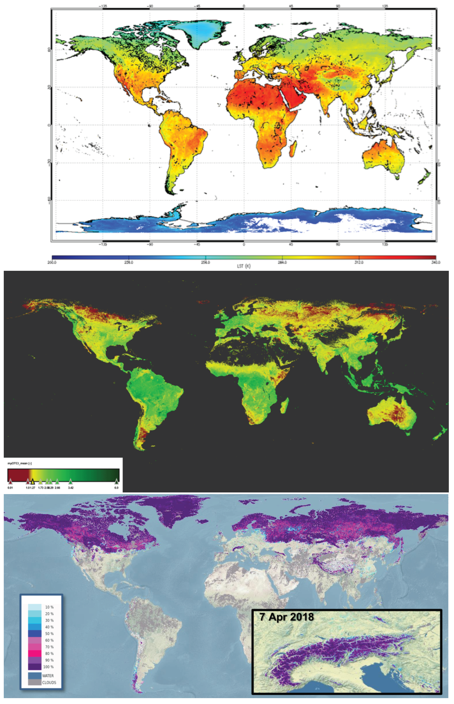
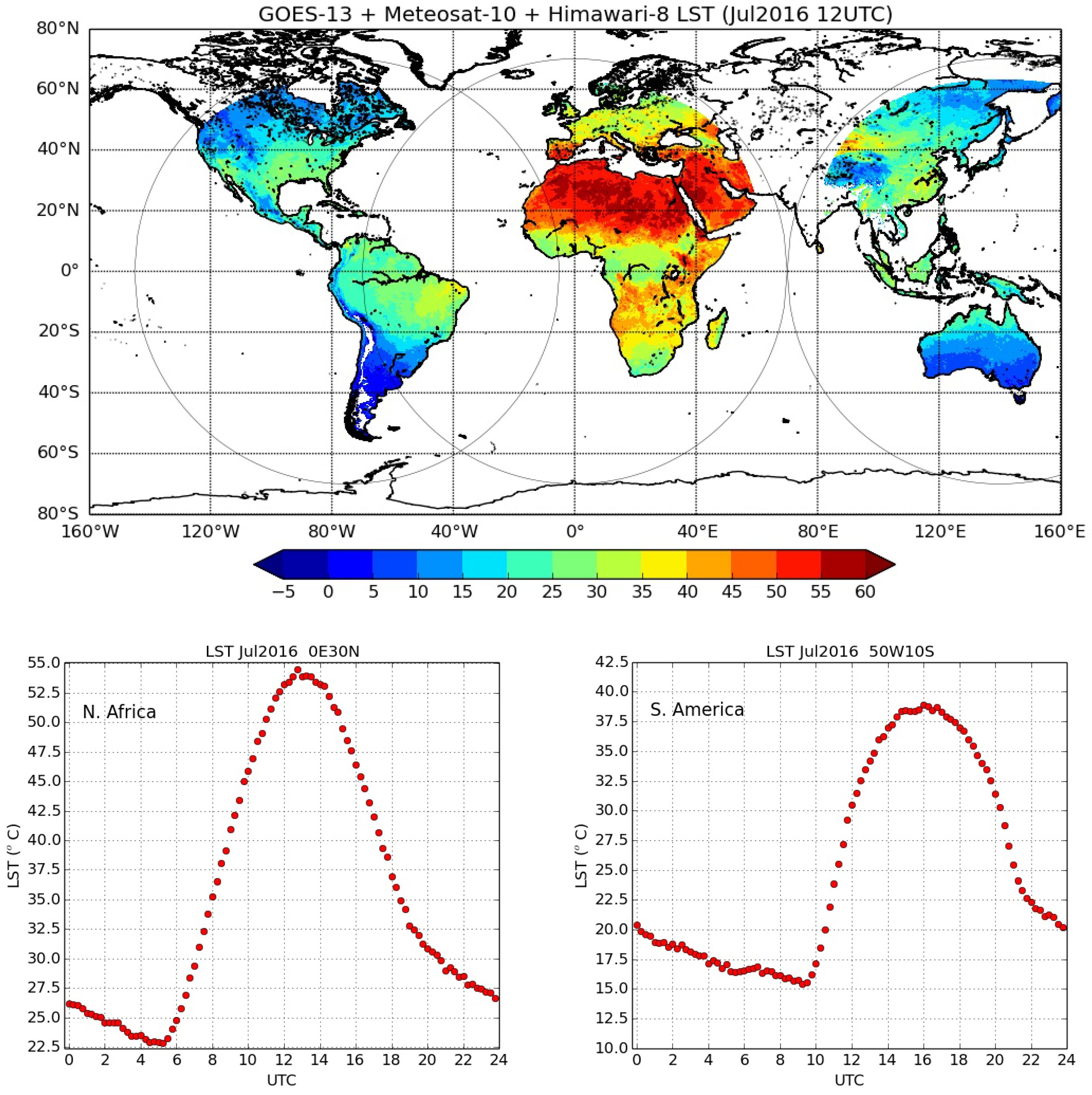
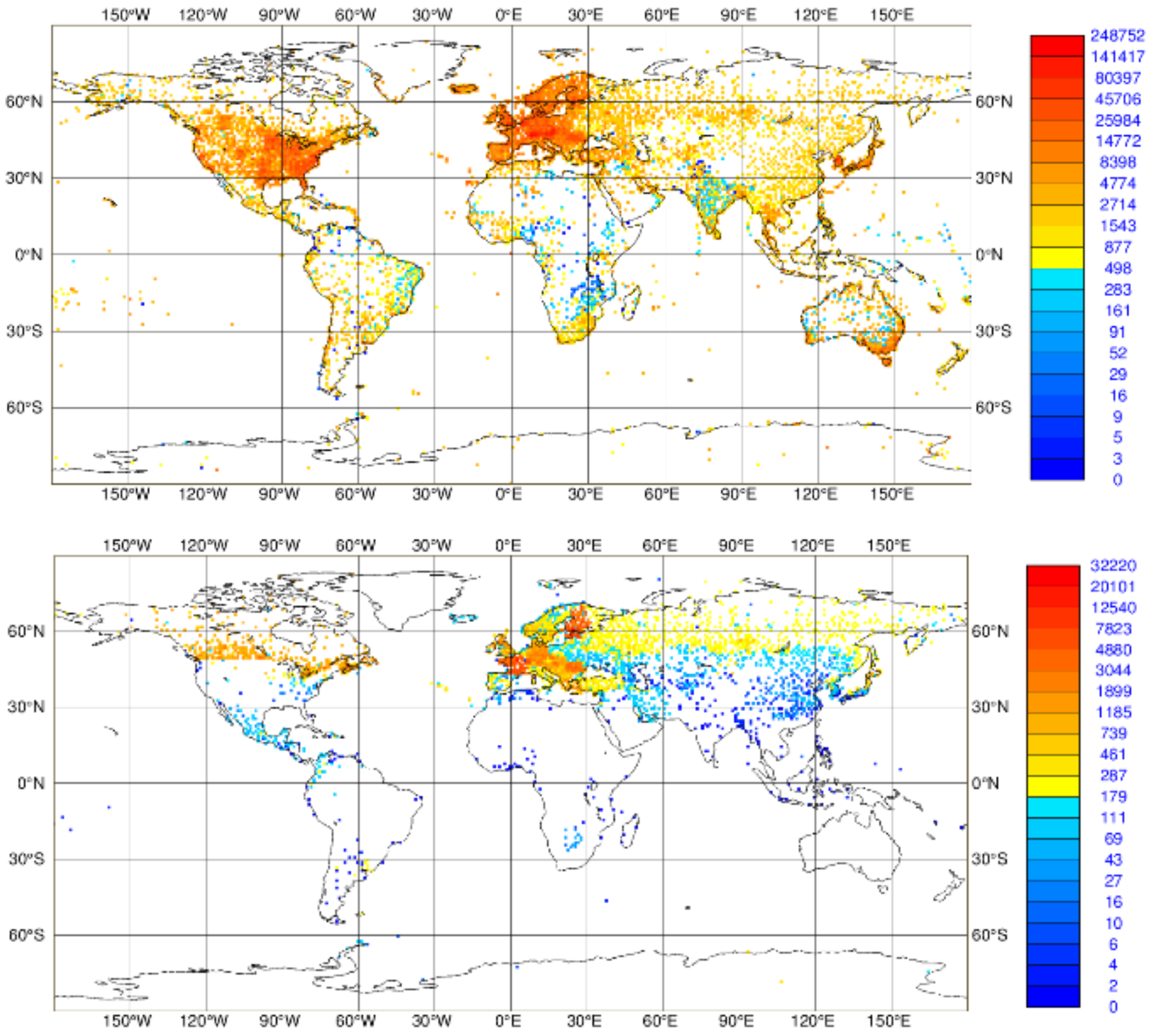
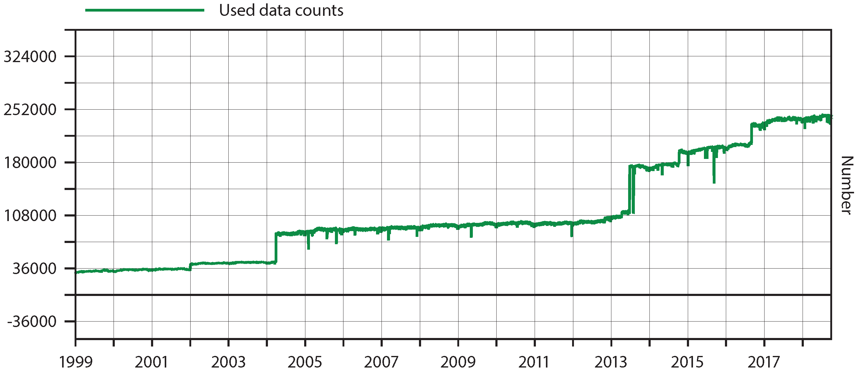
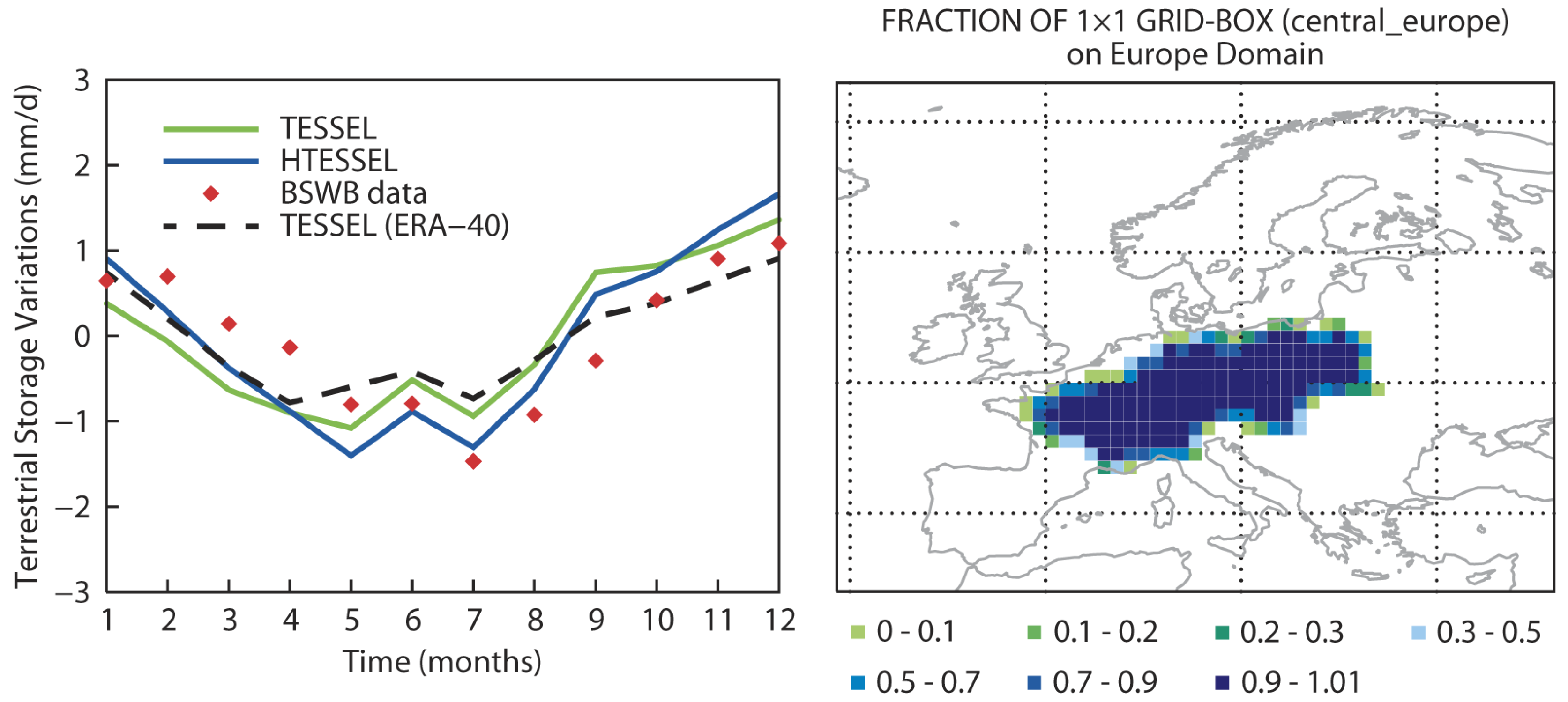
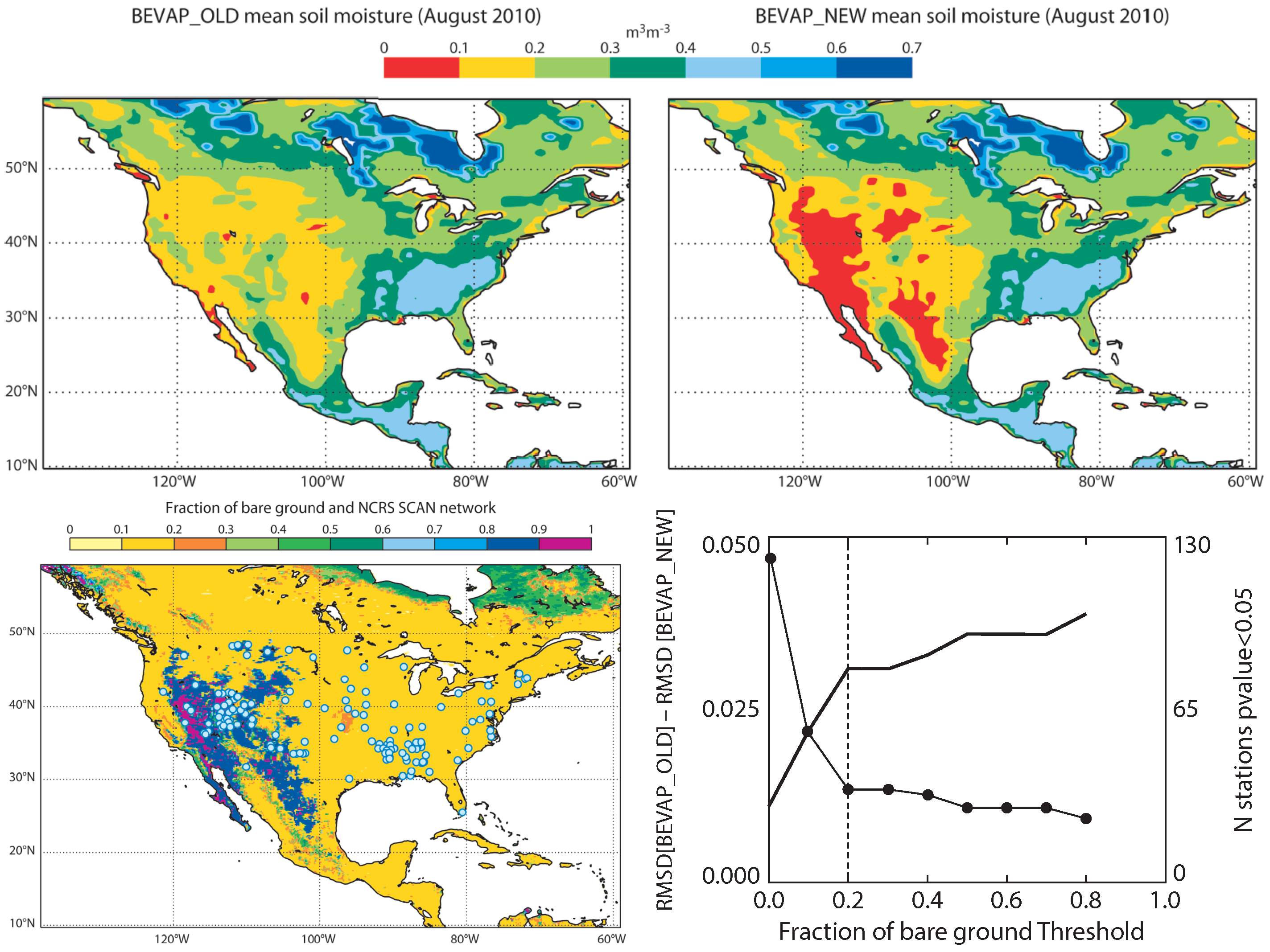
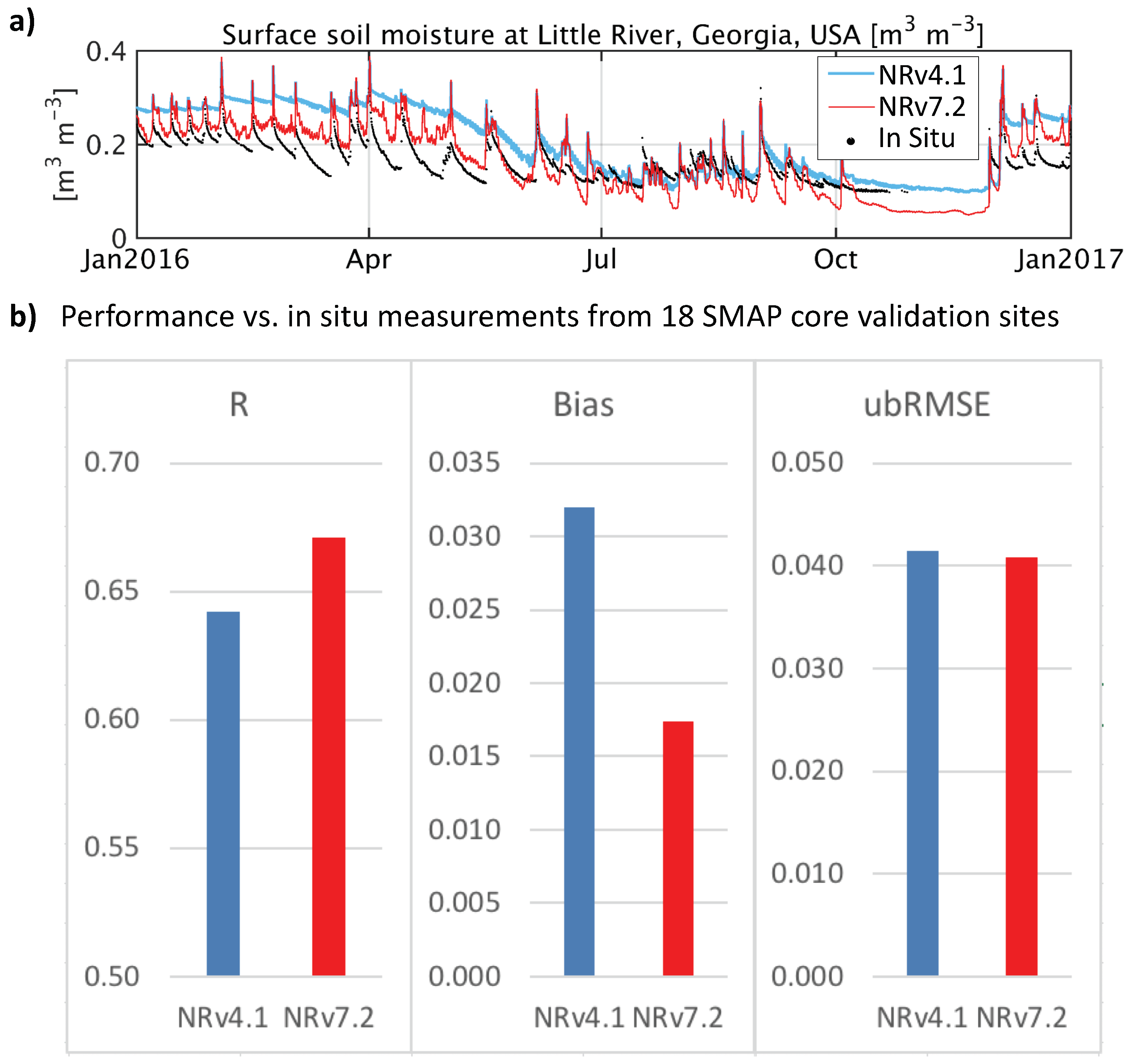
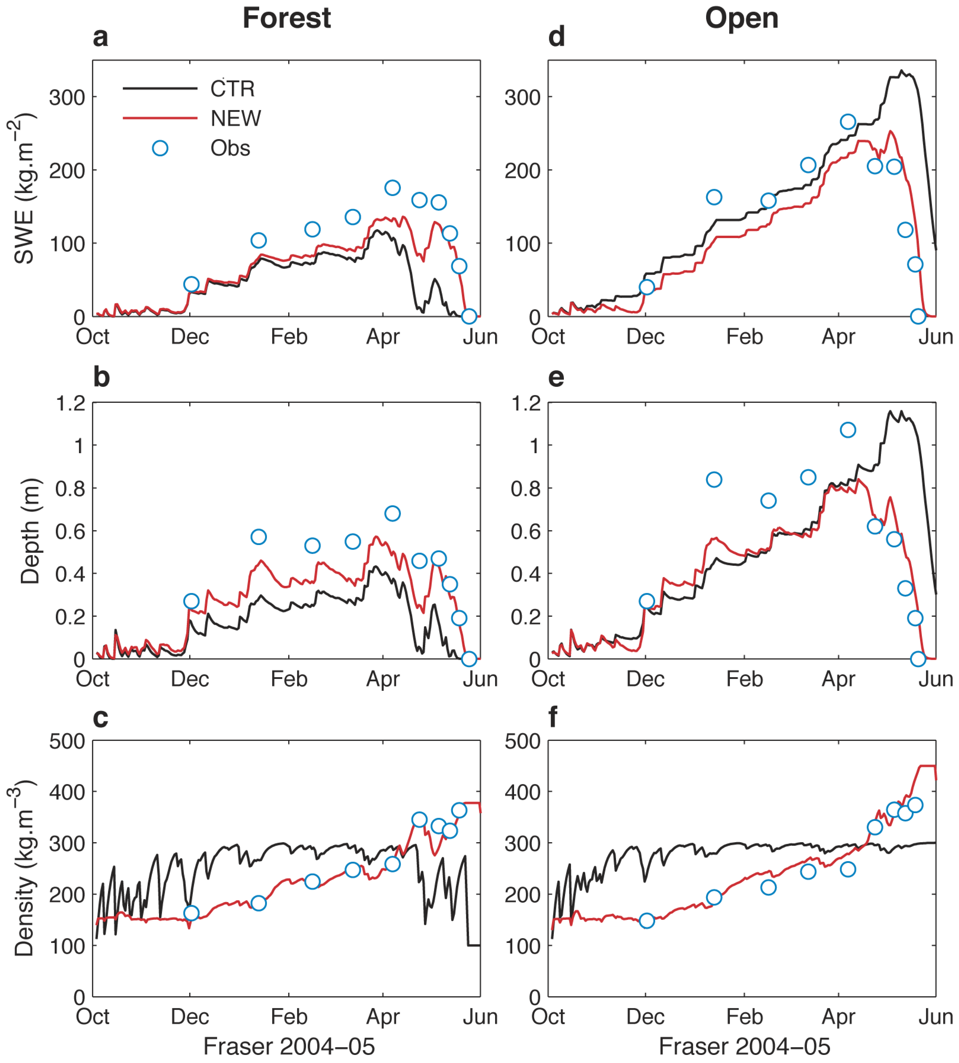
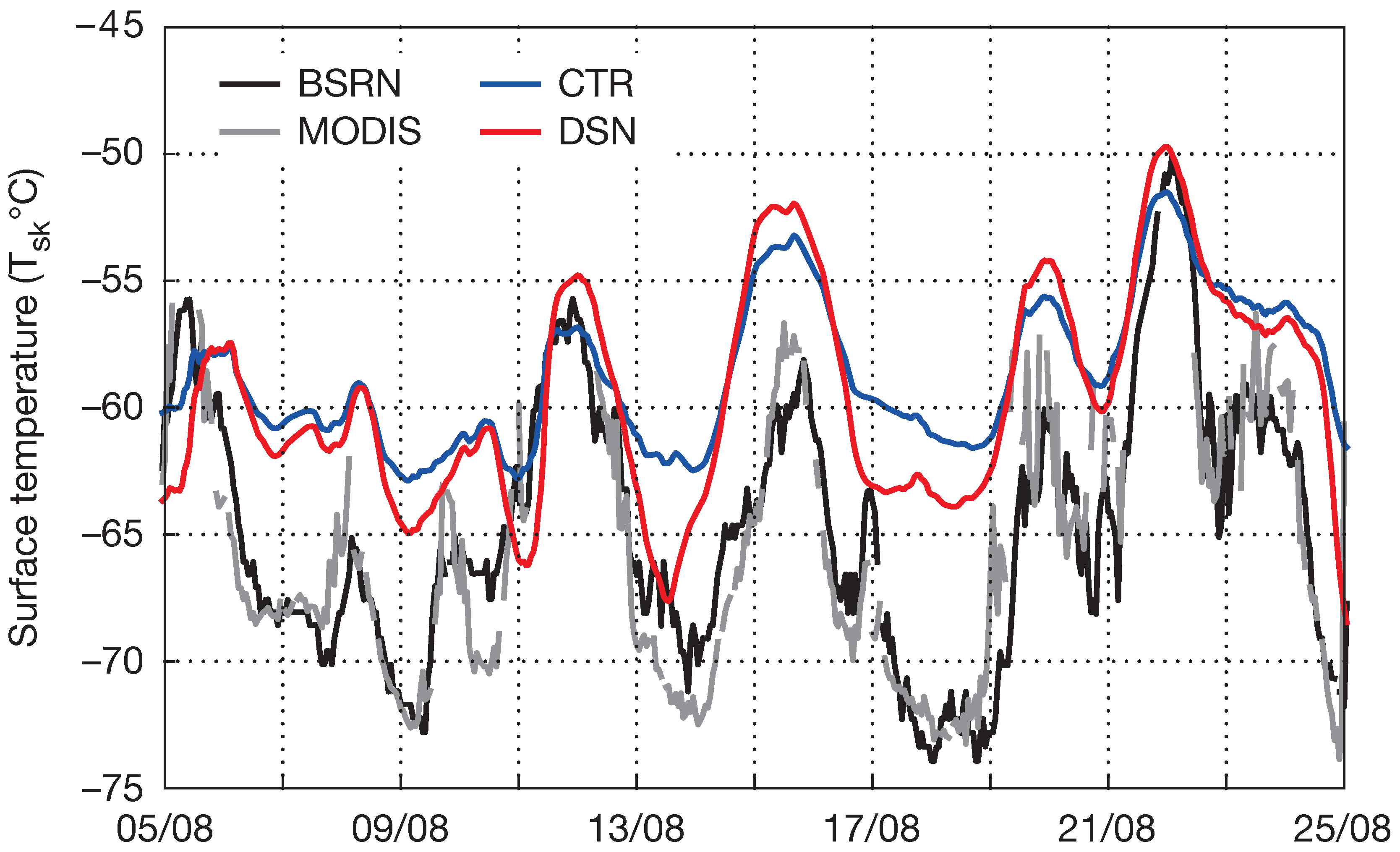
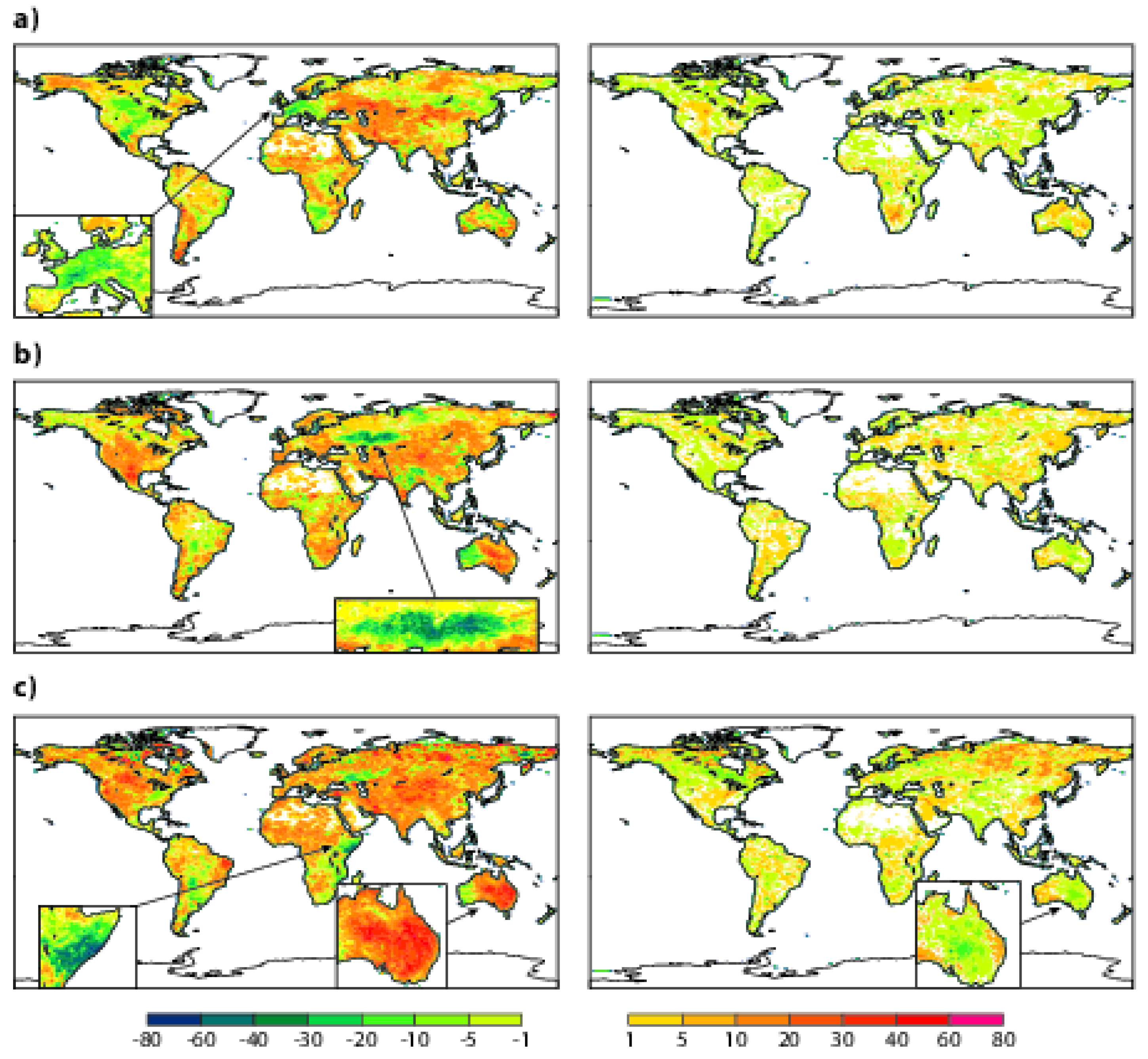
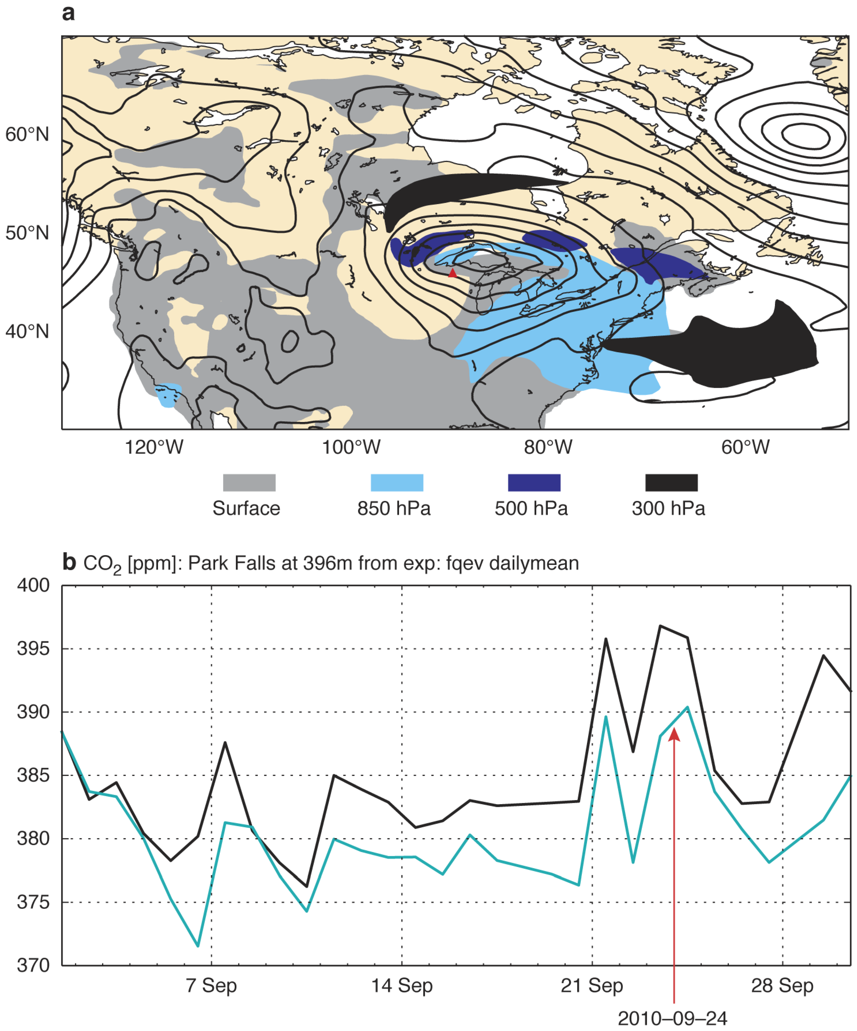
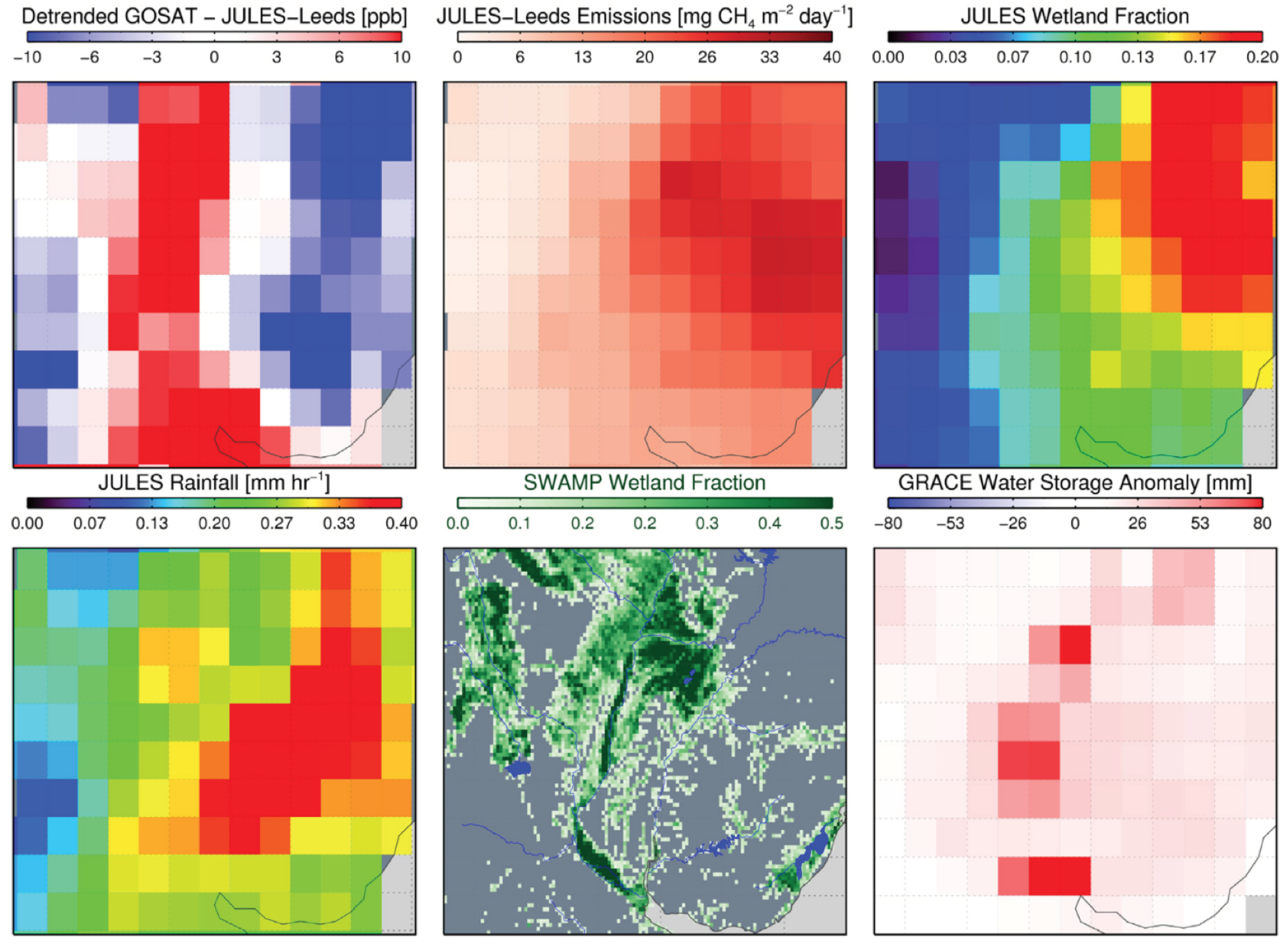
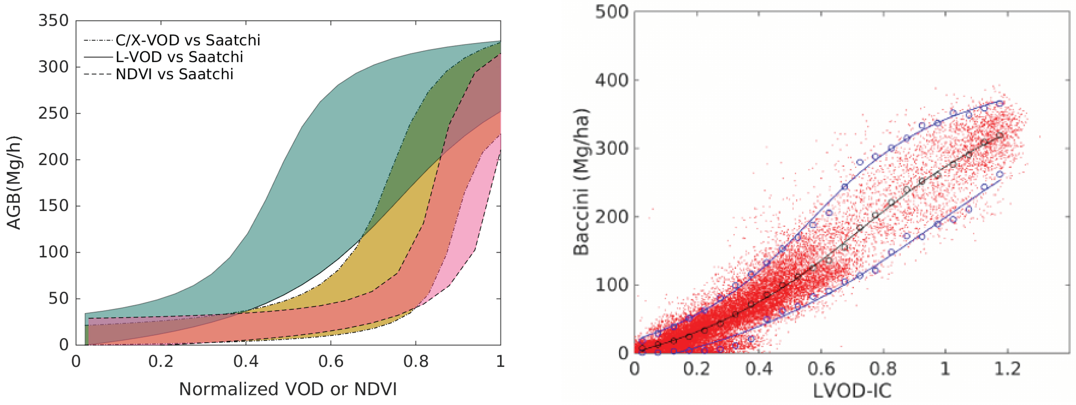
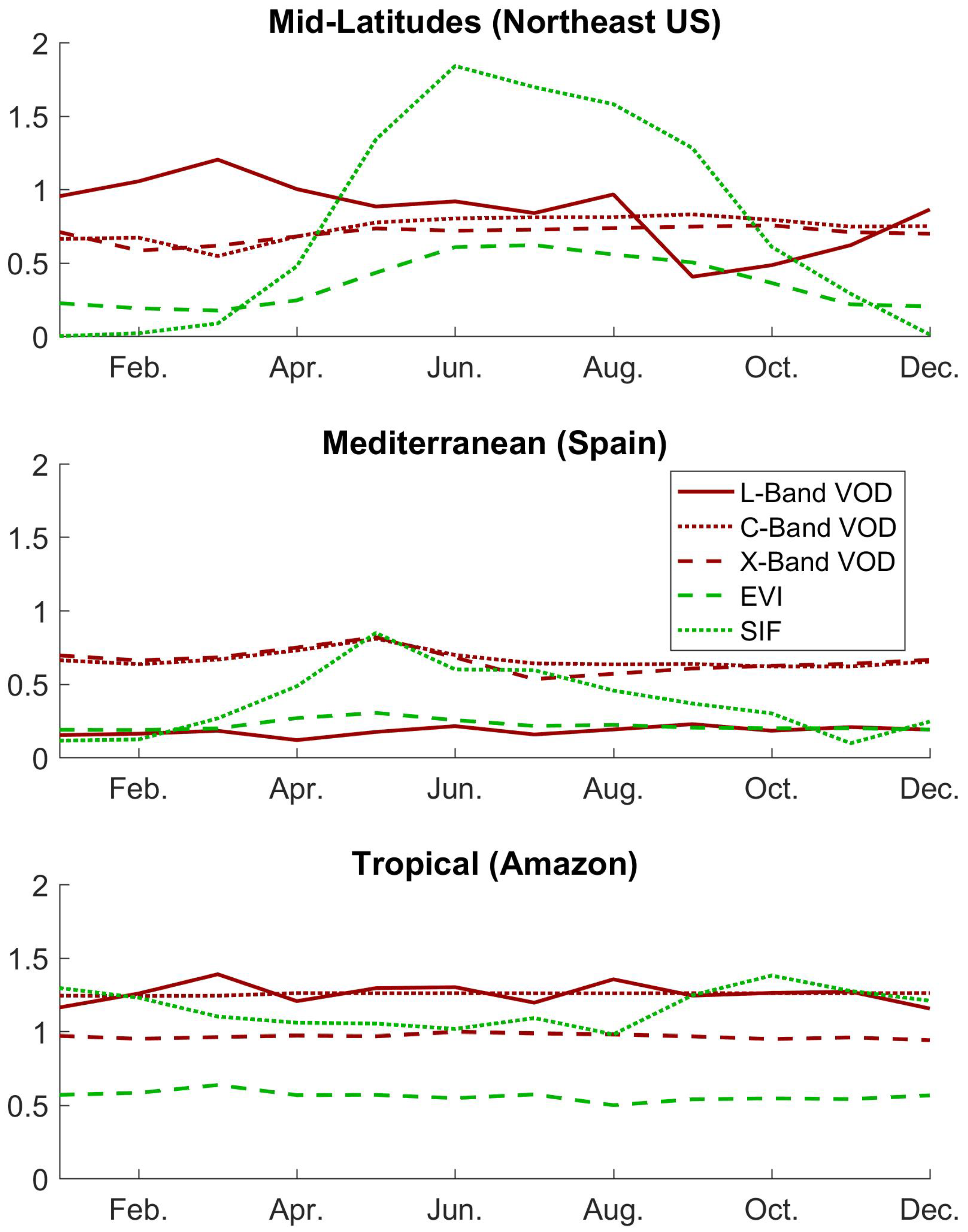
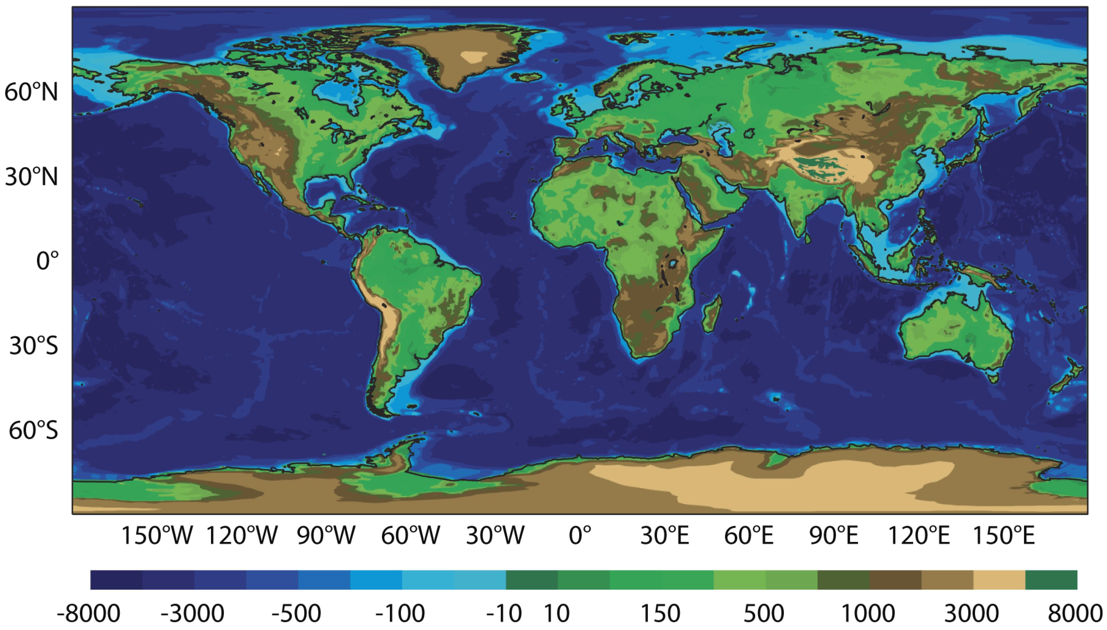
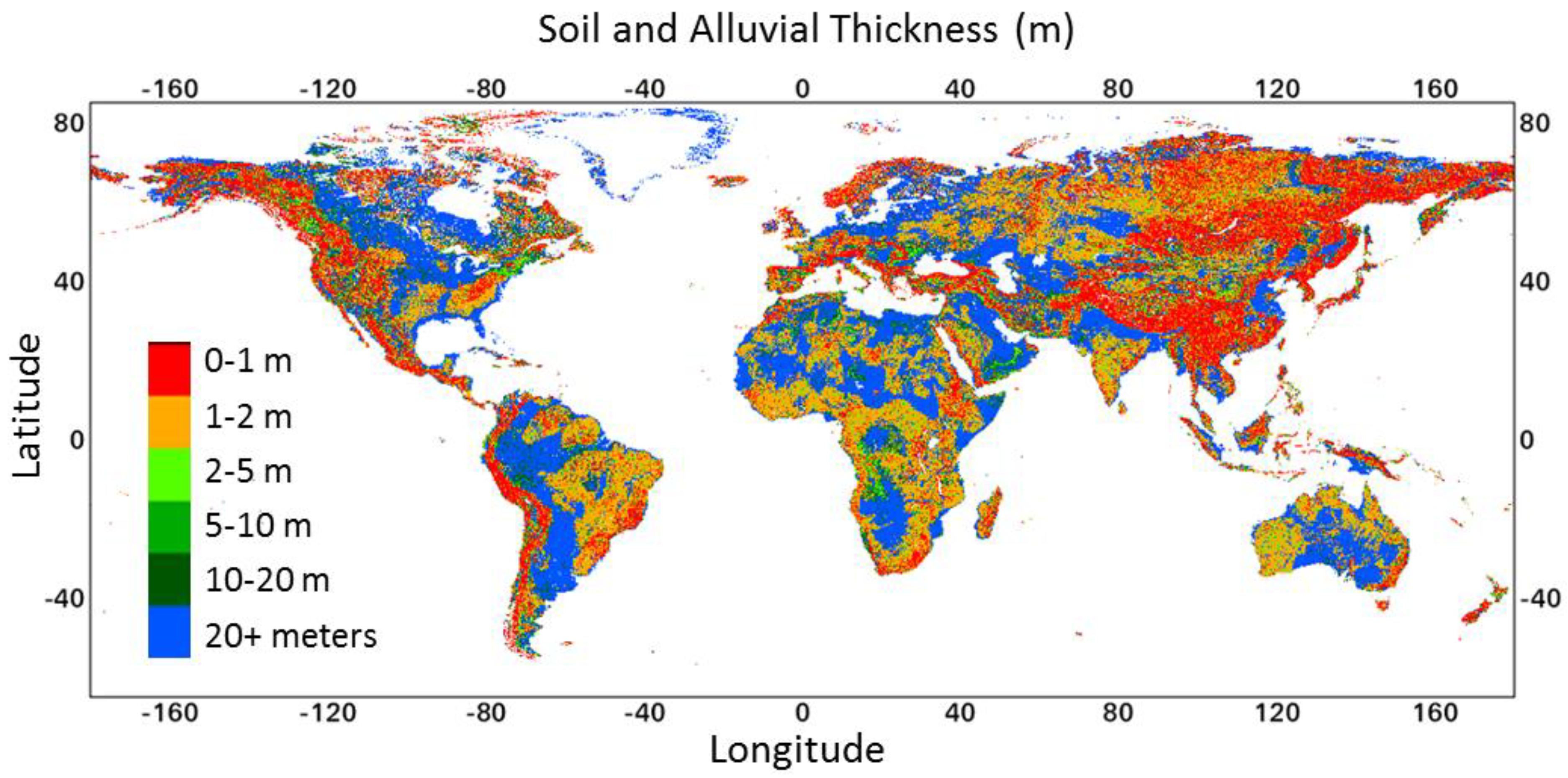
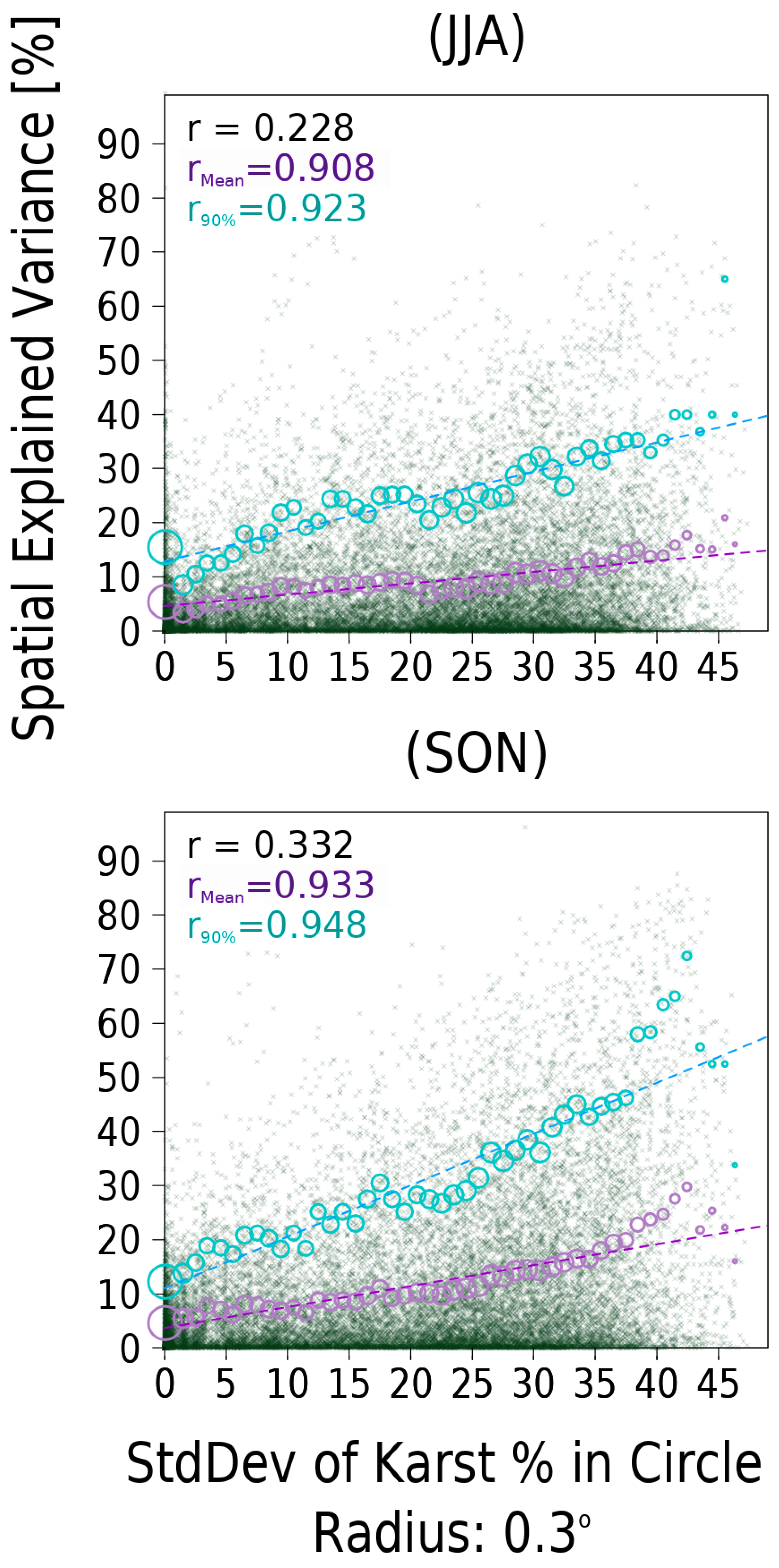
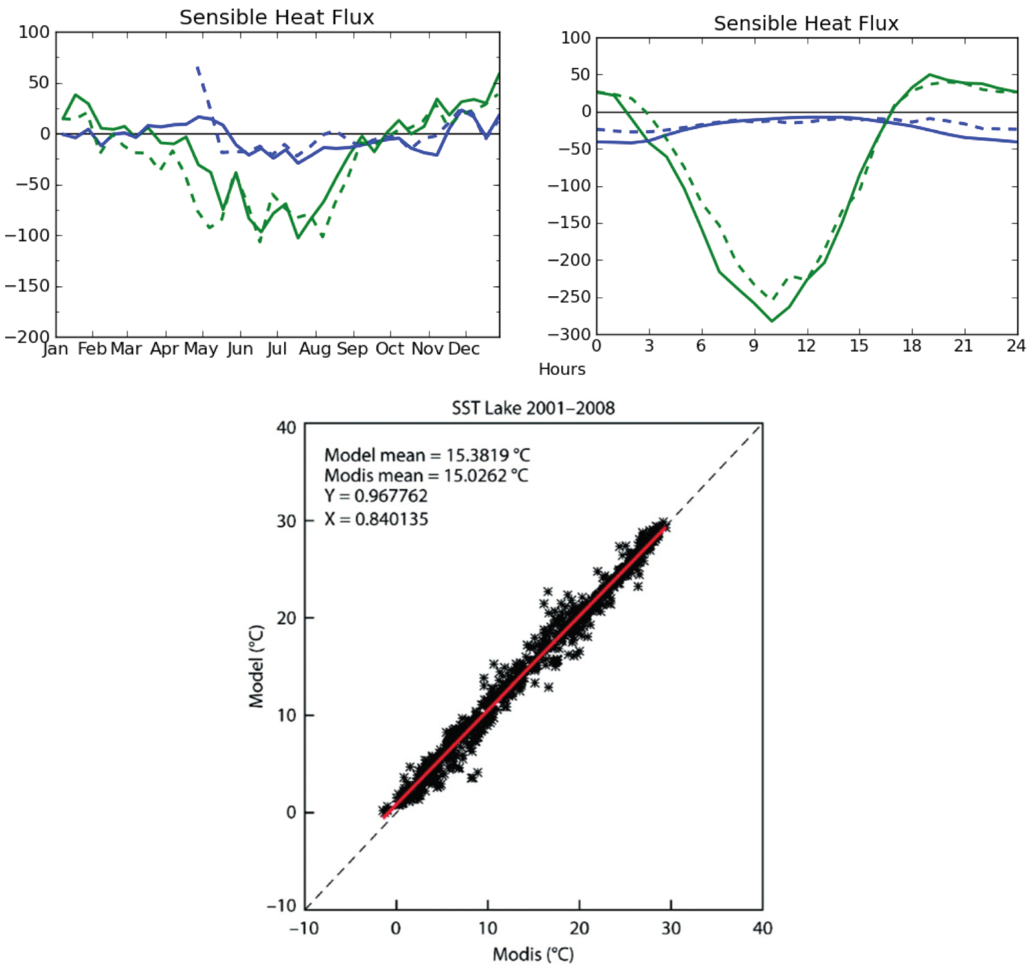
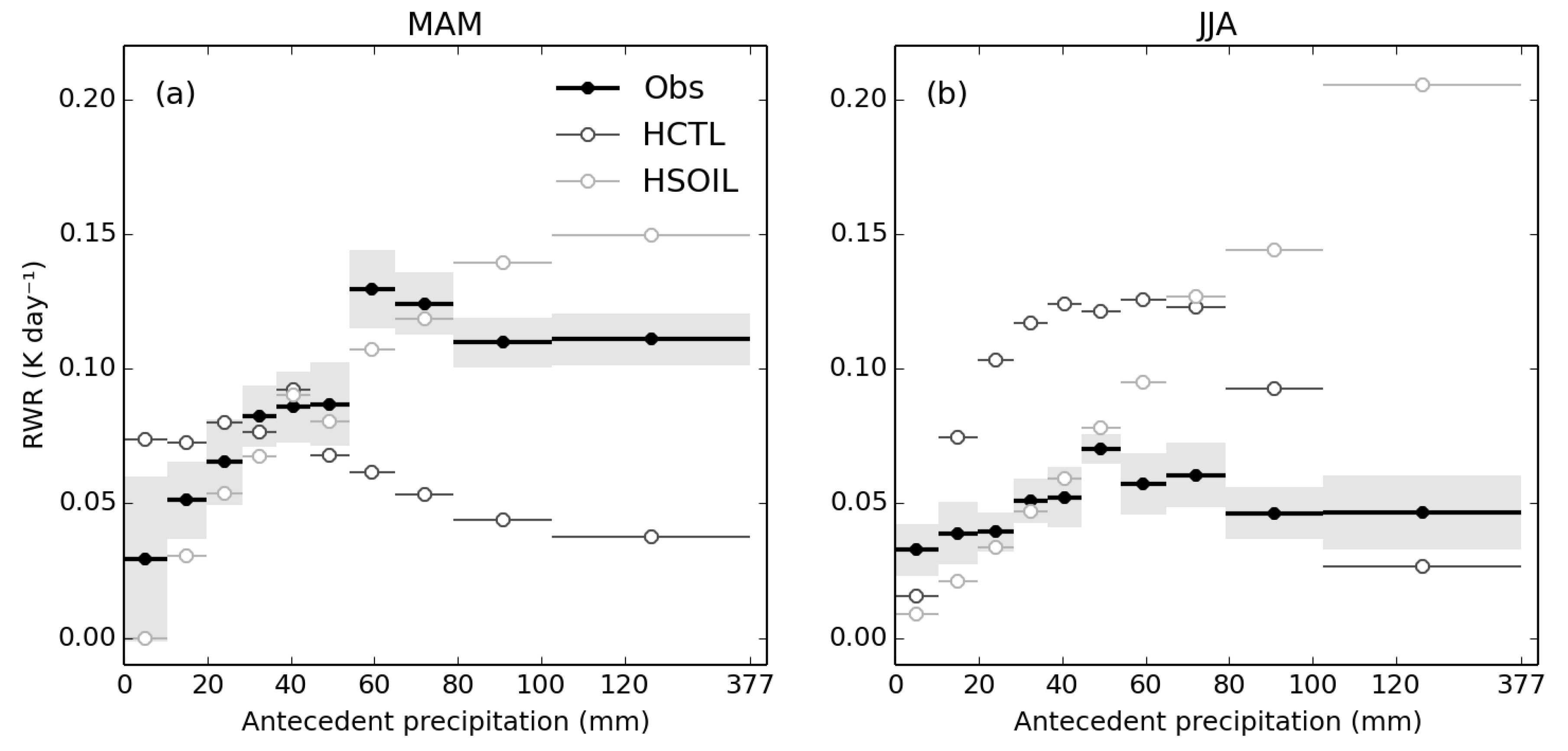
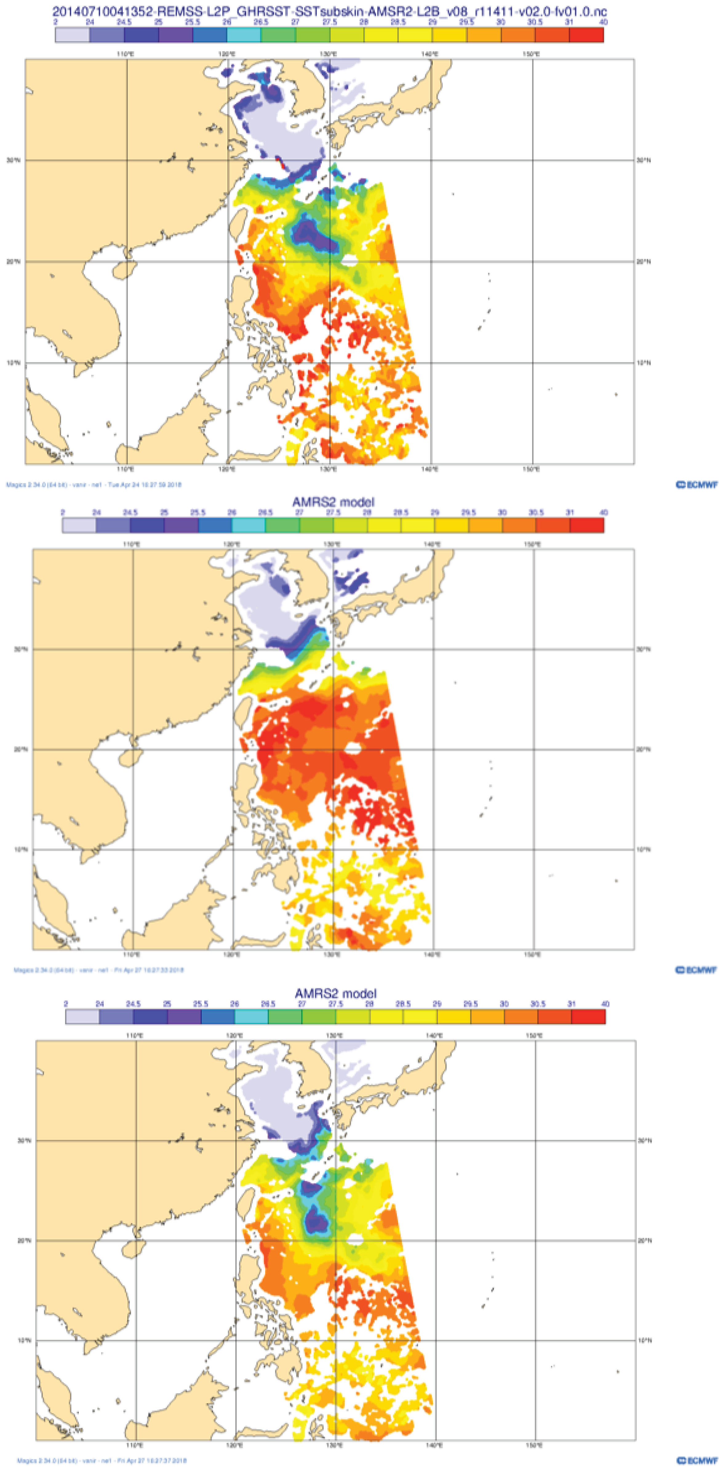
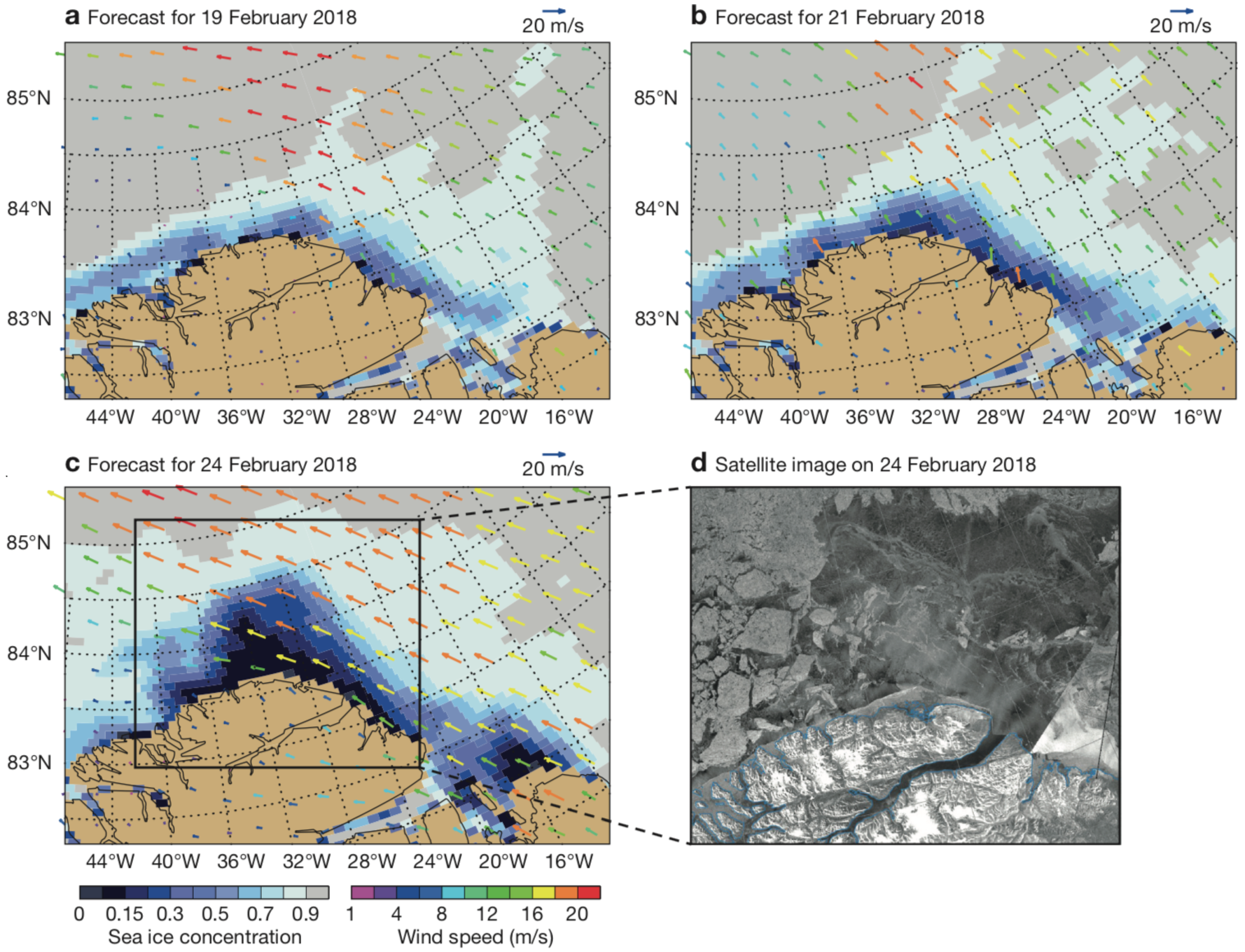
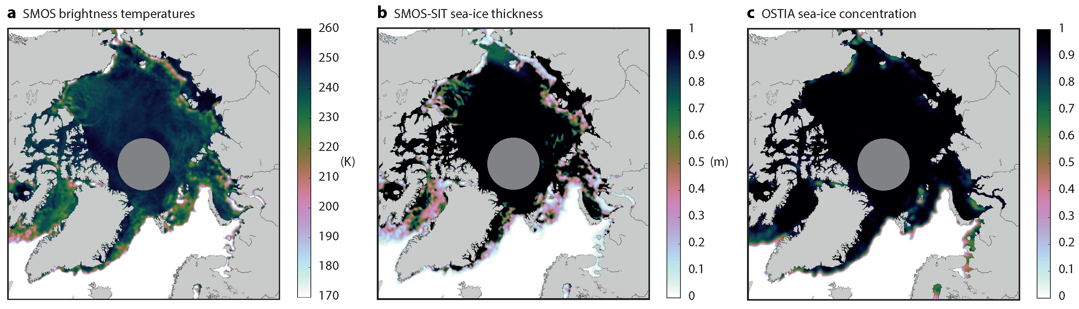
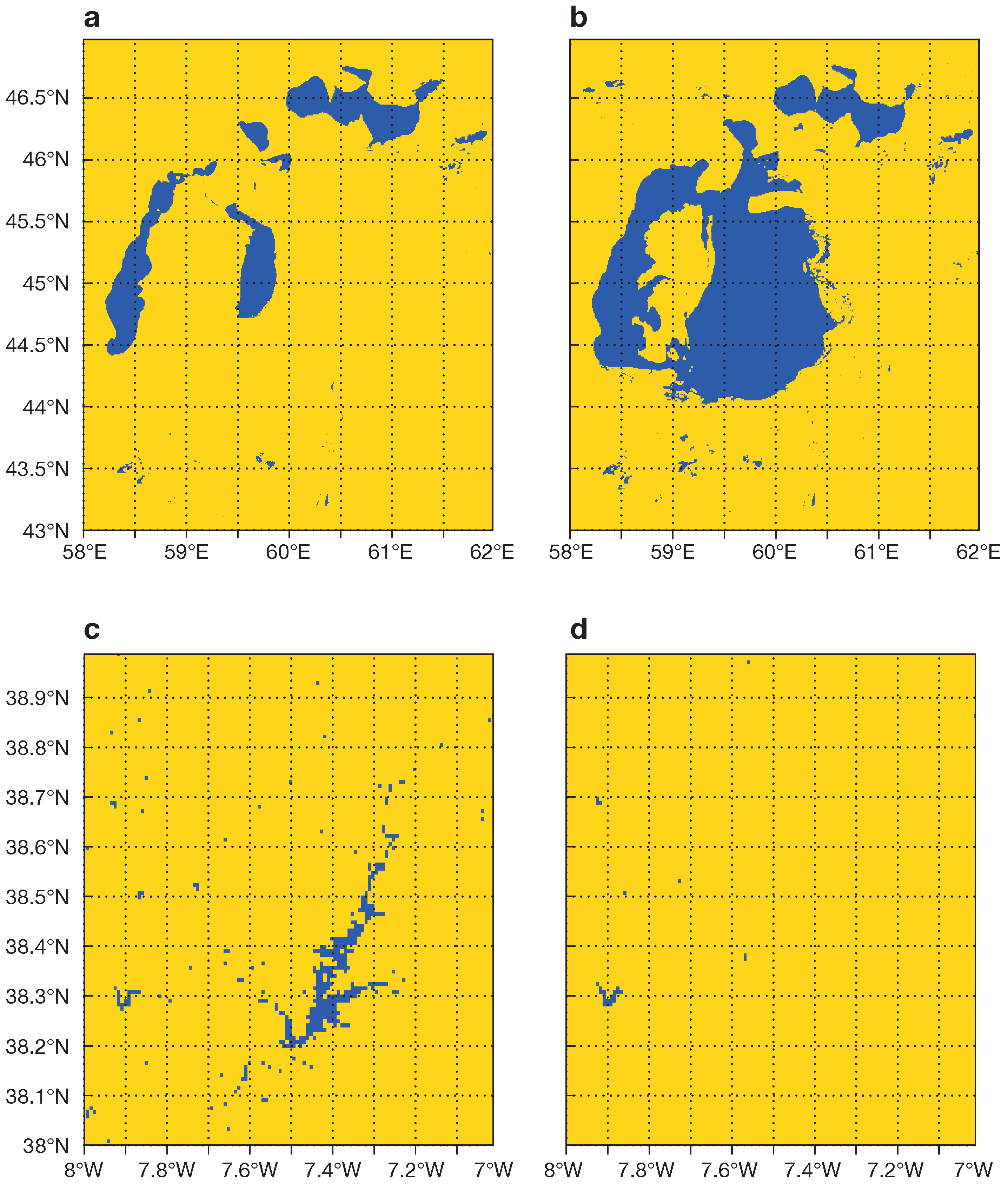
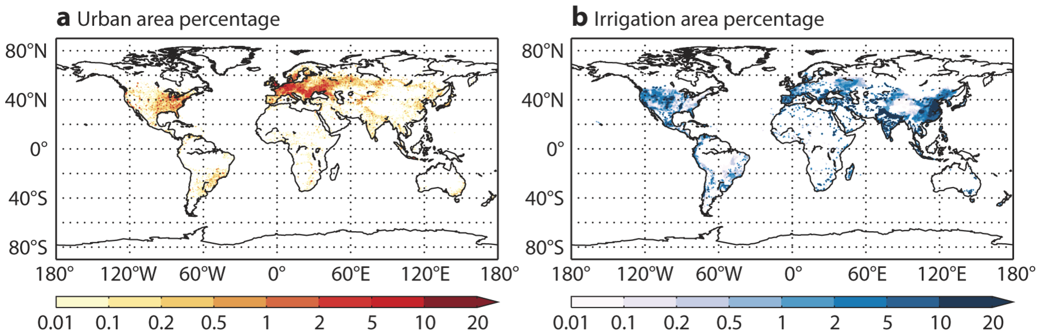
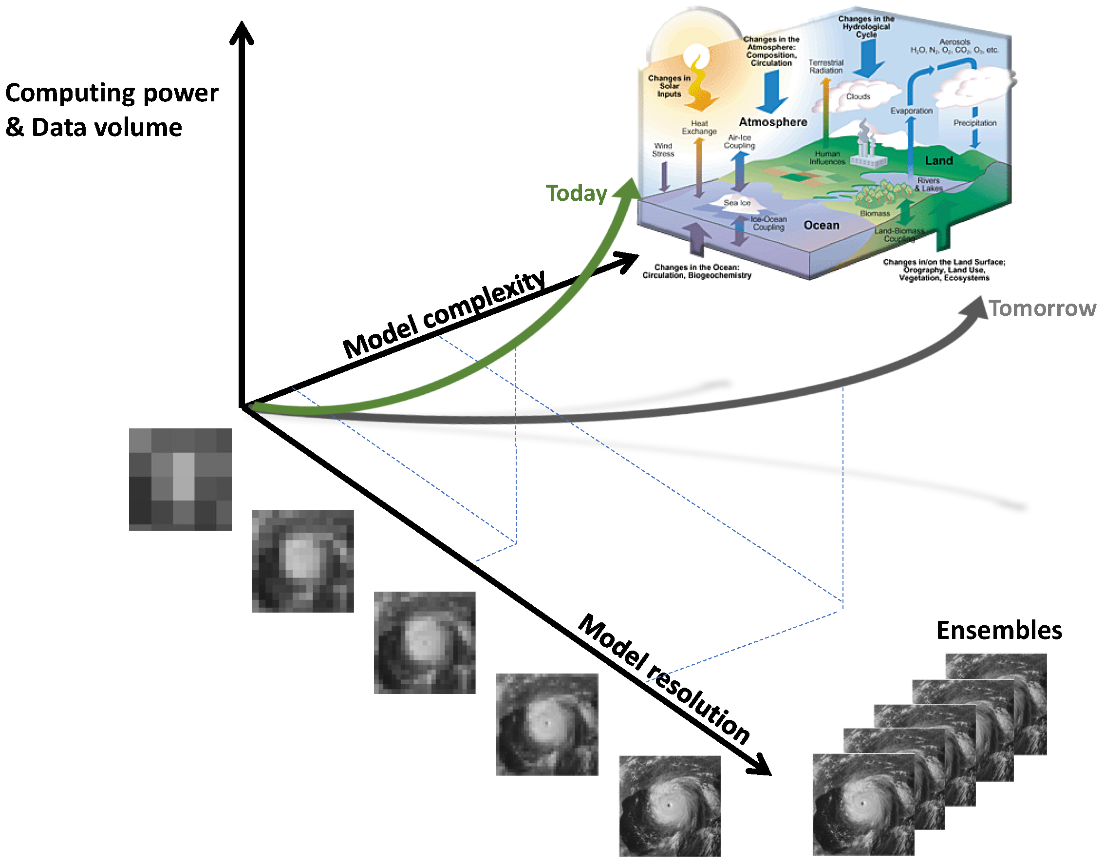
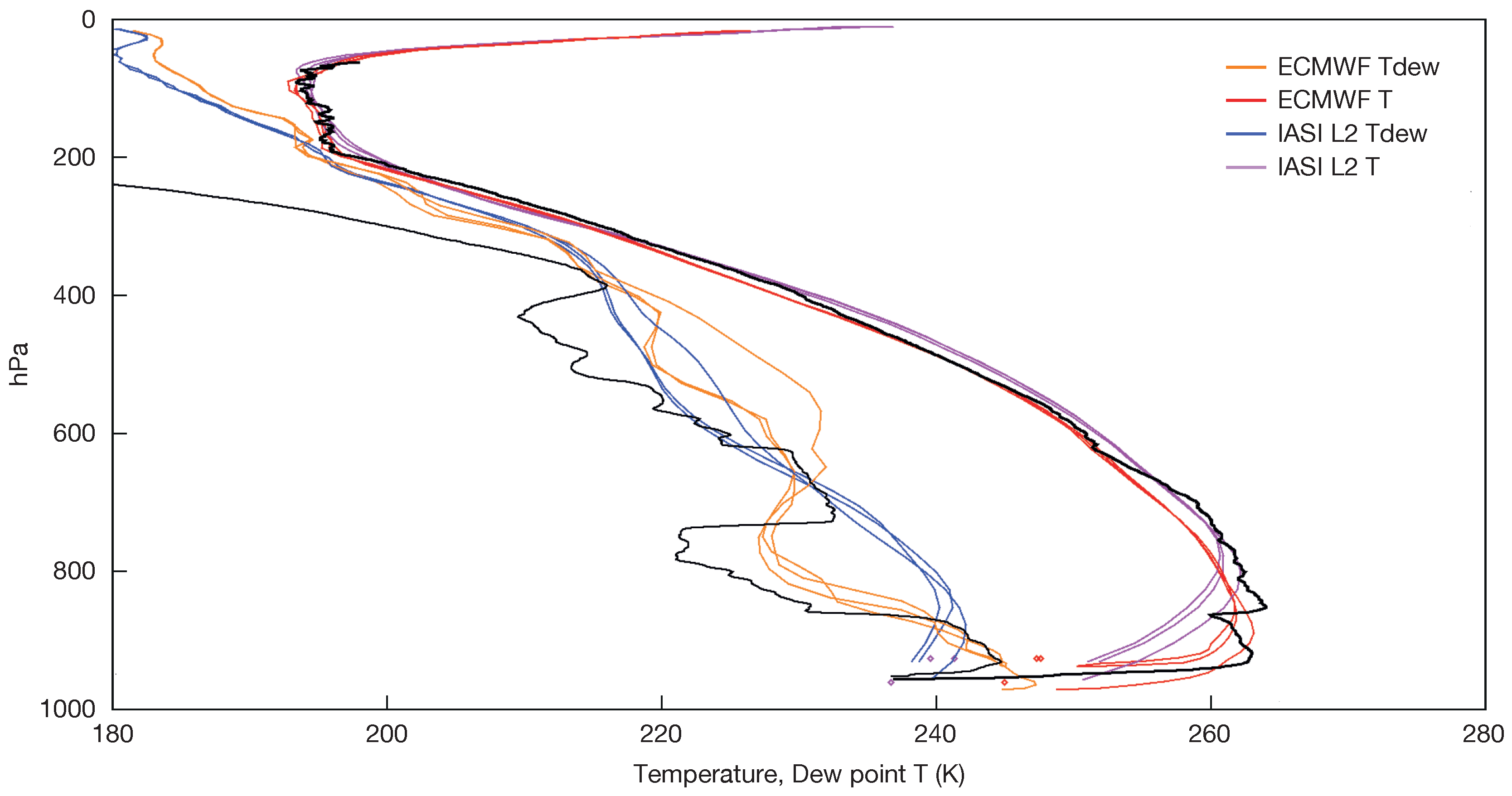
| Sentinel 1 | Launch Date | ESM Relevance |
|---|---|---|
| Sentinel 1A | 3 April 2014 | aggregate |
| Sentinel 1B | 25 April 2016 | aggregate |
| Sentinel 2A | 23 June 2015 | aggregate |
| Sentinel 2B | 7 March 2017 | aggregate |
| Sentinel 3A | 16 February 2016 | direct |
| Sentinel 3B | 25 April 2018 | direct |
| Sentinel 5P | 13 October 2017 | direct |
| Sentinel 6 | 2020 (expected) | direct |
| Geostationary Satellite | Agency | Operating Longitude | Area Coverage |
|---|---|---|---|
| Meteosat First Generation series (up to Meteosat-7) | EUMETSAT | 0°E; 57°E–63°E; 50°W | Africa, Europe, partly South America; Indian Ocean Coverage |
| MSG series (Meteosat-8 to Meteosat-11) | EUMETSAT | 0°E; 9.5°E; 45°E | Africa, Europe, partly South America; Indian Ocean Coverage |
| GOES-East/West | NOAA | 75°W; 135°W | East Satellite: North and South America, Atlantic Ocean; West Satellite: North and South America, Pacific Ocean |
| GOMS-2 | Roshydromet | 76°E | Eurasia, Indian Ocean |
| INSAT-3D | ISRO | 82°E | Asia, Indian Ocean |
| FY-2 | CMA | 86.5°E; 105°E; 112°E | Asia, Indian Ocean, Australia |
| MTSAT-2 | JMA | 145°E | Asia, Indian and Western Pacific Ocean, Australia (inactive since 10 March 2017) |
| Himawari | JMA | 140°E | Asia, Indian and Western Pacific Ocean, Australia |
© 2018 by the authors. Licensee MDPI, Basel, Switzerland. This article is an open access article distributed under the terms and conditions of the Creative Commons Attribution (CC BY) license (http://creativecommons.org/licenses/by/4.0/).
Share and Cite
Balsamo, G.; Agusti-Panareda, A.; Albergel, C.; Arduini, G.; Beljaars, A.; Bidlot, J.; Blyth, E.; Bousserez, N.; Boussetta, S.; Brown, A.; et al. Satellite and In Situ Observations for Advancing Global Earth Surface Modelling: A Review. Remote Sens. 2018, 10, 2038. https://doi.org/10.3390/rs10122038
Balsamo G, Agusti-Panareda A, Albergel C, Arduini G, Beljaars A, Bidlot J, Blyth E, Bousserez N, Boussetta S, Brown A, et al. Satellite and In Situ Observations for Advancing Global Earth Surface Modelling: A Review. Remote Sensing. 2018; 10(12):2038. https://doi.org/10.3390/rs10122038
Chicago/Turabian StyleBalsamo, Gianpaolo, Anna Agusti-Panareda, Clement Albergel, Gabriele Arduini, Anton Beljaars, Jean Bidlot, Eleanor Blyth, Nicolas Bousserez, Souhail Boussetta, Andy Brown, and et al. 2018. "Satellite and In Situ Observations for Advancing Global Earth Surface Modelling: A Review" Remote Sensing 10, no. 12: 2038. https://doi.org/10.3390/rs10122038
APA StyleBalsamo, G., Agusti-Panareda, A., Albergel, C., Arduini, G., Beljaars, A., Bidlot, J., Blyth, E., Bousserez, N., Boussetta, S., Brown, A., Buizza, R., Buontempo, C., Chevallier, F., Choulga, M., Cloke, H., Cronin, M. F., Dahoui, M., De Rosnay, P., Dirmeyer, P. A., ... Zeng, X. (2018). Satellite and In Situ Observations for Advancing Global Earth Surface Modelling: A Review. Remote Sensing, 10(12), 2038. https://doi.org/10.3390/rs10122038