Use of Sun-Induced Chlorophyll Fluorescence Obtained by OCO-2 and GOME-2 for GPP Estimates of the Heihe River Basin, China

Abstract

Sun-induced chlorophyll fluorescence (SIF) provides a new method for monitoring vegetation photosynthesis from space and has been widely used to estimate gross primary productivity (GPP). However, the ability of SIF obtained from the Orbital Carbon Observatory 2 (OCO-2 SIF) and Global Ozone Monitoring Experiment-2 (GOME-2) to estimate GPP in the cold and arid region of Heihe River Basin remains unclear because previous comparisons were insufficient. Here, we choose maize and alpine meadow to evaluate the performance of SIF obtained by OCO-2 and GOME-2 in GPP estimations. The results of this study show that daily SIF₇₅₇ had stronger correlations with daily tower GPP than daily SIF₇₇₁, and the correlation between daily SIF₇₅₇ and daily tower GPP was stronger than the correlation between 16-d averaged SIF₇₄₀ and 16-d averaged tower GPP. The 16-d averaged absorbed photosynthetically active radiation (APAR) and reconstructed sun-induced fluorescence (RSIF) had the strongest linear correlations with 16-d averaged tower GPP. GPP_VPM and GPP_RSIF exhibited the best performance in GPP estimation, closely followed by GPP_SIF₇₅₇, then GPP_SIF₇₇₁ and GPP_ SIF₇₄₀. We also found that the robustness of the correlation coefficients of OCO-2 SIF with GOME-2 SIF was highly dependent on the size of their spatial footprint overlaps, indicating that the spatial differences between OCO-2 and GOME-2 footprints contribute to the differences in GPP estimates between OCO-2 and GOME-2. In addition, the differences of viewing zenith angle (VZA), cloud contamination, scale effects, and environmental scalars (T_scalar × W_scalar) can result in differences between OCO-2 SIF and GOME-2 SIF.

1. Introduction

Plant photosynthesis, termed gross primary productivity (GPP), is the main source of energy for all life on Earth [1], and it drives ecosystem functions and carbon cycling [2]. Accurate estimations of GPP play important roles in the global land carbon budget in the context of global warming [3,4]. As the most effective method of estimating regional-scale GPP, remote sensing has been widely used in carbon cycle studies over the last few decades.

In traditional remote sensing GPP estimation methods, GPP is calculated using light use efficiency (LUE) models based on vegetation indices (such as the normalized difference vegetation index [NDVI] and enhanced vegetation index [EVI]) and auxiliary meteorological data (such as temperature and solar radiation) as inputs. A variety of LUE models have been developed with different combinations of vegetation indices and environmental stress expressions, such as the vegetation photosynthesis model (VPM) [5], the moderate-resolution imaging spectroradiometer photosynthesis (MODIS-PSN) algorithm [6], the Carnegie Ames Stanford Approach (CASA) model [7], and the eddy covariance (EC)-based LUE (EC-LUE) model [8]. Vegetation indices based on reflectance can track the greenness well, however, they are less sensitive to actual variations in photosynthesis [9,10,11]. Vegetation indices such as NDVI cannot reflect diurnal physiological changes caused by heat and water stress [12]. LUE models such as the MODIS GPP algorithm require many variables, including auxiliary meteorological data, the use of these data can result in uncertainty to the estimations of GPP [13]. With the rapid development of remote sensing techniques, machine learning methods have become a very useful tool to process GPP-related data. Global flux products were simulated by using the machine learning methods to scale EC data up remote sensing data [14]. The basal areas of spruce and fir were mapped by using machine learning techniques in conjunction with remote sensing and measurement data in Central Siberia [15].

Sun-induced chlorophyll fluorescence (SIF) data have been reported to be a promising new tool to accurately monitor GPP [16,17,18]. Light energy absorbed by the leaf chlorophyll molecules has three different pathways: Photochemistry, nonphotochemical quenching (NPQ, i.e., heat dissipation), and a small amount of energy emitted as SIF at long wavelengths [19,20]. Complementing reflectance-based vegetation indices, space-borne SIF observations are excellent indicators of the vegetation photosynthesis process and these observations provide a new method of monitoring photosynthesis from space [19,21,22,23,24,25,26,27,28,29,30,31].

Recently, several studies evaluated SIF using GPP observed by the EC technique. SIF has been used to capture the seasonal variations in crops in Nebraska, USA [24]. Satellite SIF data have been shown to be correlated with the canopy photosynthesis at diurnal and seasonal scales in a mixed temperate forest in central Massachusetts, USA; thus, SIF can be used as a proxy for GPP [22]. SIF has been reported to accurately capture seasonal and interannual GPP dynamics across dryland ecosystems in Southwestern North America [32]. Global Ozone Monitoring Experiment-2 (GOME-2) SIF data have been used to monitor time-resolved photosynthesis in the US corn belt and European grassland, and reports have indicated that SIF-based crop GPP estimates are 50–75% higher than the results from state-of-the-art carbon cycle models [33]. Moreover, researchers have performed initial evaluations of the use of Orbital Carbon Observatory 2 (OCO-2 SIF) SIF to estimate GPP for crops in the Minneapolis-Saint Paul metropolitan area [34], grass at an OzFlux grassland site [35], and temperate forests in Northern Wisconsin, USA [31]. SIF-based GPP models have been rapidly developed [24,31,36], including a simple regression GPP model [33] and a nonlinear GPP-SIF model [31], and reports have indicated that temporal correlations with GPP can be improved by spatially downscaling SIF [37]. More recently, reconstructed sun-induced fluorescence (RSIF) product was created, which utilizes high resolution MODIS data to predict GOME-2 SIF data, and the results indicated that RSIF had much higher seasonal and interannual correlation than the original SIF, especially in dry and cold regions [38]. Most of the above studies were conducted in the USA and Western Europe, and few studies have compared the GPP estimates from SIF retrievals from GOME-2 and OCO-2 in China. If the difference between the results of these methods and whether SIF exhibits the same performance in GPP estimates in the cold and arid region of China remains unclear. Therefore, it is interesting to evaluate the performance of SIF in the cold and arid region of China. Specifically, the differences in SIF retrievals from GOME-2 and OCO-2 must be evaluated to determine whether they perform consistently in GPP estimations and identify the extent to which different spatial resolutions contribute to the differences.

In this study, the objectives were to (1) examine the correlations between tower GPP and GOME-2 SIF data at one retrieval band (740 nm), and OCO-2 SIF data at two retrieval bands (757 nm and 771 nm); (2) assess the performance of a SIF-based GPP model and a traditional LUE model (VPM); and (3) find possible reasons for the differences between OCO-2 SIF and GOME-2 SIF.

2. Materials and Methods

2.1. Study Sites

The Heihe River Basin (97°24′–102°10′ E and 37°41′–42°42′ N), located in Northwest China, is the second largest inland river basin in China. The Daman superstation and A’rou superstation in the Heihe River Basin were chosen for this study because they collect high-quality EC observations and are located in typical ecosystems in the upper and middle streams of the Heihe River Basin (Figure 1). The Daman superstation (100°22′ E, 38°51′ N, 1556 m) was established during the Heihe Watershed Allied Telemetry Experimental Research (HiWATER) experiment in May 2012 in an area of irrigated farmland with maize as the dominant crop [39]. The A’rou superstation (100°27′ E, 38°02′ N, 3033 m) was established during the HiWATER experiment in 2013 in an area of alpine meadow in the upper stream region [39]. EC and meteorological data were collected from two sites and were provided by the Cold and Arid Regions Science Data Center (http://westdc.westgis.ac.cn/). Data on meteorological variables and measured carbon fluxes from 2013 to 2017 at the Daman and A’rou superstations were used in this study.

2.2. Carbon Flux and Meteorological Data Process

Meteorological data were sampled every minute at the Daman and A’rou superstations and then converted to 30 min average values and daily values. The meteorological data were quality controlled by filtering values beyond the physical range or instrument range. The raw 10-Hz EC data were processed to half-hourly flux data via spike detection, lag correction of H₂O/CO₂ relative to the vertical wind component, sonic virtual temperature conversion, coordinate rotation, the Webb-Pearman-Leuning (WPL) correction and frequency response correction [40]. Half-hourly carbon flux data were further partitioned into GPP and ecosystem respiration. The carbon flux value was excluded if the instrument range was excessive, rainfall occurred or instrument malfunctions occurred. At night, carbon flux data were filtered if the friction velocity (u*) was lower than a threshold value (0.15 m/s for Daman and 0.1 m/s for Arou). The gaps in the carbon flux data were filled using the light response function (Michaelis–Menten equation) and respiration function (Van’t Hoff equation) [41]. The ecosystem respiration function (Van’t Hoff equation) was fitted with nighttime net ecosystem exchange (NEE) and air temperature data. Then, the fitted function was applied to the daytime data to estimate ecosystem respiration. The GPP was calculated as the difference between the estimated ecosystem respiration and NEE. The partitioned GPP data were used as ground truth to evaluate the SIF and vegetation indices during the GPP estimation.

2.3. SIF Data

OCO-2 belongs to a sun-synchronous orbit satellite that was launched on 21 September 2014 and has an overpass time at ~1:30 pm. The OCO-2 spectrometer measures spectra in the O₂-A band with far-red SIF retrieved at 757 nm and 771 nm based on the filling in Fraunhofer lines [25,42,43]. OCO-2 data were produced by the OCO-2 project at the Jet Propulsion Laboratory, California Institute of Technology, USA. The sun-sensor acquires data in the nadir, glint, and target modes, with a revisit period of approximate 16 days, and its ground-pixel size is 1.3 × 2.25 km², which directly facilitates local studies. The latest version of the B8100r OCO-2 dataset was used in this study. A conversion factor was provided in the dataset, which was used to convert the instantaneous SIF to a daily average SIF [36]. The OCO-2 SIF retrievals at 757 nm and SIF 771 nm are denoted SIF₇₅₇ and SIF₇₇₁ in this study, respectively. OCO-2 SIF retrievals are noisy as single observations, even though OCO-2 has a small footprint. The OCO-2 SIF retrievals for cloudy days were removed according to the solar radiation measured by the flux tower in this study [44,45].

GOME-2 on MetOp-A platform belongs to a sun-synchronous orbit satellite which was first launched on 19 October 2006 with an overpass time at ~9:30 am. GOME-2 measures spectra for top-of-atmosphere radiance between 240 and 790 nm with a spectral resolution between 0.2 and 0.5 nm, and it has a signal-to-noise ratio of ~1000 and a relatively large footprint (approximately 40 km × 80 km at nadir for MetOp-A before 15 July 2013 and 40 km × 40 km since 15 July 2013) [46]. SIF was retrieved near the wavelength of 740 nm by using a principal component analysis algorithm [47]. The GOME-2 SIF retrievals were quality filtered and controlled (e.g., heavy cloud contamination and data with relatively low signal-to-noise ratios were removed) and binned in 0.5° latitude-longitude grid cells [45,48]. Version 27 (V27) level 2 retrievals are the results of new postprocessing based on Version 26 (V26), and these retrievals provide additional fields (daily-averaged SIF and quality flag, i.e., users can apply quality flags to filter out bad data) and have adjusted bias corrections and calibrations. Only good quality data (quality flag = 2, details are given in Section 2 in the supplementary material) were used in this study. As a new proxy for GPP, RSIF was developed using a machine learning approach based on the inputs-MODIS reflectance to predict GOME-2 SIF data, and detailed parameters on RSIF can be found in a previous study [38].

To remain spatially consistent with GOME-2 SIF retrievals, a 0.5° grid cell based on the coordinates of the flux towers was used to extract the OCO-2 SIF data for the period from September 2014 to December 2017 and to match the GOME-2 SIF at the Daman and A’rou sites. The OCO-2 SIF data were calculated using the averaged values of the available pixels around the towers over a square of 0.5° by 0.5°. GOME-2 SIF values were extracted within a 0.5° grid cell based on the coordinates of the flux towers. The daily-averaged GOME-2 SIF data were noisy as single measurements; thus, they were averaged over a 16-d period to investigate the GPP-SIF relationship. Due to the different platforms, wavelengths and overpass times between OCO-2 and GOME-2, we fitted the GPP-SIF relationship separately. The daily OCO-2 SIF and a 16-d averaged GOME-2 SIF data were used to ensure a reasonable comparison between OCO-2 and GOME-2.

2.4. MODIS Data

The MODIS data used in this study were the MOD09GA (Terra, collection 6) Terra daily surface reflectance (SREF) L2 Global product for the period from 2014–2017, which came from the Land Processes Distributed Active Archive Center (LP DAAC) with a spatial resolution of 500 m. Reflectances for the red (620–670 nm), near-infrared (841–875 nm), blue (459–479 nm), and shortwave infrared bands (1628–1652 nm) were used to calculate the EVI and the land surface water index (LSWI) for 2014–2017. To match the SIF spatial resolution (0.5° latitude and longitude resolution), we calculated vegetation indices (EVI and LSWI) for pixels within a square of 0.5° by 0.5° around the two flux sites, and good-quality data were selected by using the quality assurance (QA) flags (https://lpdaac.usgs.gov/dataset_discovery/modis/modis_products_table/mod09 ga_v006). Then, all pixels were averaged, and the averaged value was later deemed to be the value for each 0.5° grid cell. To ensure the consistency with the SIF data from GOME-2, the EVI and LSWI values were averaged over a 16-d period to match the 16-d SIF data from GOME-2. The EVI and LSWI values were calculated according to the following expressions:

$$EVI=\frac{2.5\times \left({\rho }_{nir}-{\rho }_{red}\right)}{{\rho }_{nir}+\left(6\times {\rho }_{red}-7.5\times {\rho }_{blue}\right)+1}$$

(1)

$$LSWI=\frac{{\rho }_{nir}-{\rho }_{swir}}{{\rho }_{nir}+{\rho }_{swir}}$$

(2)

2.5. Vegetation Index-Based GPP Model

The VPM was developed based on the conceptual partitioning of photosynthetically active vegetation and non-photosynthetic vegetation canopy [5]. It has been demonstrated that the VPM can accurately simulate GPP in cold and arid regions [49]. The EVI, LSWI, air temperature, and photosynthetically active radiation (PAR) data were used as inputs to estimate GPP via the VPM [5]. The equation is as follows:

$$GP{P}_{VPM}={\epsilon }_g\times \mathrm{f}PA{R}_{chl}\times PAR={\epsilon }_g\times APAR$$

(3)

where ε_g represents LUE (g C MJ⁻¹ APAR); PAR represents photosynthetically active radiation; APAR is the absorbed photosynthetically active radiation; and fPAR_chl is the fraction of PAR absorbed by chlorophyll. According to a previous study [18], fPAR_chl can be calculated as follows:

$$fPA{R}_{chl}=\left(EVI-0.1\right)\times 1.25$$

(4)

The VPM employs downregulating scalars (ranging between 0 and 1) to characterize the effects of temperature, water, and leaf phenology on the LUE (ε_g) as follows:

$${\epsilon }_g={\epsilon }_0\times T_{scalar}\times W_{scalar}$$

(5)

where ε₀ is the maximum LUE (g C MJ⁻¹ APAR). The site-specific ε₀ was obtained from a survey of the literature [49,50,51]. T_scalar and W_scalar are the scalars for the effects of temperature and water stress limitations on the LUE of vegetation, respectively.

T_scalar is estimated from the equation used in the terrestrial ecosystem model (TEM) [52] as follows:

$$T_{scalar}=\frac{(T-T_{\min })(T-T_{\max })}{\left[(T-T_{\min })(T-T_{\max })\right]-{(T-T_{opt})}^2}$$

(6)

where T is the air temperature (°C) and T_min, T_max, and T_opt are the minimum, maximum, and optimum temperatures for photosynthesis, respectively. The values of these parameters can be found in the following

Table 1. Parameters of the VPM at the Daman and A’rou sites.

Site ID	Tmax (°C)	Tmin (°C)	Topt (°C)	ε0 (g C MJ−1 APAR)
Daman	45	0	19	2.66
A’rou	35	0	12	1.6

[49,51].

The LSWI is an indicator of water stress on photosynthesis, which can be calculated as follows:

$$W_{scalar}=\frac{1+LSWI}{1+LSW{I}_{\max }}$$

(7)

where LSWI_max is the maximum LSWI within the growing season for individual pixels.

2.6. SIF Based GPP Models

Recent space-borne SIF observations offer new methods for monitoring vegetation photosynthesis at regional and global scales and contain information about APAR and LUE [22,23,33,36,53]. GPP can be calculated by the following formula [33,36,54,55]:

$$GPP=SIF\times \frac{{\epsilon }_g}{{\epsilon }_f\times f_{esc}}\approx SIF\times \frac{{\epsilon }_g}{{\epsilon }_f}$$

(8)

where ε_g represents LUE; ε_f is the LUE for SIF (i.e., the fraction of APAR photons that are then emitted from the canopy as SIF photons); and f_esc is a term that accounts for the fraction of SIF photons that escape from the canopy to space. While the leaves of grasses and crops have high leaf area index, they have relatively simple plant structure and low absorptance on the near-infrared wavelengths. Thus, f_esc has been used as a relative constant for a given vegetation type, and we assume f_esc ≈ 1 [33].

Previous studies at the leaf and canopy scale indicated that the ε_g and ε_f terms tend to covary, and their ratios tend to be constant under the conditions of satellite measurements [21,33,48,56,57]. Despite the changes in the fPAR, PAR, or stress, SIF should be a good constraint on the photosynthetic rate if the ratio of ε_g/ε_f is constant [58]. Therefore, a simple regression model based on space-borne SIF is able to link SIF with GPP for both cropland and grassland and has been developed for GPP estimation [33]. However, several studies have indicated that ε_f is weakly sensitive to the photosynthetic pathway type, a large discrepancy in ε_g between crops and grasses leads to a difference in the slopes, and crop (C4) and grass (C3) species should be considered separately when SIF is used to estimate GPP by applying the linear regression model [20,27,57,59]. Hence, a biome-specific (crop and grass) linear model was used to estimate GPP in our study. The GPPs derived from flux towers via the EC technique were frequently used as validation data in previous studies. However, these studies focused on generally simple and small areas (<1 km²). To match the 0.5° grid cells of the SIF and vegetation index data, we developed a scale conversion coefficient for GPP from flux towers by using the EVI ratio in our study [5,60]. Specifically, 1 km² and 0.5° grid cells based on the coordinates of the flux towers were used to extract EVI data to match the GPP from flux towers and the SIF from OCO-2 and GOME-2 during the study period, respectively. The EVI ratios for the 0.5° and 1 km² grid cells were calculated; then, the ratios were averaged during the growing season and used as the conversion coefficients. The GPP values from the flux towers were scaled up from a 1 km² grid cell to a 0.5° grid cell spatial scale by using the conversion coefficients. The model performance was evaluated using the coefficient of determination (R²) and the root mean square error (RMSE).

3. Results

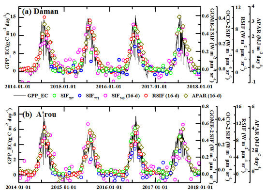
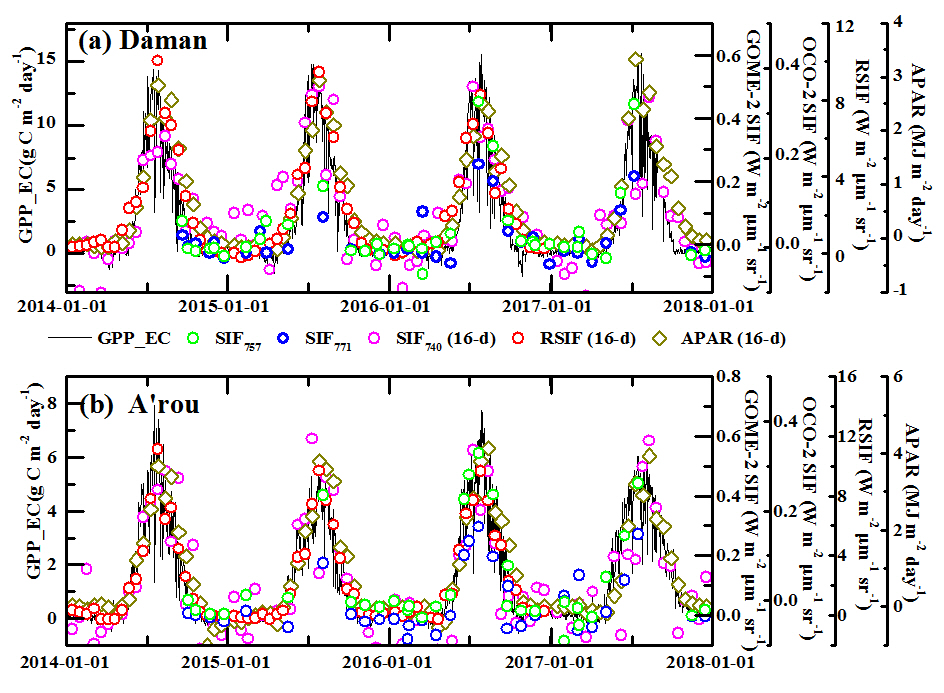
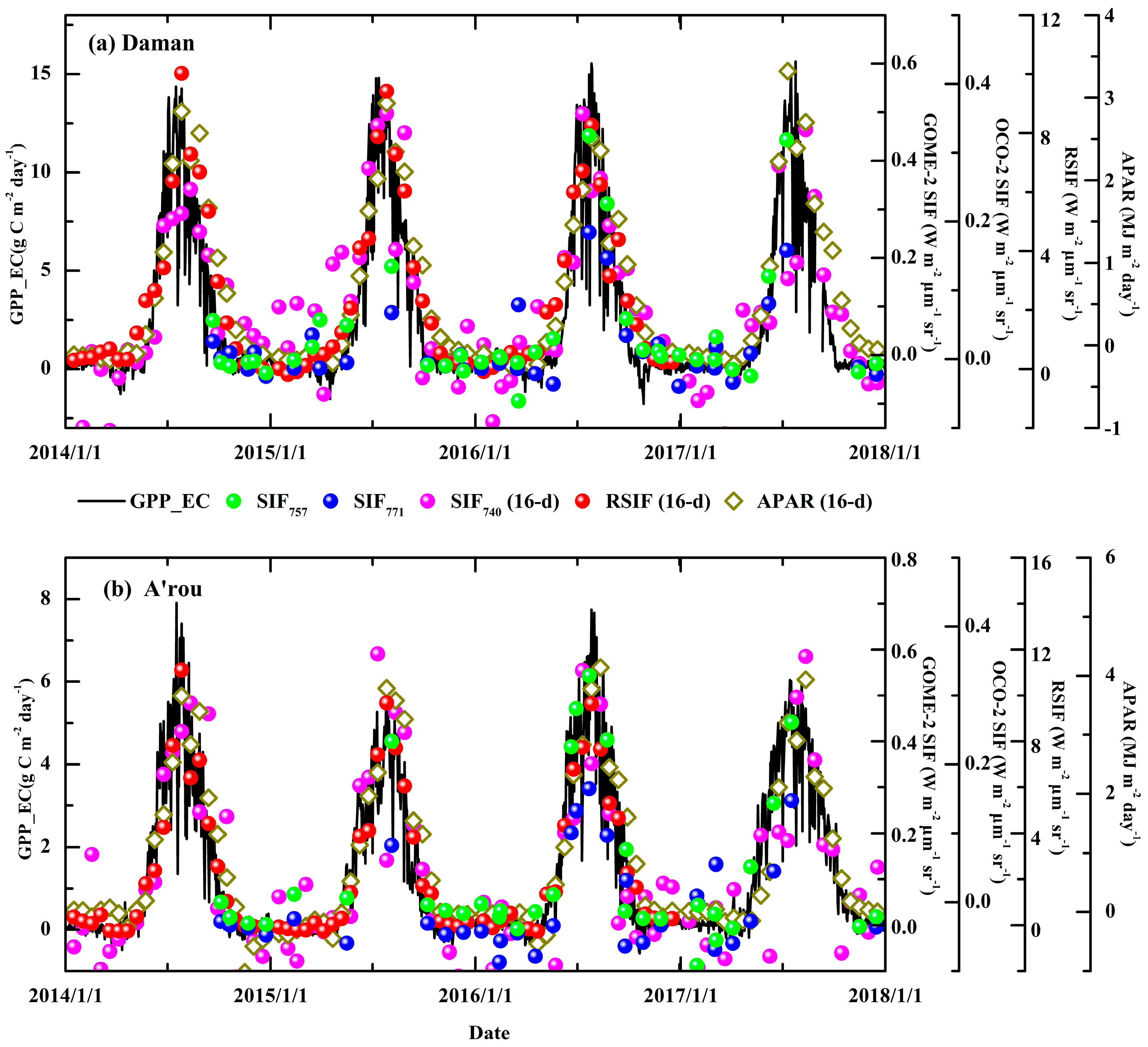
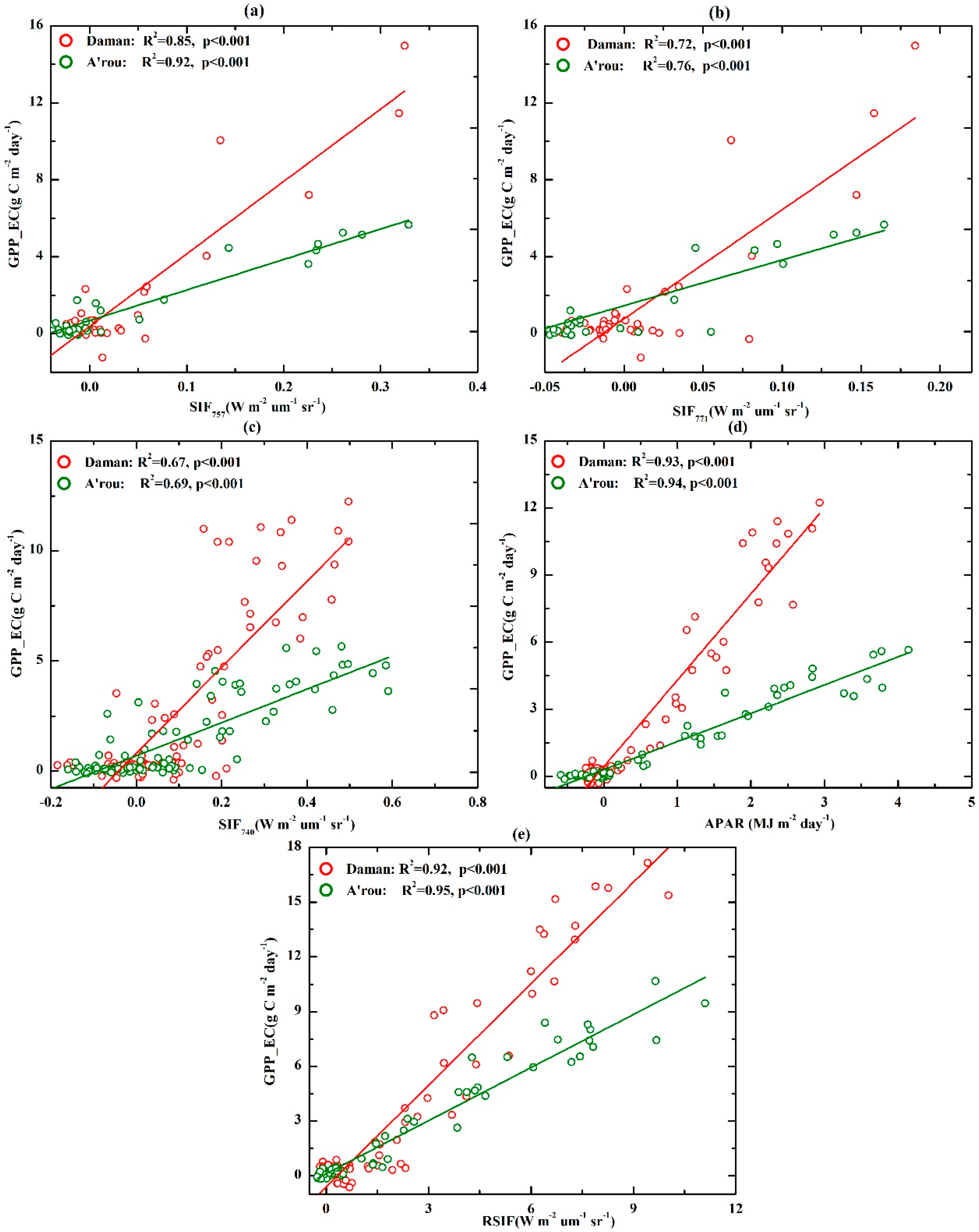
3.1. Relationships of SIF and APAR with Tower GPP

The seasonal dynamics of daily OCO-2 SIF, averaged APAR (16-d), GOME-2 SIF (16-d), RSIF (16-d), and daily tower GPP for the Daman and A’rou sites from 2014–2017 are shown in Figure 2. APAR was calculated by Equation (4). The variations in SIF₇₅₇, SIF₇₇₁, SIF₇₄₀, RSIF, and APAR exhibited seasonal patterns that were similar to those of the tower GPP at both sites. SIF₇₅₇, SIF₇₇₁, SIF₇₄₀, RSIF, and APAR showed large discrepancies from the tower GPP measurements during the spring onset, the peak of the growing season and senescence stages, and the tower GPP reflected slightly better consistency with SIF₇₅₇, RSIF and APAR than with SIF₇₇₁ and SIF₇₄₀.

As shown in Figure 3, OCO-2 SIF₇₅₇ and SIF₇₇₁ showed much stronger linear correlations with the tower GPP at a daily timescale than shown by GOME-2 SIF₇₄₀ and tower GPP at a 16-d averaged timescale. The goodness-of-fit between SIF₇₅₇ and tower GPP was better than that between SIF₇₇₁ and tower GPP at both sites (Daman and A’rou), and the goodness-of-fit between SIF₇₄₀ and tower GPP was relatively weak at a 16-d averaged timescale at both sites. The correlation between SIF₇₇₁ and tower GPP is weaker than the correlation between SIF₇₅₇ and tower GPP, but stronger than the correlation between SIF₇₄₀ and tower GPP. The 16-d averaged APAR and RSIF had the strongest linear correlations with 16-d averaged tower GPP. The correlations between SIF₇₅₇ and tower GPP, SIF₇₇₁ and tower GPP at a daily timescale were greater at the A’rou site than at the Daman site. So were correlations between SIF₇₄₀ and tower GPP, RSIF and tower GPP, APAR and tower GPP at a 16-d averaged timescale. In general, OCO2 SIF (SIF₇₅₇ and SIF₇₇₁), GOME-2 SIF, RSIF, and APAR showed strong relationships with tower GPP.

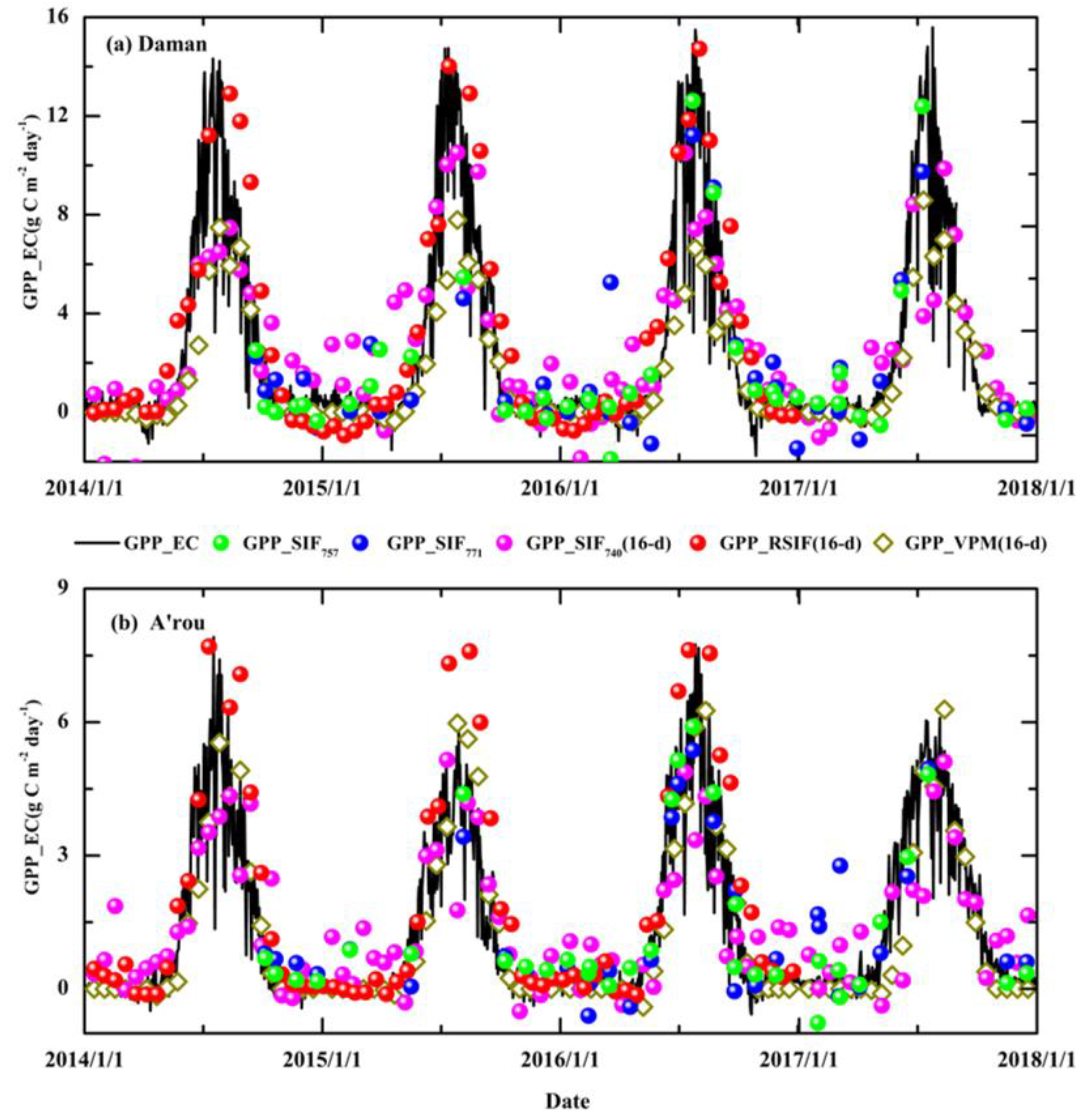
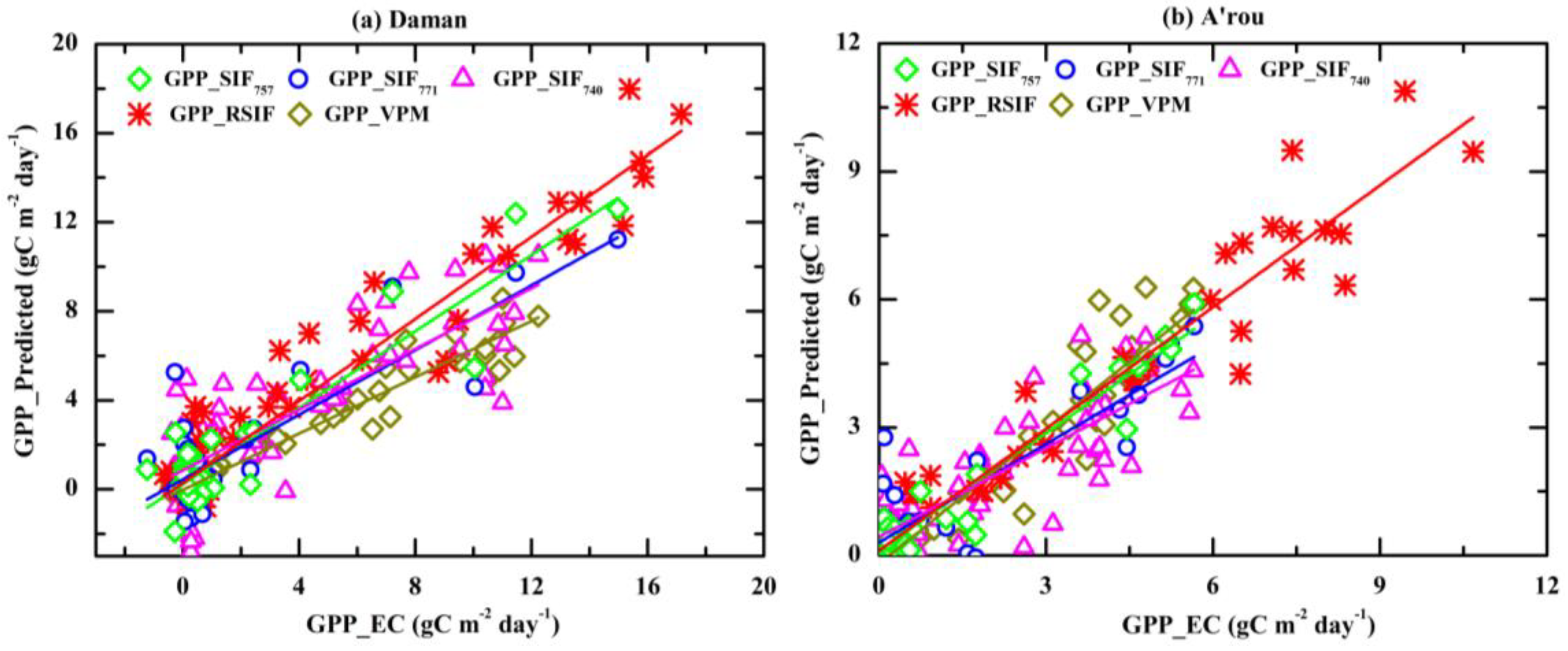
3.2. Evaluating the Performance of the GPP Estimates Based on Different Methods

The biome-specific (crop and grass) GPP-SIF relationships were obtained by fitting a linear function to the SIF and tower GPP at the Daman and A’rou sites (at Daman: GPP_SIF₇₅₇ = 37.63 × SIF₇₅₇ + 0.39, GPP_SIF₇₇₁ = 56.66 × SIF₇₇₁ + 0.77, GPP_SIF₇₄₀ = 19.50 × SIF₇₄₀ + 0.81, GPP_RSIF = 1.85 × RSIF − 0.59; at A’rou: GPP_SIF₇₅₇ = 15.86 × SIF₇₅₇ + 0.69, GPP_SIF₇₇₁ = 23.75 × SIF₇₇₁ + 1.46, GPP_SIF₇₄₀ = 7.54 × SIF₇₄₀ + 0.70, GPP_RSIF = 0.97 × RSIF + 0.12). The predicted GPP values based on SIF₇₅₇, SIF₇₇₁, SIF₇₄₀, RSIF, and VPM and the tower GPP are shown in Figure 4 and Figure 5. The GPP estimates from SIF₇₅₇, SIF₇₇₁, SIF₇₄₀, RSIF, and VPM effectively tracked the magnitude and seasonal dynamics of the tower GPP at the Daman and A’rou sites, especially RSIF, VPM, and SIF₇₅₇, which captured the beginning period, thriving period and end period of the growing season. In contrast, the SIF₇₇₁ and SIF₇₄₀-based model exhibited similarly weaker performances than other three models in predicting GPP. GPP_VPM and GPP_RSIF exhibited the best performance in GPP estimation, closely followed by GPP_SIF₇₅₇, then GPP_SIF₇₇₁ and GPP_SIF₇₄₀, while GPP_SIF₇₅₇ had the lowest RMSE among the models (Figure 5,

Table 2. Comparison between the tower GPP and model-predicted GPP.

		OCO-2		GPP_VPM (16-d)	GOME-2 (16-d)
		GPP_SIF757	GPP_SIF771		GPP_SIF740	GPP_RSIF
Daman	R2	0.86	0.72	0.95	0.68	0.92
	a	0.86	0.73	0.63	0.68	0.92
	b	0.23	0.45	−0.06	0.86	0.29
	p	<0.001	<0.001	<0.001	<0.001	<0.001
	RMSE	1.29	1.79	1.81	2.13	1.46
A’rou	R2	0.91	0.76	0.94	0.69	0.95
	a	0.92	0.77	1.05	0.7	0.95
	b	0.11	0.3	−0.19	0.43	0.11
	p	<0.001	<0.001	<0.001	<0.001	<0.001
	RMSE	0.52	0.88	0.54	0.98	0.67

¹ R² indicates the determination coefficient, and a and b represent the slope and intercept of the linear regression.

). The correlation coefficients between GPP predicted by the SIF (SIF₇₅₇, SIF₇₇₁, SIF₇₄₀, and RSIF) and tower GPP, and GPP predicted by VPM model and tower GPP were greater at the A’rou site than at the Daman site.

3.3. Possible Reasons for the Differences Among the OCO-2, GOME-2 and Flux Tower GPPs

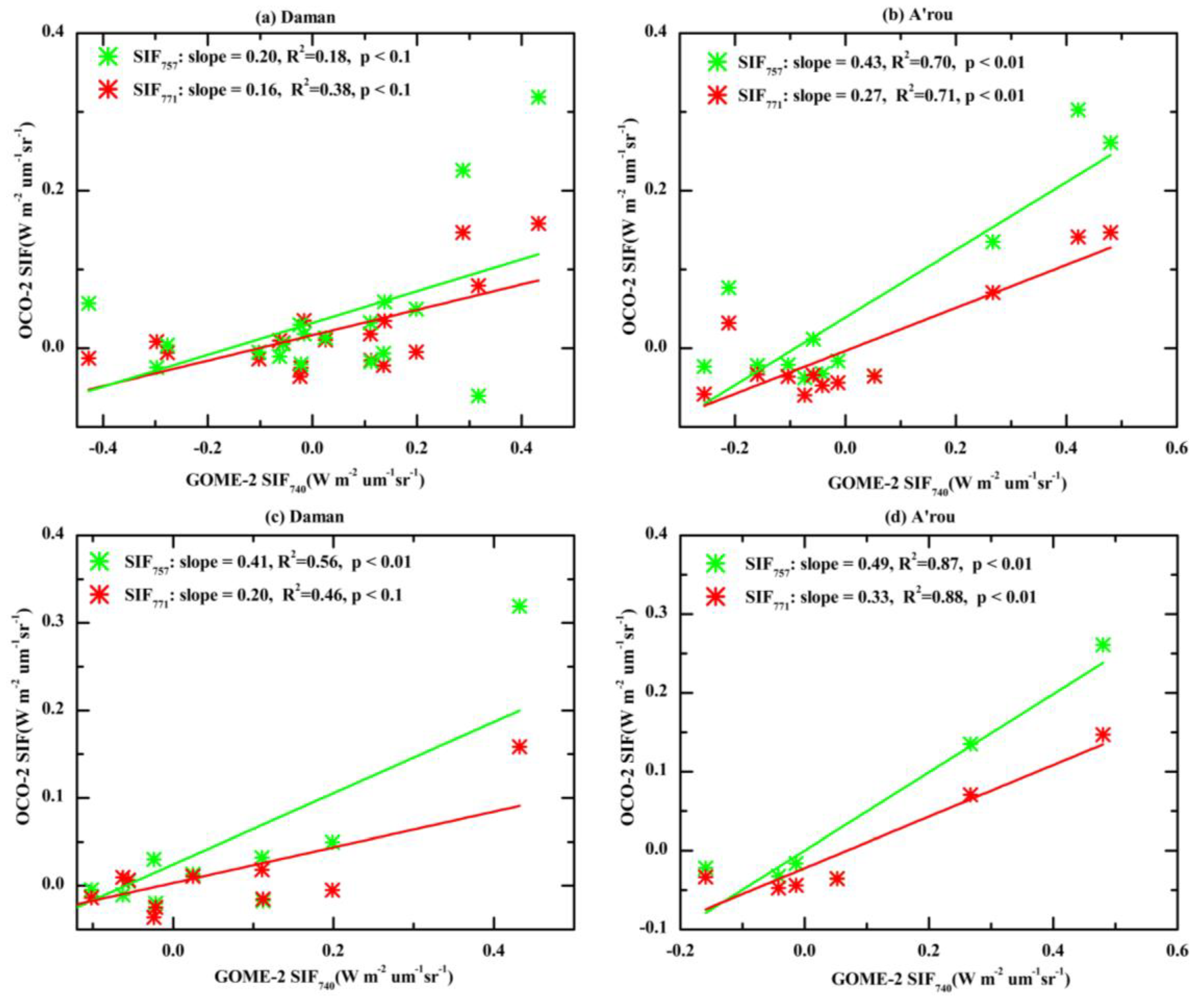
3.3.1. Effects of Spatial Mismatches on the Differences Among the OCO-2 SIF, GOME-2 SIF, and Flux Tower GPPs

In this study, we demonstrated the correlation between OCO-2 SIF and tower GPP was stronger than the correlation between GOME-2 SIF with tower GPP. One of the reasons for this discrepancy is the spatial mismatch between the GOME-2 and OCO-2 footprints (Figure 6). A 0.5° grid cell around the flux site was used to extract GOME-2 and OCO-2 data. Within the grid cell, OCO-2 data covered only a narrow strip, while GOME-2 pixels covered the majority of the grid cell and were more or less outside the grid cell. For OCO-2 or GOME-2, the pixels located within the 0.5° grid cell changed over time. Due to different revisit periods, the overlap area changed greatly with time and location. A spatial overlap was observed between the GOME-2 and OCO-2 footprints and a given 0.5° grid cell based on the coordinates of each flux tower for samples on the corresponding date. For certain days, the GOME-2 SIF had high spatial overlaps with the OCO-2 SIF, such as on 17 May 2015, 13 February 2016, 26 October 2016, and 5 March 2017 at the Daman site as well as 21 October 2014, 24 December 2014, 6 December 2014, 18 July 2017, and 16 November 2017 at the A’rou site. However, the size of the spatial overlap was very small on other dates, such as on 6 September 2015 and 26 September 2016 at Daman and 31 July 2016 and 5 March 2017 at A’rou (Figure 6, Figures S4 and S5). The correlation between GOME-2 SIF and OCO-2 SIF was dependent on the size of the overlap, which may result in differences between OCO-2 SIF and GOME-2 SIF.

The GOME-2 SIF was compared with the OCO-2 SIF based on all soundings and the soundings with numbers greater than 70 at a daily timescale; then, how the sizes of the spatial overlaps influenced the OCO-2 SIF and GOME-2 SIF relationship was examined (Figure 7, Figures S4 and S5). We found that the correlation coefficients between GOME-2 SIF and OCO-2 SIF based on samples with more than 70 soundings were stronger than the correlation coefficients between GOME-2 SIF and OCO-2 SIF based on all soundings at both the Daman and A’rou sites. Correspondingly, the slope also significantly varied with the sounding samples (i.e., the slopes increased obviously when the sample overlaps were based on more than 70 soundings). This analysis indicated that the robustness of the correlation coefficients between GOME-2 SIF and OCO-2 SIF was highly dependent on their spatial overlaps.

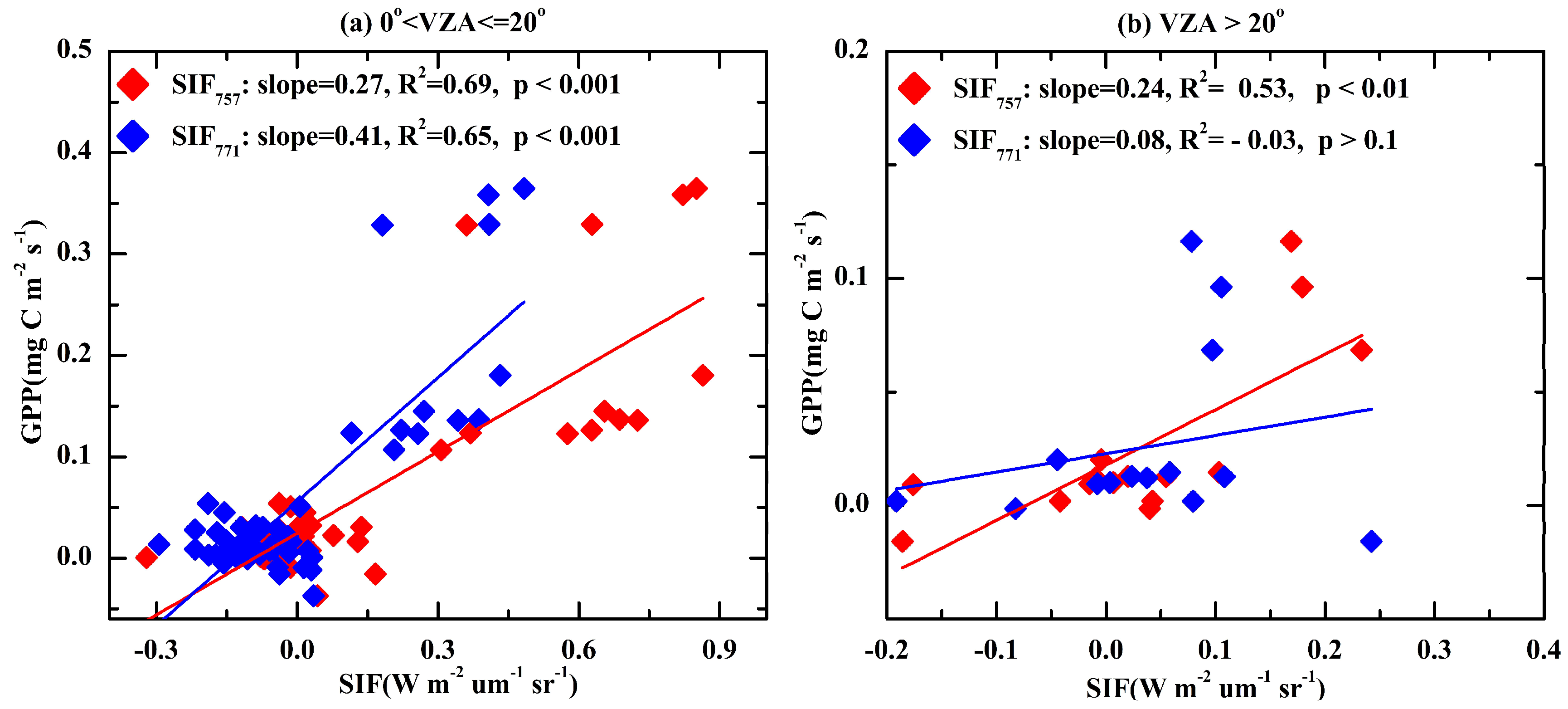
3.3.2. Effects of the Viewing Zenith Angle (VZA) on the Relationship Between SIF and Tower GPP

We compared the OCO-2 instantaneous SIF averages based on all soundings of the VZA intervals to investigate whether the VZA had an impact on the GPP-SIF relationship (Figure 8). Due to the sparse coverage of OCO-2, the number of OCO-2 SIF samples was limited, with 71 samples obtained for the Daman and A’rou sites combined. The VZA values were divided into two intervals: 0° < VZA ≤ 20° (the number of OCO-2 SIF samples was 56; most of them were in the nadir mode); VZA > 20° (the number of OCO-2 SIF samples was 15; all were in the glint mode). The results showed that SIF₇₅₇ and SIF₇₇₁ in the interval of 0° < VZA ≤ 20° showed a stronger correlation with the tower GPP than SIF₇₅₇ and SIF₇₇₁ in the interval of VZA > 20° at an instantaneous timescale. The averaged SIF and the slope with 0°< VZA ≤20° exhibited slightly higher values than those with VZA > 20°, and the statistical significance was more evident in the interval of 0°< VZA ≤ 20° than in the interval of VZA > 20° (Figure 8). OCO-2 SIF obtained by the sensor in the nadir mode performed better than that obtained in the glint mode. OCO-2 SIF was highly sensitive to the VZA, and the VZA might play an important role in the GPP-SIF relationship.

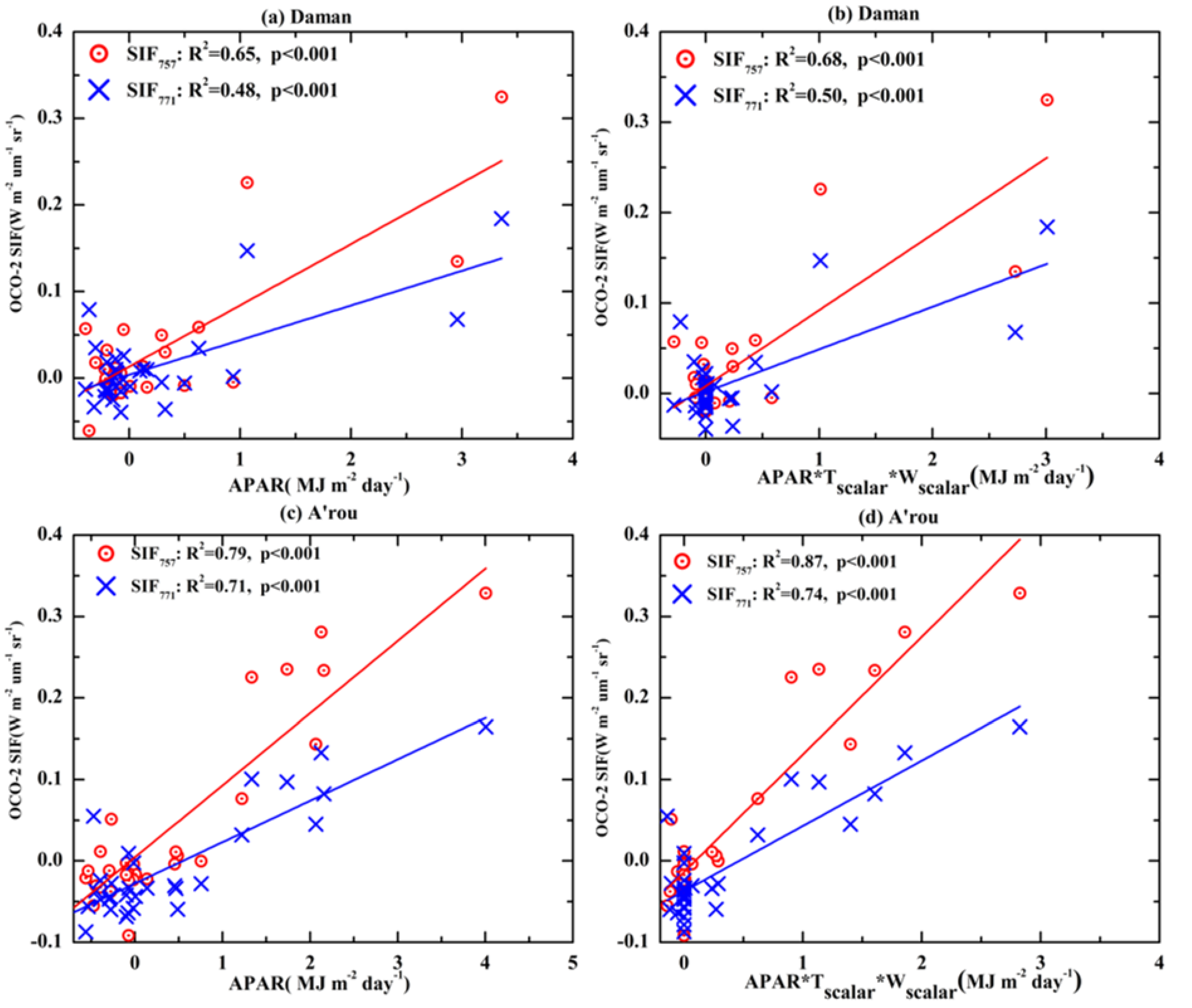
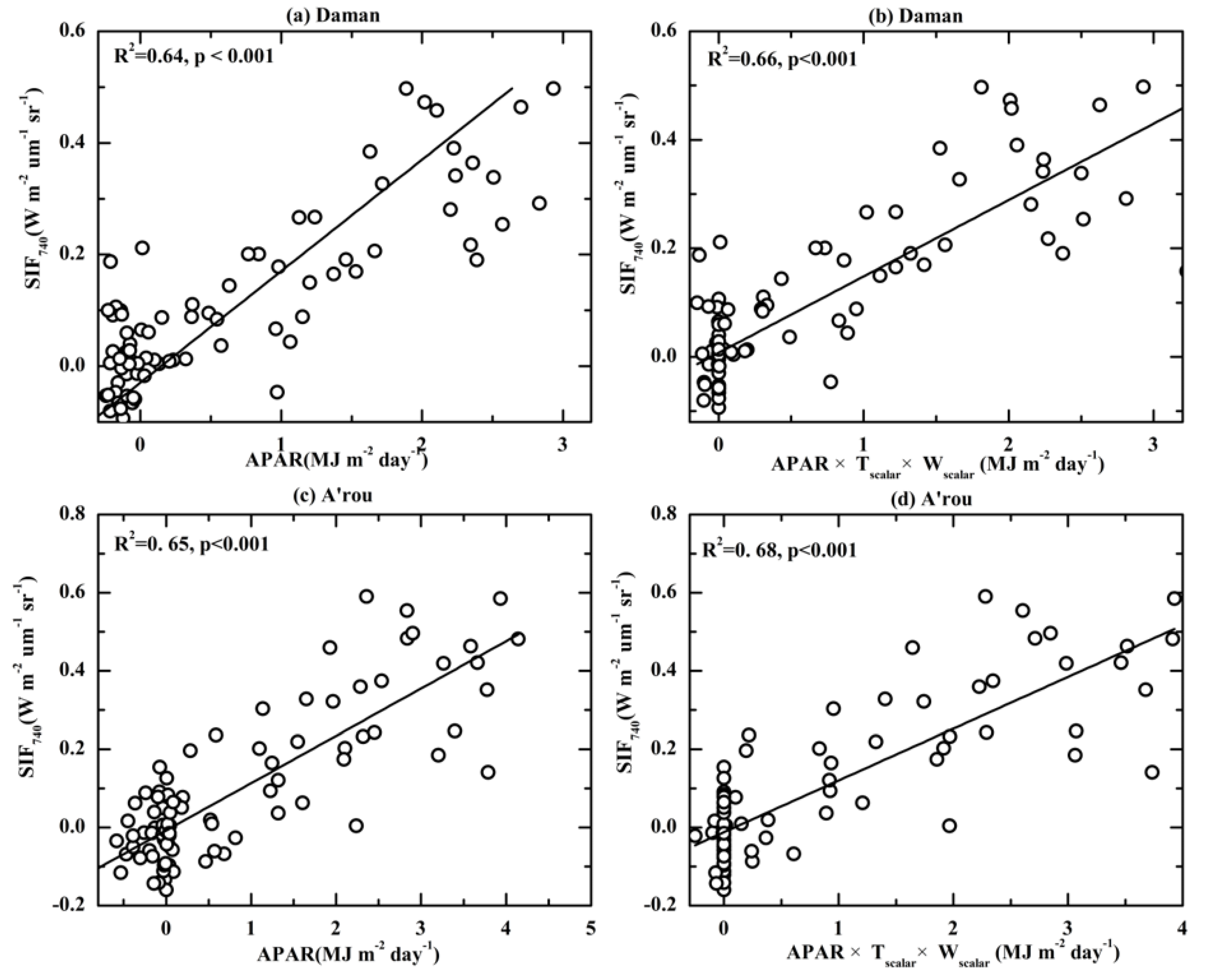
3.3.3. Relationships of the OCO-2 and GOME-2 SIF with APAR and APAR × T_scalar × W_scalar

At the Daman site, APAR and APAR × T_scalar × W_scalar explained 65% and 68% of the variance in SIF₇₅₇ as well as 48% and 50% of the variance in SIF₇₇₁, respectively (Figure 9a,b). At the A’rou site, APAR and APAR × T_scalar × W_scalar explained 79% and 87% of the variance in SIF₇₅₇ as well as 71% and 74% of the variance in SIF₇₇₁, respectively (Figure 10c,d). The correlations were much higher at A’rou than at Daman. These results indicated that both SIF₇₅₇ and SIF₇₇₁ were mainly dependent on APAR. APAR and the two environmental scaling factors (APAR × T_scalar × W_scalar) accounted for more variance in SIF₇₅₇ and SIF₇₇₁ than APAR accounted for alone at both sites, which indicates that both SIF₇₅₇ and SIF₇₇₁ were also related to environmental stresses.

At the Daman site, APAR and APAR × T_scalar × W_scalar explained 64% and 66% of the variance in SIF₇₄₀ as well as 65% and 68% of the variance in SIF₇₄₀ at the A’rou site, respectively (Figure 10). The correlations of SIF₇₄₀ with APAR and APAR × T_scalar × W_scalar were higher at the A’rou site than that at the Daman site, which was similar to the results of OCO-2 SIF. In contrast, the correlation of SIF₇₄₀ with APAR × T_scalar × W_scalar was higher than the correlation with APAR alone. These results indicated that SIF₇₄₀ was also affected by APAR and relevant to the two environmental scaling factors (T_scalar × W_scalar).

4. Discussion

Recent studies have shown that satellite-based SIF retrieval is a powerful method for monitoring vegetation dynamics and estimating GPP at regional and global scales, and the findings of these studies indicated that SIF-based GPP models perform better than the traditional state-of-the-art carbon cycle models in cropland, grassland, and forests [24,33,31,35,55,61]. However, comparative studies using SIF obtained from OCO-2 SIF and GOME-2 to estimate GPP for multiple cropping and grass areas were insufficient in previous studies, especially for cold and arid areas of China. In this study, we evaluated the performance of SIF obtained by OCO-2 and GOME-2 for GPP estimation in the Heihe River Basin, China.

We demonstrated that OCO-2 SIF₇₅₇, SIF₇₇₁, GOME-2 SIF₇₄₀, RSIF, and APAR captured seasonal dynamics well in maize and alpine meadow, especially RSIF, APAR, and SIF₇₅₇. Similarly, GPP_VPM and GPP_RSIF had strong relationships with GPP_EC and they performed best in predicting GPP, followed by GPP_SIF₇₅₇ model, then GPP_SIF₇₇₁ and GPP_SIF₇₄₀. The GOME-2 observations used in our study were noisy, they were collected at various viewing angles, under various cloud conditions, and at different locations. RSIF was developed based on MODIS reflectance inputs, and it has a large improvement than the original GOME-2 SIF. As the MODIS data are less noisy than the original GOME-2 product, the far-red GOME-2 SIF largely reflect changes in APAR absorbed by chlorophyll. Additionally, if only the single OCO-2 observation closest to the tower was used for comparison, it would probably be similarly noisy; if the OCO-2 SIF observations were spatially averaged, the average values would result in the degradation of the original resolution and the reduction of noise. Therefore, there is always a tradeoff with satellite data, e.g., spatial vs. spectral resolution or spatial vs. temporal resolution. GPP_VPM performed very well, because VPM was calculated from APAR, which is the product of fPAR and PAR, and fPAR accounted for a nonzero background and provided a mean value of scaling the otherwise unquantified EVI [11,62]. Moreover, most parameters of VPM covered the total area of the 0.5° grid cell; OCO-2 SIF₇₅₇ and SIF₇₇₁ covered narrow strips, which only partially captured the signal of the grid cell, and the GOME-2 pixels covered the majority of the 0.5°grid cell. In previous studies, GOME-2 SIF retrievals were averaged to 8-d, 16-d, or monthly under the condition that at least five SIF retrievals were available [24,33,42,63]. GOME-2 SIF performed well in GPP estimation; this strong performance was further confirmed in our study. Compared to OCO-2 average, GOME-2 SIF average (16-d) exhibited a general performance in GPP estimation, due to the coarse spatial resolution of the data. The spatial resolution and quality of the OCO-2 SIF data are greater than GOME-2 SIF data [44,64]. The correlation coefficients between GPP predicted by the SIF (SIF₇₅₇, SIF₇₇₁, SIF₇₄₀, and RSIF) and tower GPP, and GPP predicted by VPM model and tower GPP were greater at the A’rou site than at the Daman site. Because Daman is more heterogeneous than A’rou, and the ecosystem in Daman is highly heterogeneous at spatial scales larger than 10 km [37,65,66]. Several recent studies reported that OCO-2 SIF had strong correlation coefficients with tower GPP in crop, grassland, and temperate forest areas [31,34,35], our results were consistent with these conclusions.

We performed an intercomparison using OCO-2 SIF to verify the GOME-2 SIF results and found that the spatial differences in the footprints among GOME-2, OCO-2 and the flux towers represented one of the main reasons for the large discrepancies in the GPP estimates. We found that the robustness of the correlation coefficients between GOME-2 SIF and OCO-2 SIF were highly dependent on their spatial footprint overlaps, which might be one of the reasons why GOME-2 SIF exhibited universal correlation with the tower GPP. GOME-2 SIF showed stronger correlation coefficients with OCO-2 SIF based on samples with more than 70 soundings than with OCO-2 SIF based on all soundings (Figure 7, Figures S4 and S5), because SIF retrieval with less than 70 soundings within the spatial footprint overlaps could increase the effects of potential noise in the retrievals. The OCO-2 scale effect could demonstrate this phenomenon to some extent (Figure S1, Table S1), and when averaging in different bins, additional soundings were sorted into larger bins, which could reduce the effects of retrieval noise. Thus, OCO-2 SIF manifested a stronger correlation with the tower GPP. For GOME-2 SIF, the scale effect was weaker than the results of OCO-2 SIF (Figure S2, Table S1). We examined the daily GOME-2 observations and found them to be noisy; thus, we averaged them over time to reduce noise in a similar way as OCO-2 data were averaged in space.

Our results demonstrated that OCO-2 SIF obtained by the sensor observing the surface in the nadir mode performed better than that obtained by the sensor in the direct sunlight reflected in the glint mode, because in the nadir mode, the satellite points the instrument to the local nadir with zero VZAs. In the glint mode, noticeable angular variations of SIF exist due to the varying VZA over time, and major directional effects on SIF added variations of the GPP-SIF relationship and OCO-2 SIF values [29,67,68].

Our results also showed that the OCO-2 SIF and GOME-2 SIF were correlated with APAR as well as with two environmental scaling factors (T_scalar × W_scalar). These findings were consistent with previous studies [22,31]. Different variables, such as EVI, PAR, air temperature, and LSWI, as well as a set of biome-specific parameters (e.g., maximum LUE, maximum, minimum, and optimum temperature) are included in the VPM model; SIF-based models such as linear models use a simple computational process for GPP estimations. However, it is unclear whether SIF-based models have lower uncertainties than VPM model in GPP estimation; this is a direction for future research. Besides, clouds could be a factor that influenced the SIF signals (Figure S3).

However, both OCO-2 SIF and GOME-2 SIF have certain limitations in GPP estimations. OCO-2 SIF has sparse coverage and low temporal resolution, and GOME-2 SIF has coarse spatial resolution [46,69], which severely hinders the investigations of the GPP-SIF relationship. Machine learning methods such as a feedforward neural networks architecture will provide an effective way to reproduce improved data [38], we expect a series of original issues such as sparse coverage and coarse spatial resolution will be improved to some extent. Importantly, we focus on space-borne SIF data with high spatiotemporal resolution. The tropospheric monitoring instrument (TROPOMI), on the Sentinel-5 Precursor platform, was launched on 16 August 2017, has a footprint size of 7 km × 7 km at nadir [70,71]. TanSat (CarbonSat) was launched on 21 December 2016 [72], which has a footprint size of approximately 2 km × 2 km and a swath of 20 km wide at nadir with a revisit period of 16 days. These space-borne datasets will be available to the public, when it can be further used for GPP estimation and the carbon cycle research.

5. Conclusions

In this study, we evaluated the performance of SIF obtained by OCO-2 and GOME-2 in the estimation of GPP for maize and alpine meadow areas at the Daman and A’rou sites. The main conclusions of this study are as follows.

The results showed that daily SIF₇₅₇ had stronger correlations with daily tower GPP than daily SIF₇₇₁, and the correlation between daily SIF_{757 and} daily tower GPP was stronger than the correlation between 16-d averaged SIF₇₄₀ and 16-d averaged tower GPP. The 16-d averaged APAR and RSIF had the strongest linear correlations with 16-d averaged tower GPP. GPP_VPM and GPP_RSIF exhibited the best performance in GPP estimation, closely followed by GPP_SIF₇₅₇, then GPP_SIF₇₇₁ and GPP_ SIF₇₄₀.

The robustness of the correlation coefficients of GOME-2 SIF with OCO-2 SIF was highly dependent on the size of the spatial footprint overlaps, indicating that the spatial differences between the GOME-2 and OCO-2 footprints and flux tower footprints played a role in explaining the differences in GPP estimates from towers and satellites. The scale effect of GOME-2 SIF was weaker than that of OCO-2 SIF on the SIF values and GPP-SIF relationships. Moreover, the VZA had a significant effect on the SIF values and the GPP-SIF relationships because directional effects on SIF added variations to the OCO-2 SIF observations. Our results showed that SIF was significantly correlated with APAR as well as environmental scalars (T_scalar × W_scalar).

References

1. Demmig-Adams, B.; Adams, W.W. Photosynthesis—Harvesting sunlight safely. Nature 2000, 403, 371–374. [Google Scholar] [CrossRef] [PubMed]
2. Ballantyne, A.P.; Alden, C.B.; Miller, J.B.; Tans, P.P.; White, J.W. Increase in observed net carbon dioxide uptake by land and oceans during the past 50 years. Nature 2012, 488, 70–72. [Google Scholar] [CrossRef]
3. Peters, W.; Jacobson, A.R.; Sweeney, C.; Andrews, A.E.; Conway, T.J.; Masarie, K.; Miller, J.; Bruhwiler, L.P.; Petron, G.; Hirsch, A.; et al. An atmospheric perspective on North American carbon dioxide exchange: Carbon tracker. Proc. Natl. Acad. Sci. USA 2007, 104, 18925–18930. [Google Scholar] [CrossRef] [PubMed]
4. Garbulsky, M.F.; Filella, I.; Verger, A.; Penuelas, J.; Filella, M.F. Photosynthetic light use efficiency from satellite sensors: From global to Mediterranean vegetation. Environ. Exp. Bot. 2014, 103, 3–11. [Google Scholar] [CrossRef]
5. Xiao, X.; Zhang, Q.; Braswell, B.; Urbanski, S.; Boles, S.; Wofsy, S.; Iii, B.M.; Ojima, D. Modeling gross primary production of temperate deciduous broadleaf forest using satellite images and climate data. Remote Sens. Environ. 2004, 91, 256–270. [Google Scholar] [CrossRef]
6. Running, S.W.; Nemani, R.R.; Heinsch, F.A.; Zhao, M.S.; Reeves, M.; Hashimoto, H. A continuous satellite-derived measure of global terrestrial primary production. Bioscience 2004, 54, 547–560. [Google Scholar] [CrossRef]
7. Potter, C.S.; Randerson, J.T.; Field, C.B.; Matson, P.A.; Vitousek, P.M.; Mooney, H.A.; Klooster, S.A. Terrestrial ecosystem production—A process model-based on global satellite and surface data. Glob. Biogeochem. Cycles 1993, 7, 811–841. [Google Scholar] [CrossRef]
8. Yuan, W.P.; Liu, S.; Zhou, G.S.; Zhou, G.Y.; Tieszen, L.L.; Baldocchi, D.; Bernhofer, C.; Gholz, H.; Goldstein, A.H.; Goulden, M.L.; et al. Deriving a light use efficiency model from eddy covariance flux data for predicting daily gross primary production across biomes. Agric. For. Meteorol. 2007, 143, 189–207. [Google Scholar] [CrossRef] [Green Version]
9. Grace, J.; Nichol, C.; Disney, M.; Lewis, P.; Quaife, T.; Bowyer, P. Can we measure terrestrial photosynthesis from space directly, using spectral reflectance and fluorescence? Glob. Chang. Biol. 2007, 13, 1484–1497. [Google Scholar] [CrossRef]
10. Haboudane, D.; Miller, J.R.; Pattey, E.; Zarco-Tejada, P.J.; Strachan, I. Hyperspectral vegetation indices and novel algorithms for predicting green LAI of crop canopies: Modeling and validation in the context of precision agriculture. Remote Sens. Environ. 2004, 90, 337–352. [Google Scholar] [CrossRef]
11. Li, X.; Xiao, J.; He, B.; Altaf, A.M.; Beringer, J.; Desai, A.R.; Emmel, C.; Hollinger, D.Y.; Krasnova, A.; Mammarella, I.; et al. Solar-induced chlorophyll fluorescence is strongly correlated with terrestrial photosynthesis for a wide variety of biomes: First global analysis based on OCO-2 and flux tower observations. Glob. Chang. Biol. 2018, 24, 3990–4008. [Google Scholar] [CrossRef] [PubMed]
12. Dobrowski, S.Z.; Pusknik, J.C.; Zarco-Tejada, P.J.; Ustin, S.L. Simple reflectance indices track heat and water stress induced changes in steady state chlorophyll fluorescence. Remote Sens. Environ. 2005, 97, 403–414. [Google Scholar] [CrossRef]
13. Zhao, M.; Running, S.W.; Nemani, R.R. Sensitivity of moderate resolution imaging spectroradiometer (MODIS) terrestrial primary production to the accuracy of meteorological reanalyses. J. Geophys. Res. Biogeosci. 2006, 111, G01002. [Google Scholar] [CrossRef]
14. Tramontana, G.; Jung, M.; Schwalm, C.R.; Ichii, K.; Campsvalls, G.; Ráduly, B.; Reichstein, M.; Arain, M.A.; Cescatti, A.; Kiely, G.; et al. Predicting carbon dioxide and energy fluxes across global fluxnet sites with regression algorithms. Biogeoscience 2016, 13, 4291–4313. [Google Scholar] [CrossRef]
15. Jung, M.; Tautenhahn, S.; Wirth, C.; Kattge, J. Estimating basal area of spruce and fir in post-fire residual stands in central siberia using quickbird, feature selection, and random forests. Procedia Comput. Sci. 2013, 18, 2386–2395. [Google Scholar] [CrossRef]
16. Guan, K.Y.; Berry, J.A.; Zhang, Y.G.; Joiner, J.; Guanter, L.; Badgley, G.; Lobell, D.B. Improving the monitoring of crop productivity using spaceborne solar-induced fluorescence. Glob. Chang. Biol. 2016, 22, 716–726. [Google Scholar] [CrossRef]
17. Liu, X.J.; Guanter, L.; Liu, L.Y.; Damm, A.; Malenovský, Z.; Rascher, U.; Peng, D.L.; Du, S.S.; Gastellu-Etchegorry, J.P. Downscaling of solar-induced chlorophyll fluorescence from canopy level to photosystem level using a random forest model. Remote Sens. Environ. 2018, 5. [Google Scholar] [CrossRef]
18. Zhang, Y.G.; Guanter, L.; Joiner, Jo.; Song, L.; Guan, K.Y. Spatially-explicit monitoring of crop photosynthetic capacity through the use of space-based chlorophyll fluorescence data. Remote Sens. Environ. 2018, 210, 362–374. [Google Scholar] [CrossRef]
19. Baker, N.R. Chlorophyll fluorescence: A probe of photosynthesis in vivo. Ann. Rev. Plant Biol. 2008, 59, 89–113. [Google Scholar] [CrossRef]
20. Porcar-Castell, A.; Tyystjarvi, E.; Atherton, J.; Van der Tol, C.; Flexas, J.; Pfundel, E.E.; Moreno, J.; Frankenberg, C.; Berry, J.A. Linking chlorophyll a fluorescence to photosynthesis for remote sensing applications: Mechanisms and challenges. J. Exp. Bot. 2014, 65, 4065–4095. [Google Scholar] [CrossRef]
21. Lee, J.E.; Berry, J.A.; Van der Tol, C.; Yang, X.; Guanter, L.; Damm, A.; Baker, I.; Frankenberg, C. Simulations of chlorophyll fluorescence incorporated into the Community Land Model version 4. Glob. Chang. Biol. 2015, 21, 3469–3477. [Google Scholar] [CrossRef] [PubMed] [Green Version]
22. Yang, X.; Tang, J.W.; Mustard, J.F.; Lee, J.E.; Rossini, M.; Joiner, J.; Munger, J.W.; Kornfeld, A.; Richardson, A.D. Solar-induced chlorophyll fluorescence that correlates with canopy photosynthesis on diurnal and seasonal scales in a temperate deciduous forest. Geophys. Res. Lett. 2015, 42, 2977–2987. [Google Scholar] [CrossRef] [Green Version]
23. Rossini, M.; Nedbal, L.; Guanter, L.; Ac, A.; Alonso, L.; Burkart, A.; Cogliati, S.; Colombo, R.; Damm, A.; Drusch, M.; et al. Red and far red sun-induced chlorophyll fluorescence as a measure of plant photosynthesis. Geophys. Res. Lett. 2015, 42, 1632–1639. [Google Scholar] [CrossRef]
24. Wagle, P.; Zhang, Y.; Jin, C.; Xiao, X. Comparison of solar-induced chlorophyll fluorescence, light-use efficiency, and process-based GPP models in maize. Ecol. Appl. 2016, 26, 1211–1222. [Google Scholar] [CrossRef] [PubMed]
25. Frankenberg, C.; O’Dell, C.; Berry, J.; Guanter, L.; Joiner, J.; Kohler, P.; Pollock, R.; Taylor, T.E. Prospects for chlorophyll fluorescence remote sensing from the orbiting carbon observatory-2. Remote Sens. Environ. 2014, 147, 1–12. [Google Scholar] [CrossRef]
26. Zhang, Y.G.; Guanter, L.; Berry, J.A.; Joiner, J.; van der Tol, C.; Huete, A.; Gitelson, A.; Voigt, M.; Kohler, P. Estimation of vegetation photosynthetic capacity from space-based measurements of chlorophyll fluorescence for terrestrial biosphere models. Glob. Chang. Biol. 2014, 20, 3727–3742. [Google Scholar] [CrossRef] [Green Version]
27. Zhang, Y.; Xiao, X.M.; Jin, C.; Dong, J.W.; Zhou, S.; Wagle, P.; Joiner, J.; Guanter, L.; Zhang, Y.G.; Zhang, G.L.; et al. Consistency between sun-induced chlorophyll fluorescence and gross primary production of vegetation in North America. Remote Sens. Environ. 2016, 183, 154–169. [Google Scholar] [CrossRef] [Green Version]
28. Shiga, Y.P.; Tadić, J.M.; Qiu, X.M.; Yadav, V.; Andrews, A.E.; Berry, J.A.; Michalak, A.M. Atmospheric CO2 observations reveal strong correlation between regional net biospheric carbon uptake and solar-induced chlorophyll fluorescence. Geophys. Res. Lett. 2018, 45, 1122–1132. [Google Scholar] [CrossRef]
29. He, L.M.; Chen, J.M.; Liu, J.; Mo, G.; Joiner, J. Angular normalization of GOME-2 Sun-induced chlorophyll fluorescence observation as a better proxy of vegetation productivity. Geophys. Res. Lett. 2017, 44, 5691–5699. [Google Scholar] [CrossRef]
30. Jeong, S.J.; Schimel, D.; Frankenberg, C.; Drewry, D.T.; Fisher, J.B.; Verma, M.; Berry, J.A.; Lee, J.; Joiner, J. Application of satellite solar-induced chlorophyll fluorescence to understanding large-Scale variations in vegetation phenology and function over Northern high latitude forests. Remote Sens. Environ. 2017, 190, 178–187. [Google Scholar] [CrossRef]
31. Li, X.; Xiao, J.; He, B. Chlorophyll fluorescence observed by OCO-2 is strongly related to gross primary productivity estimated from flux towers in temperate forests. Remote Sens. Environ. 2018, 204, 659–671. [Google Scholar] [CrossRef]
32. Smith, W.K.; Biederman, J.A.; Scott, R.L.; Moore, D.J.P.; He, M.; Kimball, J.S.; Yan, D.; Hudson, A.; Barnes, M.L.; MacBean, N.; et al. Chlorophyll fluorescence better captures seasonal and interannual gross primary productivity dynamics across dryland ecosystems of Southwestern North America. Geophys. Res. Lett. 2018, 45, 748–757. [Google Scholar] [CrossRef]
33. Guanter, L.; Zhang, Y.; Jung, M.; Joiner, J.; Voigt, M.; Berry, J.A.; Frankenberg, C.; Huete, A.R.; Zarco-Tejada, P.; Lee, J.E.; et al. Global and time-resolved monitoring of crop photosynthesis with chlorophyll fluorescence. Proc. Natl. Acad. Sci. USA 2014, 111, E1327–E1333. [Google Scholar] [CrossRef] [PubMed] [Green Version]
34. Wood, J.D.; Griffis, T.J.; Baker, J.M.; Frankenberg, C.; Verma, M.; Yuen, K. Multiscale analyses of solar-induced florescence and gross primary production. Geophys. Res. Lett. 2017, 44, 533–541. [Google Scholar] [CrossRef]
35. Verma, M.; Schimel, D.; Evans, B.; Frankenberg, C.; Beringer, J.; Darren, D.T.; Magney, T.; Marang, I.; Hutley, L.; Moore, C.; et al. Effect of environmental conditions on the relationship between solar-induced fuorescence and gross primary productivity at an OzFlux grassland site. J. Geophys. Res.-Biogeosci. 2017, 122, 716–733. [Google Scholar] [CrossRef]
36. Frankenberg, C.; Fisher, J.B.; Worden, J.; Badgley, G.; Saatchi, S.S.; Lee, J.E.; Toon, G.C.; Butz, A.; Jung, M.; Kuze, A.; et al. New global observations of the terrestrial carbon cycle from GOSAT: Patterns of plant fluorescence with gross primary productivity. Geophys. Res. Lett. 2011, 38, L17706. [Google Scholar] [CrossRef]
37. Duveiller, G.; Cescatti, A. Spatially downscaling sun-induced chlorophyll fluorescence leads to an improved temporal correlation with gross primary productivity. Remote Sens. Environ. 2016, 182, 72–89. [Google Scholar] [CrossRef]
38. Gentine, P.; Alemohammad, S.H. Reconstructed solar-induced fluorescence: A machine learning vegetation product based on MODIS surface reflectance to reproduce GOME-2 solar-induced fluorescence. Geophys. Res. Lett. 2018, 45, 3136–3146. [Google Scholar] [CrossRef]
39. Li, X.; Cheng, G.D.; Liu, S.M.; Xiao, Q.; Ma, M.G.; Jin, R.; Che, T.; Liu, Q.H.; Wang, W.Z.; Qi, Y.; et al. Heihe watershed allied telemetry experimental research (HiWATER): Scientific objectives and experimental design. Bull. Am. Meteorol. Soc. 2013, 94, 1145–1160. [Google Scholar] [CrossRef]
40. Liu, S.M.; Xu, Z.W.; Zhu, Z.L.; Jia, Z.Z.; Zhu, M.J. Measurements of evapotranspiration from eddy-covariance systems and large aperture scintillometers in the Hai River Basin, China. J. Hydrol. 2013, 487, 24–38. [Google Scholar] [CrossRef]
41. Wang, X.F.; Cheng, G.D.; Li, X.; Lu, L.; Ma, M.G. An algorithm for gross primary production (GPP) and net ecosystem production (NEP) estimations in the midstream of the Heihe River Basin, China. Remote Sens. 2015, 7, 3651–3669. [Google Scholar] [CrossRef]
42. Sun, Y.; Frankenberg, C.; Wood, J.D.; Schimel, D.S.; Jung, M.; Guanter, L.; Drewry, D.T.; Verma, M.; Porcar-Castell, A.; Griffis, T.J.; et al. OCO-2 advances photosynthesis observation from space via solar-induced chlorophyll fluorescence. Science 2017, 358. [Google Scholar] [CrossRef] [PubMed]
43. Sun, Y.; Frankenberg, C.; Jung, M.; Joiner, J.; Guanter, L.; Köhler, P.; Magney, T. Overview of solar-induced chlorophyll fluorescence (SIF) from the Orbiting Carbon Observatory-2: Retrieval, cross-mission comparison, and global monitoring for GPP. Remote Sens. Environ. 2018, 209, 808–823. [Google Scholar] [CrossRef]
44. Ji, G.L.; Ma, X.Y.; Zou, J.L.; Liu, L.Z. Characteristics of the photosynthetically active radiation over Zhangye region. Plateau Meteorol. 1993, 12, 141–146. (In Chinese) [Google Scholar]
45. Li, Y.N.; Zhou, H.K. Features of photosynthetic active radiation (PAR) in Haibei alpine meadow area of Qilian mountain during plant growing period. Plateau Meteorol. 2002, 21, 9022. [Google Scholar]
46. Joiner, J.; Guanter, L.; Lindstrot, R.; Voigt, M.; Vasilkov, A.P.; Middleton, E.M.; Huemmrich, K.F.; Yoshida, Y.; Frankenberg, C. Global monitoring of terrestrial chlorophyll fluorescence from moderate-spectral-resolution near-infrared satellite measurements: Methodology, simulations, and application to GOME-2. Atmos. Meas. Tech. 2013, 6, 2803–2823. [Google Scholar] [CrossRef]
47. Joiner, J.; Yoshida, Y.; Guanter, L.; Middleton, E.M. New methods for the retrieval of chlorophyll red fluorescence from hyperspectral satellite instruments: Simulations and application to GOME-2 and SCIAMACHY. Atmos. Meas. Tech. 2016, 9, 3939–3967. [Google Scholar] [CrossRef]
48. Joiner, J.; Yoshida, Y.; Vasilkov, A.; Schaefer, K.; Jung, M.; Guanter, L.; Zhang, Y.; Garrity, S.; Middleton, E.M.; Huemmrich, K.F.; et al. The seasonal cycle of satellite chlorophyll fluorescence observations and its relationship to vegetation phenology and ecosystem atmosphere carbon exchange. Remote Sens. Environ. 2014, 152, 375–391. [Google Scholar] [CrossRef] [Green Version]
49. Wang, X.F.; Ma, M.G.; Huang, G.H.; Veroustraete, F.; Zhang, Z.H.; Song, Y.; Tan, J.L. Vegetation Primary Production Estimation at Maize and Alpine Meadow over the Heihe River Basin, China. Int. J. Appl. Earth Obs. Geoinf. 2012, 17, 94–101. [Google Scholar] [CrossRef]
50. Ruimy, A.; Jarvis, P.G.; Baldocchi, D.D.; Saugier, B. CO2 fluxes over plant canopies and solar radiation: A review. Adv. Ecol. Res. 1995, 26, 1–68. [Google Scholar]
51. Yan, H.M.; Fu, Y.L.; Xiao, X.M.; Huang, H.Q.; He, H.L.; Ediger, L. Modeling gross primary productivity for winter wheat-maize double cropping system using MODIS time series and CO2 eddy flux tower data. Agric. Ecosyst. Environ. 2009, 129, 391–400. [Google Scholar] [CrossRef]
52. Raich, J.W.; Rastetter, E.B.; Melillo, J.M.; Kicklighter, D.W.; Steudler, P.A.; Peterson, B.J.; Grace, A.L.; Moore, B.; Vorosmarty, C.J. Potential net primary productivity in south-America—Application of a global-model. Ecol. Appl. 1991, 1, 399–429. [Google Scholar] [CrossRef]
53. Guanter, L.; Rossini, M.; Colombo, R.; Meroni, M.; Frankenberg, C.; Lee, J.E.; Joiner, J. Using field spectroscopy to assess the potential of statistical approaches for the retrieval of sun-induced chlorophyll fluorescence from ground and space. Remote Sens. Environ. 2013, 133, 52–61. [Google Scholar] [CrossRef]
54. Monteith, J.L. Solar-radiation and productivity in tropical ecosystems. J. Appl. Ecol. 1972, 9, 747–766. [Google Scholar] [CrossRef]
55. Guanter, L.; Frankenberg, C.; Dudhia, A.; Lewis, P.E.; Gomez-Dans, J.; Kuze, A.; Suto, H.; Grainger, R.G. Retrieval and global assessment of terrestrial chlorophyll fluorescence from GOSAT space measurements. Remote Sens. Environ. 2012, 121, 236–251. [Google Scholar] [CrossRef]
56. Damm, A.; Elbers, J.; Erler, A.; Gioli, B.; Hamdi, K.; Hutjes, R.; Kosvancova, M.; Meroni, M.; Miglietta, F.; Moersch, A.; et al. Remote sensing of sun-induced fluorescence to improve modeling of diurnal courses of gross primary production (GPP). Glob. Chang. Biol. 2010, 16, 171–186. [Google Scholar] [CrossRef] [Green Version]
57. Damm, A.; Guanter, L.; Paul-Limoges, E.; Tol, C.V.D.; Hueni, A.; Buchmann, N.; Eugster, W.; Ammann, C.; Schaepman, M.E. Far-red sun-induced chlorophyll fluorescence shows ecosystem-specific relationships to gross primary production: An assessment based on observational and modeling approaches. Remote Sens. Environ. 2015, 166, 91–105. [Google Scholar] [CrossRef]
58. Berry, J.A.; Frankenberg, C.; Wennberg, P.; Baker, I.; Bowman, K.W.; Castro-Contreas, S.; Cendrero-Mateo, M.P.; Damm, A.; Drewry, D.; Ehlmann, B. New methods for measurement of photosynthesis from space. Geophys. Res. Lett. 2012, 38, L17706. [Google Scholar]
59. Liu, L.Y.; Guan, L.L.; Liu, X.J. Directly estimating diurnal changes in GPP for C3 and C4 crops using far-red sun-induced chlorophyll fluorescence. Agric. For. Meteorol. 2017, 232, 1–9. [Google Scholar] [CrossRef]
60. Sims, D.A.; Rahman, A.F.; Cordova, V.D.; El-Masri, B.Z.; Baldocchi, D.D.; Flanagan, L.B.; Goldstein, A.H.; Hollinger, D.Y.; Misson, L.; Monson, R.K.; et al. On the use of MODIS EVI to assess gross primary productivity of North American ecosystems. J. Geophys. Res. Biogeosci. 2006, 111, G00J0415. [Google Scholar] [CrossRef]
61. Sun, Y.; Fu, R.; Dickinson, R.; Joiner, J.; Frankenberg, C.; Gu, L.H.; Xia, Y.; Fernando, N. Drought Onset Mechanisms Revealed by Satellite Solar-Induced Chlorophyll Fluorescence: Insights from Two Contrasting Extreme Events. J. Geophys. Res. Biogeosci. 2015, 120, 2427–2440. [Google Scholar] [CrossRef]
62. Ma, J.; Xiao, X.M.; Zhang, Y.; Doughty, R.; Chen, B.Q.; Zhao, B. Spatial-temporal consistency between gross primary productivity and solar-induced chlorophyll fluorescence of vegetation in China during 2007–2014. Sci. Total Environ. 2018, 639, 1241–1253. [Google Scholar] [CrossRef] [PubMed]
63. Zhang, Y.; Xiao, X.M.; Zhang, Y.G.; Sebastian, W.; Zhou, S.; Joanna, J.; Guanter, J.; Verma, M.; Sun, Y.; Yang, X.; Paul-Limoges, E.; et al. On the relationship between sub-daily instantaneous and daily total gross primary production: Implications for interpreting satellite-based SIF retrievals. Remote Sens. Environ. 2018, 205, 276–289. [Google Scholar] [CrossRef]
64. Frankenberg, C.; Drewry, D.; Geier, S.; Verma, M.; Lawson, P.; Stutz, J.; Grossmann, K. Remote sensing of solar induced chlorophyll fluorescence from satellites, airplanes and ground-based stations. In Proceedings of the 2016 IEEE International Geoscience and Remote Sensing Symposium (IGARSS), Beijing, China, 10–15 July 2016; pp. 1707–1710. [Google Scholar]
65. Heitzler, M.; Lam, J.; Hackl, J.; Adey, B.; Hurni, L. GPU-accelerated rendering methods to visually analyze large-scale disaster simulation data. J. Geovis. Spat. Anal. 2017, 1, 3. [Google Scholar] [CrossRef]
66. Bertone, A.; Burghardt, D. A survey on visual analytics for the spatio-temporal exploration of microblogging content. J. Geovis. Spat. Anal. 2017, 1, 2. [Google Scholar] [CrossRef]
67. Yang, P.; Tol, C.V.D. Linking canopy scattering of far-red sun-induced chlorophyll fluorescence with reflectance. Remote Sens. Environ. 2018, 209, 456–467. [Google Scholar] [CrossRef]
68. Zhang, Z.Y.; Zhang, Y.G.; Joiner, J.; Migliavacca, M. Angle matters: Bidirectional effects impact the slope of relationship between gross primary productivity and sun-induced chlorophyll fluorescence from Orbiting Carbon Observatory-2 across biomes. Glob. Chang. Biol. 2018, 24, 5017–5020. [Google Scholar] [CrossRef]
69. Zhang, Y.; Joiner, J.; Gentine, P.; Zhou, S. Reduced solar-induced chlorophyll fluorescence from GOME-2 during Amazon drought caused by dataset artifacts. Glob. Chang. Biol. 2018, 24, 2229–2230. [Google Scholar] [CrossRef]
70. Veefkind, J.P.; Aben, I.; McMullan, K.; Förster, H.; de Vries, J.; Otter, G.; Claas, J.; Eskes, H.J.; de Haan, J.F.; Kleipool, Q.; et al. TROPOMI on the ESA Sentinel-5 Precursor: A GMES mission for global observations of the atmospheric composition for climate, air quality and ozone layer applications. Remote Sens. Environ. 2012, 120, 70–83. [Google Scholar] [CrossRef]
71. Kleipool, Q.; Ludewig, A.; Babic, L.; Bartstra, R.; Braak, R.; Dierssen, W.; Dewitte, P.; Kenter, P.; Landzaat, R.; Leloux, L.; et al. Pre-launch calibration results of the TROPOMI payload on-board the Sentinel 5 Precursor satellite. Atmos. Meas. Tech. Discuss. 2018. in review. [Google Scholar] [CrossRef]
72. Yang, D.X.; Liu, Y.; Cai, Z.N.; Chen, X.; Yao, L.; Lu, D.R. First global carbon dioxide maps produced from Tan Sat measurements. Adv. Atmos. Sci. 2018, 35, 621–623. [Google Scholar] [CrossRef]
Figure 1. Locations of the study sites. (background land cover map is from the MODIS Land Cover Type product MCD12Q1, which is based on the University of Maryland land cover classification scheme).
Remotesensing 10 02039 g001
Figure 2. Seasonal cycles of SIF757, SIF771, SIF740 (16-d), RSIF (16-d), APAR (16-d), and tower GPP for the period 2014–2017 at the (a) Daman and (b) A’rou sites.
Remotesensing 10 02039 g002
Figure 3. Scatterplot of the flux tower GPP and (a) SIF757 and (b) SIF771 at a daily timescale, as well as (c) SIF740, (d) APAR, and (e) RSIF at a 16-d averaged timescale for the period 2014–2017.
Remotesensing 10 02039 g003
Figure 4. Validation of GPP estimates from SIF757, SIF771, SIF740, and VPM at the (a) Daman and (b) A’rou sites for the period 2014–2017.
Remotesensing 10 02039 g004
Figure 5. Relationships of the tower GPP with the GPP estimates from SIF757, SIF771, SIF740, and VPM at the (a) Daman and (b) A’rou sites.
Remotesensing 10 02039 g005
Figure 6. Availability of OCO-2 overpasses and nearest GOME-2 SIF pixels within the 0.5° grid cell on the corresponding date at the (a) Daman and (b) A’rou sites.
Remotesensing 10 02039 g006
Figure 7. Relationships of the OCO-2 SIF with GOME-2 SIF within the overlaps of OCO-2 and GOME-2 SIF for 0.5° grid cells (i.e., the coordinates for each flux tower were taken as the center of the grid cell) at the Daman and A’rou sites. (a) And (b) relationships of OCO-2 SIF (i.e., all samples were averaged by using all soundings) with GOME-2 SIF. (c) And (d) relationships of OCO-2 SIF (i.e., the overlaps of certain samples with more than 70 soundings were selected) with GOME-2 SIF.
Remotesensing 10 02039 g007
Figure 8. Effects of the VZA on the relationships between the OCO-2 SIF and tower GPP at an instantaneous timescale: (a) the relationship between the tower GPP and OCO-2 SIF in the interval of 0° < VZA ≤ 20° at the Daman and A’rou sites; (b) the relationship between the tower GPP and OCO-2 SIF in the interval of VZA > 20° at the Daman and A’rou sites.
Remotesensing 10 02039 g008
Figure 9. Relationships of the OCO-2 SIF with APAR and the product of APAR with two environmental scalars (APAR × Tscalar × Wscalar) at a daily timescale: (a) OCO-2 SIF versus APAR at the Daman site; (b) OCO-2 SIF versus APAR with two environmental scalars at the Daman site; (c) OCO-2 SIF versus APAR at the A’rou site; (d) OCO-2 SIF versus APAR with two environmental scalars at the A’rou site.
Remotesensing 10 02039 g009
Figure 10. Relationships of GOME-2 SIF with APAR and the product of APAR with two environmental scalars (APAR × Tscalar × Wscalar) at a 16-d averaged timescale: (a) GOME-2 SIF versus APAR at the Daman site; (b) GOME-2 SIF versus APAR with two environmental scalars at the Daman site; (c) GOME-2 SIF versus APAR at the A’rou site; (d) GOME-2 SIF versus APAR with two environmental scalars at the A’rou site.
Remotesensing 10 02039 g010