Comparison of the GPM IMERG Final Precipitation Product to RADOLAN Weather Radar Data over the Topographically and Climatically Diverse Germany


Abstract
1. Introduction
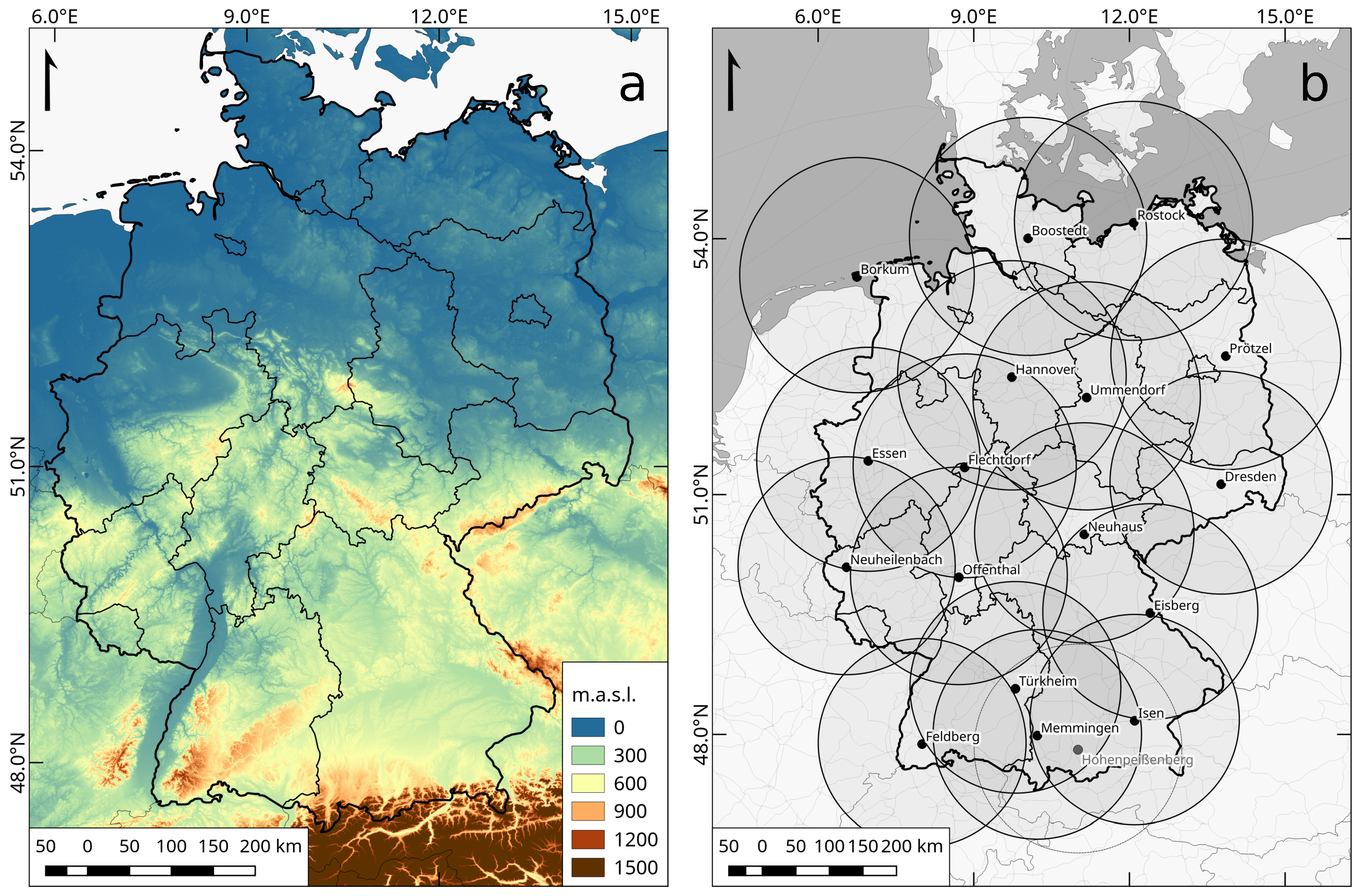
2. Study Area
3. Data and Methodology
3.1. Datasets
3.1.1. Weather Radar Data
3.1.2. Satellite Data
3.1.3. Preprocessing of Datasets
3.2. Methodology
4. Results
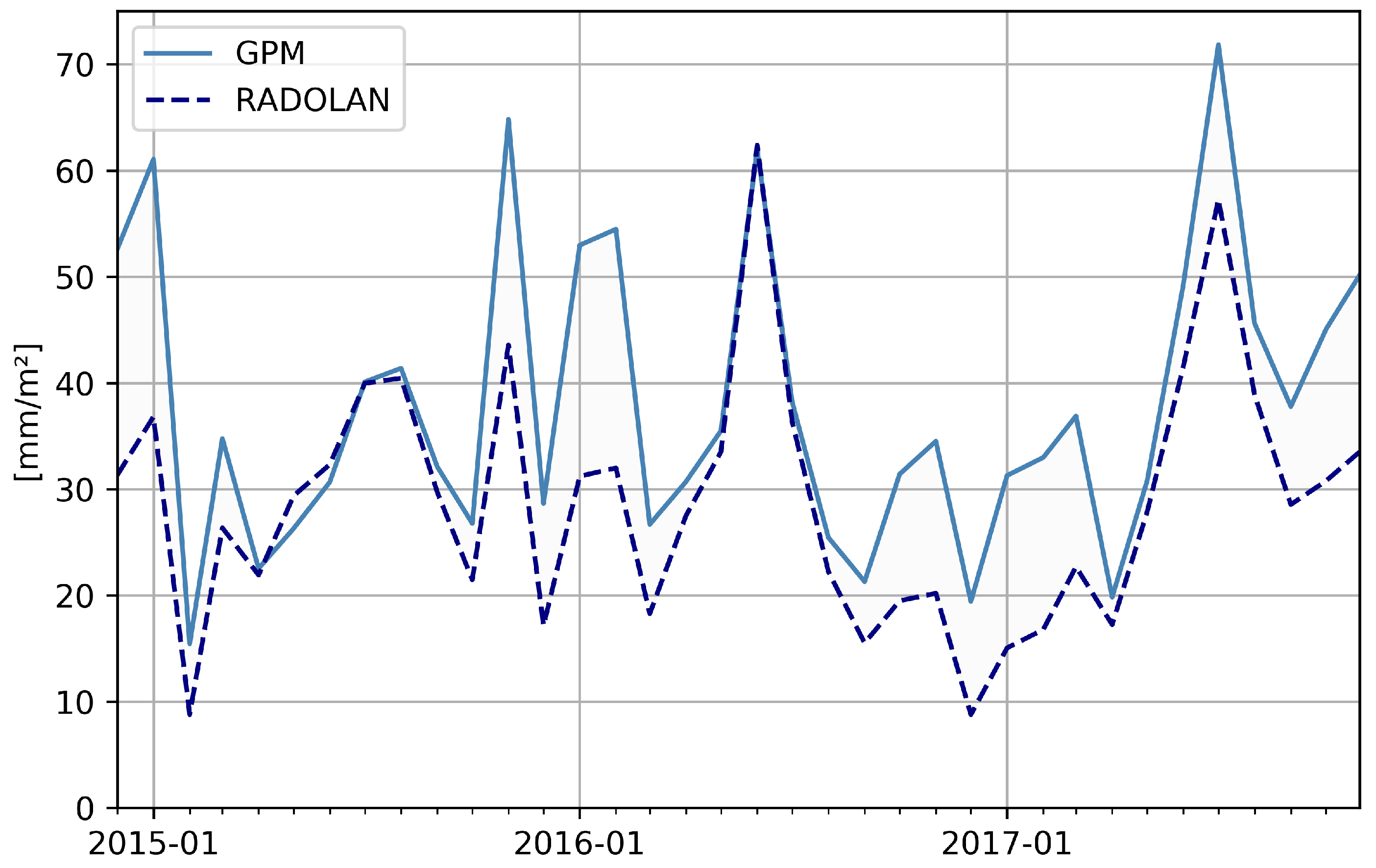
4.1. Statistical Analysis
4.1.1. Overall
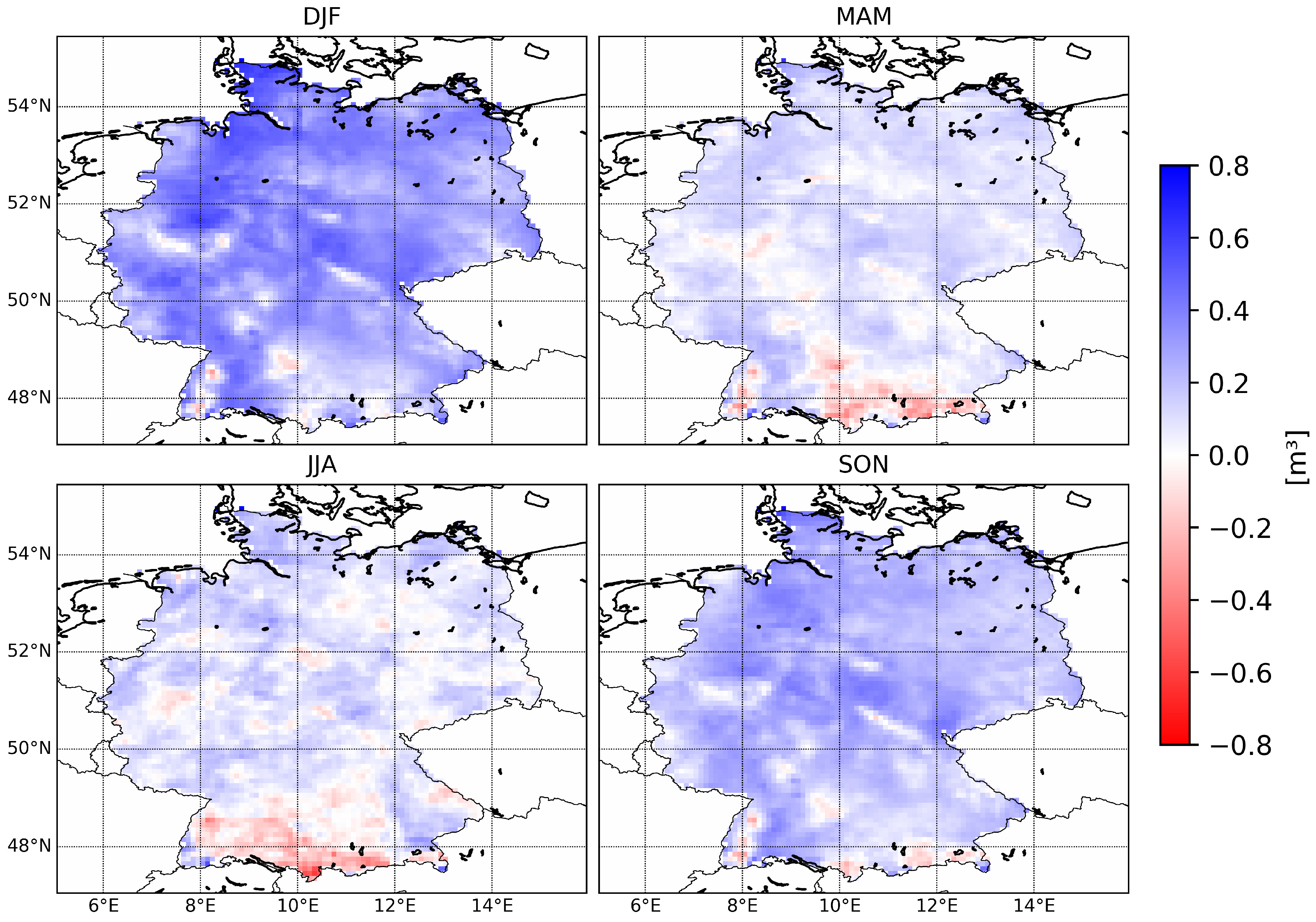
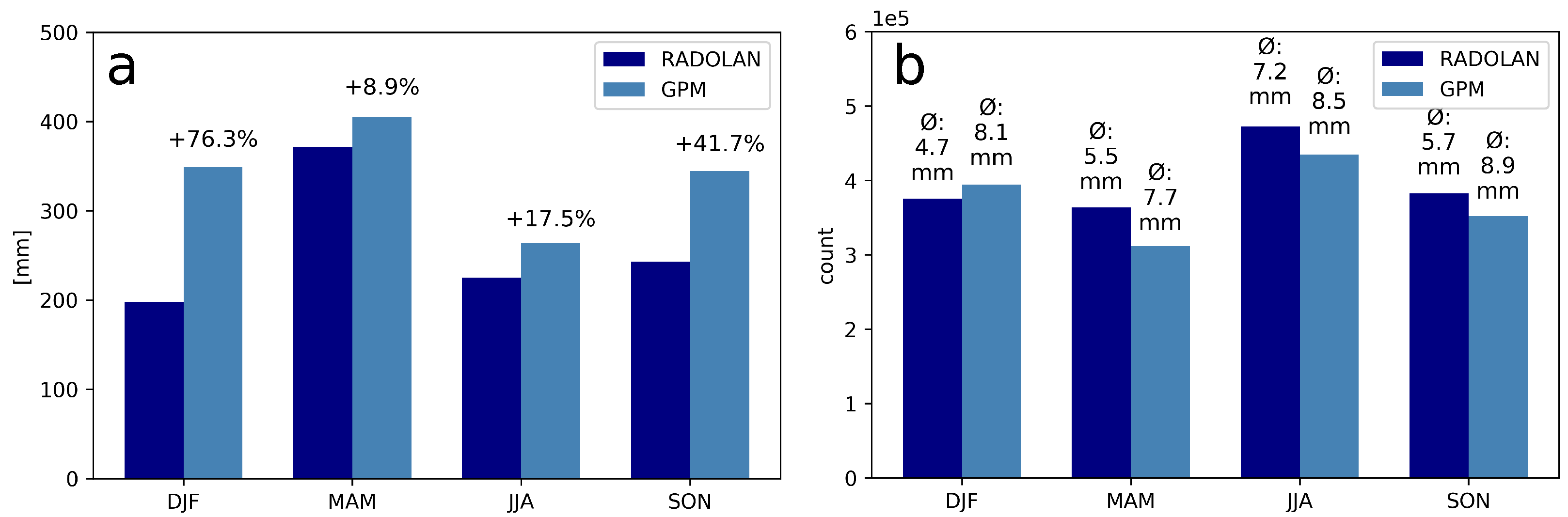
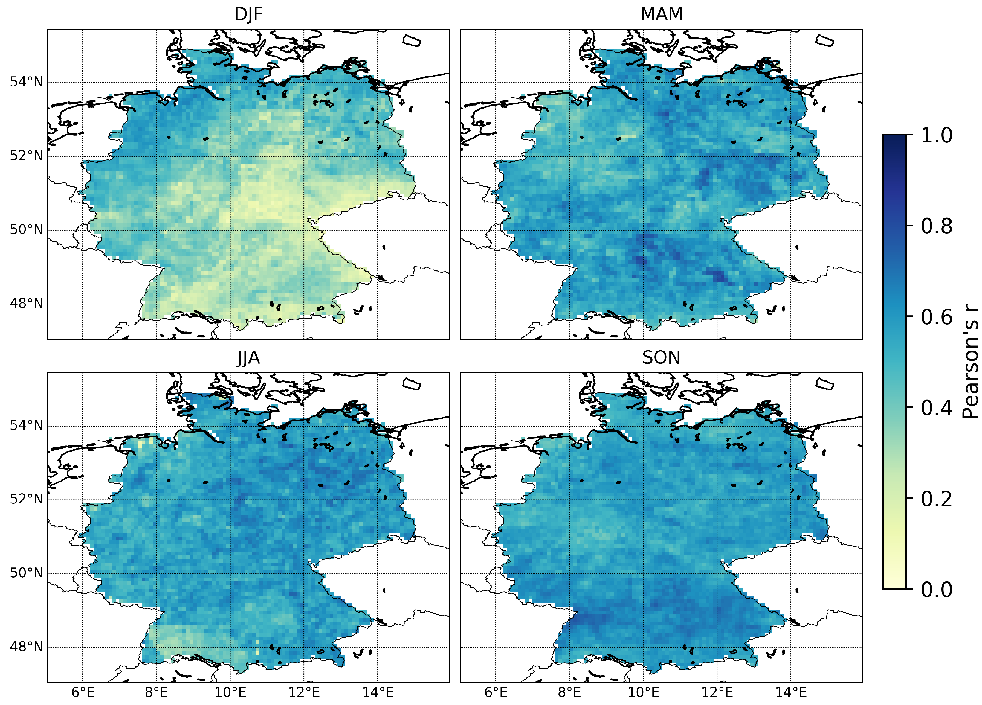
4.1.2. Seasonal Analysis
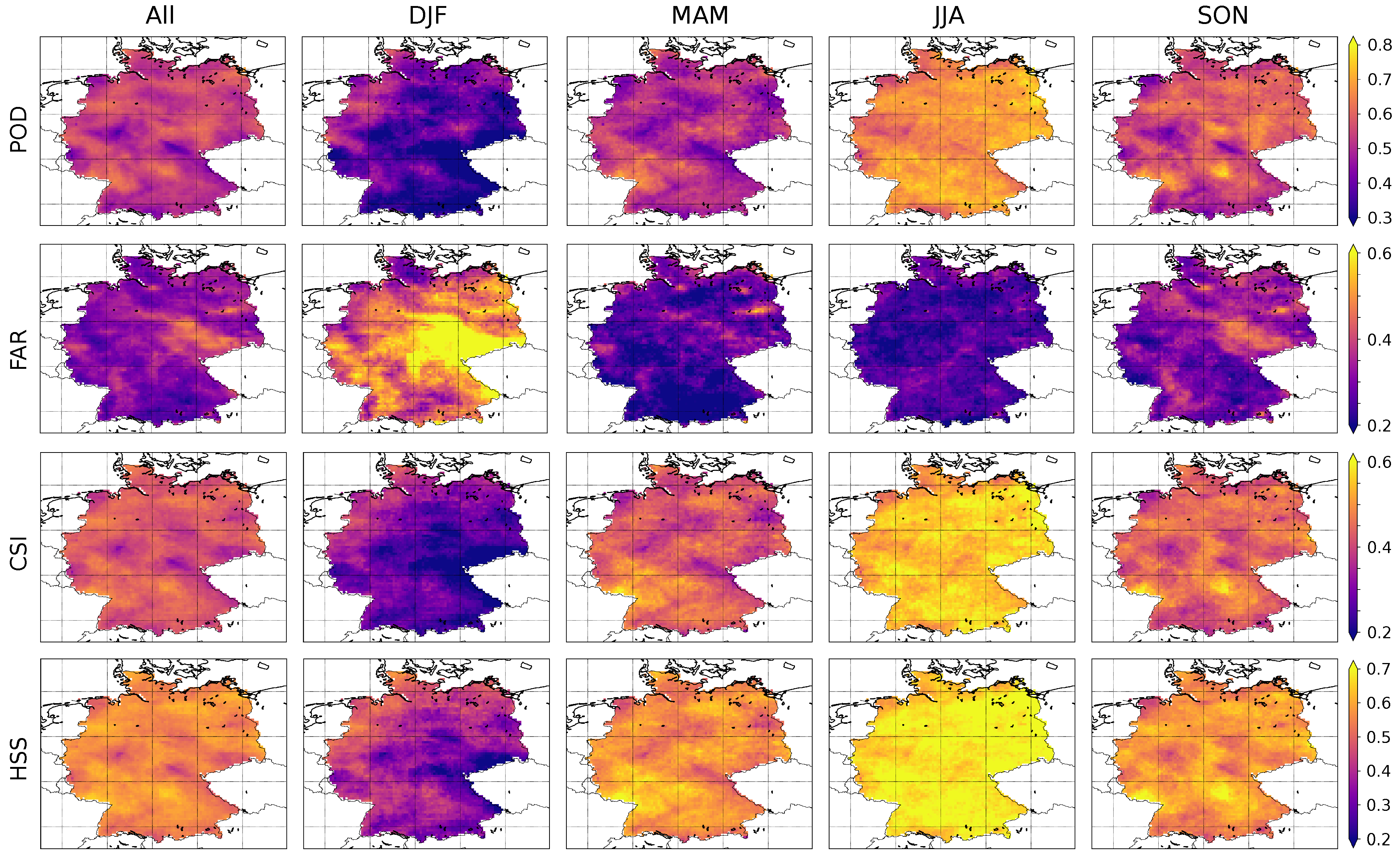
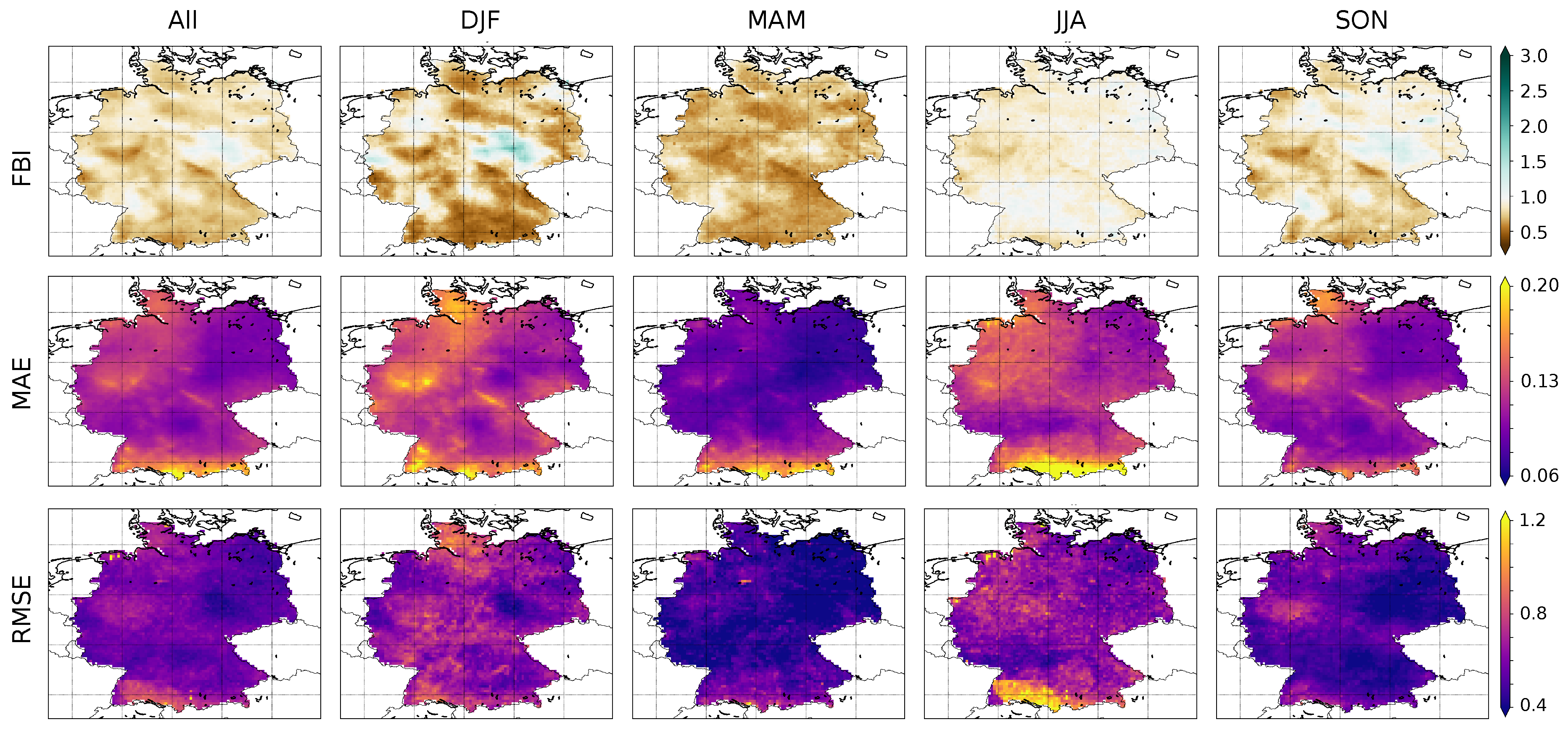
4.2. Categorical Performance
5. Discussion
6. Conclusions
Author Contributions
Funding
Acknowledgments
Conflicts of Interest
References
- GCOS. The Global Observing System for Climate: Implementation Needs; WMO Pub GCOS-200; GCOS: Geneva, Switzerland, 2016. [Google Scholar]
- Kidd, C.; Becker, A.; Huffman, G.J.; Muller, C.L.; Joe, P.; Skofronick-Jackson, G.; Kirschbaum, D.B. So, How Much of the Earth’s Surface Is Covered by Rain Gauges? Bull. Am. Meteorol. Soc. 2017, 98, 69–78. [Google Scholar] [CrossRef]
- Tarpanelli, A.; Massari, C.; Ciabatta, L.; Filippucci, P.; Amarnath, G.; Brocca, L. Exploiting a constellation of satellite soil moisture sensors for accurate rainfall estimation. Adv. Water Resour. 2017, 108, 249–255. [Google Scholar] [CrossRef]
- Román-Cascón, C.; Pellarin, T.; Gibon, F.; Brocca, L.; Cosme, E.; Crow, W.; Fernández-Prieto, D.; Kerr, Y.H.; Massari, C. Correcting satellite-based precipitation products through SMOS soil moisture data assimilation in two land-surface models of different complexity: API and SURFEX. Remote Sens. Environ. 2017, 200, 295–310. [Google Scholar] [CrossRef]
- Crow, W.; van Den Berg, M.; Huffman, G.; Pellarin, T. Correcting rainfall using satellite-based surface soil moisture retrievals: The Soil Moisture Analysis Rainfall Tool (SMART). Water Resour. Res. 2011, 47. [Google Scholar] [CrossRef]
- Ciabatta, L.; Brocca, L.; Massari, C.; Moramarco, T.; Puca, S.; Rinollo, A.; Gabellani, S.; Wagner, W. Integration of Satellite Soil Moisture and Rainfall Observations over the Italian Territory. J. Hydrometeorol. 2015, 16, 1341–1355. [Google Scholar] [CrossRef]
- Brocca, L.; Moramarco, T.; Melone, F.; Wagner, W. A new method for rainfall estimation through soil moisture observations. Geophys. Res. Lett. 2013, 40, 853–858. [Google Scholar] [CrossRef]
- Crow, W.T.; Huffman, G.J.; Bindlish, R.; Jackson, T.J. Improving Satellite-Based Rainfall Accumulation Estimates Using Spaceborne Surface Soil Moisture Retrievals. J. Hydrometeorol. 2009, 10, 199–212. [Google Scholar] [CrossRef]
- Beck, H.E.; Vergopolan, N.; Pan, M.; Levizzani, V.; van Dijk, A.I.J.M.; Weedon, G.; Brocca, L.; Pappenberger, F.; Huffman, G.J.; Wood, E.F. Global-scale evaluation of 23 precipitation datasets using gauge observations and hydrological modeling. Hydrol. Earth Syst. Sci. Discuss. 2017, 2017, 1–23. [Google Scholar] [CrossRef]
- Simpson, J.; Adler, R.F.; North, G.R. A proposed tropical rainfall measuring mission (TRMM) satellite. Bull. Am. Meteorol. Soc. 1988, 69, 278–295. [Google Scholar] [CrossRef]
- Skofronick-Jackson, G.; Petersen, W.A.; Berg, W.; Kidd, C.; Stocker, E.F.; Kirschbaum, D.B.; Kakar, R.; Braun, S.A.; Huffman, G.J.; Iguchi, T.; et al. The Global Precipitation Measurement (GPM) Mission for Science and Society. Bull. Am. Meteorol. Soc. 2017, 98, 1679–1695. [Google Scholar] [CrossRef]
- Huffman, G.J.; Bolvin, D.T.; Braithwaite, D.; Hsu, K.; Joyce, R.; Kidd, C.; Nelkin, E.J.; Sorooshian, S.; Tan, J.; Xie, P. NASA Global Precipitation Measurement (GPM) Integrated Multi-satellitE Retrievals for GPM (IMERG) Algorithm Theoretical and Basis Document and (ATBD) and Version 5.2; Technical Report; National Aeronautics and Space Administration: Greenbelt, MD, USA, 2018.
- Hou, A.Y.; Kakar, R.K.; Neeck, S.; Azarbarzin, A.A.; Kummerow, C.D.; Kojima, M.; Oki, R.; Nakamura, K.; Iguchi, T. The Global Precipitation Measurement Mission. Bull. Am. Meteorol. Soc. 2014, 95, 701–722. [Google Scholar] [CrossRef]
- Liu, Z. Comparison of Integrated Multisatellite Retrievals for GPM (IMERG) and TRMM Multisatellite Precipitation Analysis (TMPA) Monthly Precipitation Products: Initial Results. J. Hydrometeorol. 2016, 17, 777–790. [Google Scholar] [CrossRef]
- Boluwade, A.; Stadnyk, T.; Fortin, V.; Roy, G. Assimilation of precipitation Estimates from the Integrated Multisatellite Retrievals for GPM (IMERG, early Run) in the Canadian Precipitation Analysis (CaPA). J. Hydrol. Reg. Stud. 2017, 14, 10–22. [Google Scholar] [CrossRef]
- Tan, M.; Duan, Z. Assessment of GPM and TRMM Precipitation Products over Singapore. Remote Sens. 2017, 9, 720. [Google Scholar] [CrossRef]
- Tan, M.L.; Santo, H. Comparison of GPM IMERG, TMPA 3B42 and PERSIANN-CDR satellite precipitation products over Malaysia. Atmos. Res. 2018, 202, 63–76. [Google Scholar] [CrossRef]
- He, Z.; Yang, L.; Tian, F.; Ni, G.; Hou, A.; Lu, H. Intercomparisons of Rainfall Estimates from TRMM and GPM Multisatellite Products over the Upper Mekong River Basin. J. Hydrometeorol. 2017, 18, 413–430. [Google Scholar] [CrossRef]
- Tang, G.; Ma, Y.; Long, D.; Zhong, L.; Hong, Y. Evaluation of GPM Day-1 IMERG and TMPA Version-7 legacy products over Mainland China at multiple spatiotemporal scales. J. Hydrol. 2016, 533, 152–167. [Google Scholar] [CrossRef]
- Zhao, H.; Yang, B.; Yang, S.; Huang, Y.; Dong, G.; Bai, J.; Wang, Z. Systematical estimation of GPM-based global satellite mapping of precipitation products over China. Atmos. Res. 2018, 201, 206–217. [Google Scholar] [CrossRef]
- Prakash, S.; Mitra, A.K.; AghaKouchak, A.; Liu, Z.; Norouzi, H.; Pai, D. A preliminary assessment of GPM-based multi-satellite precipitation estimates over a monsoon dominated region. J. Hydrol. 2018, 556, 865–876. [Google Scholar] [CrossRef]
- Sharifi, E.; Steinacker, R.; Saghafian, B. Assessment of GPM-IMERG and Other Precipitation Products against Gauge Data under Different Topographic and Climatic Conditions in Iran: Preliminary Results. Remote Sens. 2016, 8, 135. [Google Scholar] [CrossRef]
- Mahmoud, M.T.; Al-Zahrani, M.A.; Sharif, H.O. Assessment of global precipitation measurement satellite products over Saudi Arabia. J. Hydrol. 2018, 559, 1–12. [Google Scholar] [CrossRef]
- Nikolopoulos, E.I.; Anagnostou, E.N.; Hossain, F.; Gebremichael, M.; Borga, M. Understanding the Scale Relationships of Uncertainty Propagation of Satellite Rainfall through a Distributed Hydrologic Model. J. Hydrometeorol. 2010, 11, 520–532. [Google Scholar] [CrossRef]
- Li, Y.; Grimaldi, S.; Walker, J.; Pauwels, V. Application of Remote Sensing Data to Constrain Operational Rainfall-Driven Flood Forecasting: A Review. Remote Sens. 2016, 8, 456. [Google Scholar] [CrossRef]
- Maggioni, V.; Massari, C. On the performance of satellite precipitation products in riverine flood modeling: A review. J. Hydrol. 2018, 558, 214–224. [Google Scholar] [CrossRef]
- Mei, Y.; Anagnostou, E.N.; Shen, X.; Nikolopoulos, E.I. Decomposing the satellite precipitation error propagation through the rainfall-runoff processes. Adv. Water Resour. 2017, 109, 253–266. [Google Scholar] [CrossRef]
- Rossi, M.; Luciani, S.; Valigi, D.; Kirschbaum, D.; Brunetti, M.; Peruccacci, S.; Guzzetti, F. Statistical approaches for the definition of landslide rainfall thresholds and their uncertainty using rain gauge and satellite data. Geomorphology 2017, 285, 16–27. [Google Scholar] [CrossRef]
- Marra, F.; Destro, E.; Nikolopoulos, E.I.; Zoccatelli, D.; Creutin, J.D.; Guzzetti, F.; Borga, M. Impact of rainfall spatial aggregation on the identification of debris flow occurrence thresholds. Hydrol. Earth Syst. Sci. 2017, 21, 4525–4532. [Google Scholar] [CrossRef]
- Mei, Y.; Nikolopoulos, E.; Anagnostou, E.; Zoccatelli, D.; Borga, M. Error Analysis of Satellite Precipitation-Driven Modeling of Flood Events in Complex Alpine Terrain. Remote Sens. 2016, 8, 293. [Google Scholar] [CrossRef]
- Kugler, Z.; De Groeve, T. The Global Flood Detection System; JRC Scientific and Technical Reports; European Communities: Luxembourg, 2007; pp. 1–45. [Google Scholar]
- Revilla-Romero, B.; Wanders, N.; Burek, P.; Salamon, P.; de Roo, A. Integrating remotely sensed surface water extent into continental scale hydrology. J. Hydrol. 2016, 543, 659–670. [Google Scholar] [CrossRef]
- Revilla-Romero, B.; Thielen, J.; Salamon, P.; Groeve, T.D.; Brakenridge, G.R. Evaluation of the satellite-based Global Flood Detection System for measuring river discharge: influence of local factors. Hydrol. Earth Syst. Sci. 2014, 18, 4467–4484. [Google Scholar] [CrossRef]
- Speirs, P.; Gabella, M.; Berne, A. A Comparison between the GPM Dual-Frequency Precipitation Radar and Ground-Based Radar Precipitation Rate Estimates in the Swiss Alps and Plateau. J. Hydrometeorol. 2017, 18, 1247–1269. [Google Scholar] [CrossRef]
- Zhang, A.; Chen, S.; Fan, S. Comparison of Extreme Precipitation Estimation From GPM Dual-Frequency Radar and Ground-Based Radar Network in Southern China. In Proceedings of the 2017 IEEE International Geoscience and Remote Sensing Symposium (IGARSS), Fort Worth, TX, USA, 23–28 July 2017; pp. 4534–4537. [Google Scholar]
- Gabella, M.; Speirs, P.; Hamann, U.; Germann, U.; Berne, A. Measurement of Precipitation in the Alps Using Dual-Polarization C-Band Ground-Based Radars, the GPM Spaceborne Ku-Band Radar, and Rain Gauges. Remote Sens. 2017, 9, 1147. [Google Scholar] [CrossRef]
- Cannon, F.; Ralph, F.M.; Wilson, A.M.; Lettenmaier, D.P. GPM Satellite and Radar Measurements and of Precipitation and Freezing Level and in Atmospheric Rivers: Comparison with Ground-Based Radars and Reanalyses. J. Geophys. Res. Atmos. Forest. 2017, 122, 12747–12764. [Google Scholar] [CrossRef]
- Gao, J.; Tang, G.; Hong, Y. Similarities and Improvements of GPM Dual-Frequency Precipitation Radar (DPR) upon TRMM Precipitation Radar (PR) in Global Precipitation Rate Estimation, Type Classification and Vertical Profiling. Remote Sens. 2017, 9, 1142. [Google Scholar] [CrossRef]
- Biswas, S.K.; Le, M.; Chandrasekar, V. Identification of Snow from GPM-DPR observations and cross validation with S-Band Ground Radar dual polarization measurements. In Proceedings of the 32 nd URSI GASS, Montreal, QC, Canada, 19–26 August 2017. [Google Scholar]
- Skofronick-Jackson, G.; Hudak, D.; Petersen, W.; Nesbitt, S.W.; Chandrasekar, V.; Durden, S.; Gleicher, K.J.; Huang, G.J.; Joe, P.; Kollias, P.; et al. Global Precipitation Measurement Cold Season Precipitation Experiment (GCPEX): For Measurement’s Sake, Let It Snow. Bull. Am. Meteorol. Soc. 2015, 96, 1719–1741. [Google Scholar] [CrossRef]
- You, Y.; Wang, N.Y.; Ferraro, R.; Rudlosky, S. Quantifying the Snowfall Detection Performance of the GPM Microwave Imager Channels over Land. J. Hydrometeorol. 2017, 18, 729–751. [Google Scholar] [CrossRef]
- Casella, D.; Panegrossi, G.; Sanò, P.; Marra, A.C.; Dietrich, S.; Johnson, B.T.; Kulie, M.S. Evaluation of the GPM-DPR snowfall detection capability: Comparison with CloudSat-CPR. Atmos. Res. 2017, 197, 64–75. [Google Scholar] [CrossRef]
- Wen, Y.; Behrangi, A.; Lambrigtsen, B.; Kirstetter, P.E. Evaluation and Uncertainty Estimation of the Latest Radar and Satellite Snowfall Products Using SNOTEL Measurements over Mountainous Regions in Western United States. Remote Sens. 2016, 8, 904. [Google Scholar] [CrossRef]
- Sharifi, E.; Steinacker, R.; Saghafian, B. Multi time-scale evaluation of high-resolution satellite-based precipitation products over northeast of Austria. Atmos. Res. 2018, 206, 46–63. [Google Scholar] [CrossRef]
- Rysman, J.F.; Panegrossi, G.; Sanò, P.; Marra, A.; Dietrich, S.; Milani, L.; Kulie, M. SLALOM: An All-Surface Snow Water Path Retrieval Algorithm for the GPM Microwave Imager. Remote Sens. 2018, 10, 1278. [Google Scholar] [CrossRef]
- Gampe, D.; Ludwig, R. Evaluation of Gridded Precipitation Data Products for Hydrological Applications in Complex Topography. Hydrology 2017, 4, 53. [Google Scholar] [CrossRef]
- RADOLAN/RADVOR Hoch aufgelöste Niederschlagsanalyse und –Vorhersage auf der Basis Quantitativer Radar und Ombrometerdaten für and grenzüberschreitende Fluss-Einzugsgebiete von Deutschland im Echtzeitbetrieb Beschreibung des Kompositformats Version 2.4.3; Technical Report; Deutscher Wetterdienst, Abteilung Hydrometeorologie: Offenbach, Germany, 2018.
- Bartels, H. Projekt RADOLAN. Routineverfahren zur Online-Aneichung der Radarniederschlagsdaten mit Hilfe von Automatischen Bodenniederschlagsstationen (Ombrometer); Technical Report; Deutscher Wetterdienst, Hydrometeorologie: Offenbach, Germany, 2004.
- Meyer, H.; Kühnlein, M.; Appelhans, T.; Nauss, T. Comparison of Four Machine Learning Algorithms for Their Applicability in Satellite-Based Optical Rainfall Retrievals. Atmos. Res. 2016, 169, 424–433. [Google Scholar] [CrossRef]
- Kühnlein, M.; Appelhans, T.; Thies, B.; Nauss, T. Improving the accuracy of rainfall rates from optical satellite sensors with machine learning—A random forests-based approach applied to MSG SEVIRI. Remote Sens. Environ. 2014, 141, 129–143. [Google Scholar] [CrossRef]
- Bronstert, A.; Agarwal, A.; Boessenkool, B.; Crisologo, I.; Fischer, M.; Heistermann, M.; Köhn-Reich, L.; López-Tarazón, J.A.; Moran, T.; Ozturk, U.; et al. Forensic hydro-meteorological analysis of an extreme flash flood: The 2016-05-29 event in Braunsbach, SW Germany. Sci. Total Environ. 2018, 630, 977–991. [Google Scholar] [CrossRef]
- Doycheva, K.; Horn, G.; Koch, C.; Schumann, A.; König, M. Assessment and weighting of meteorological ensemble forecast members based on supervised machine learning with application to runoff simulations and flood warning. Adv. Eng. Inform. 2017, 33, 427–439. [Google Scholar] [CrossRef]
- Fischer, F.; Hauck, J.; Brandhuber, R.; Weigl, E.; Maier, H.; Auerswald, K. Spatio-temporal variability of erosivity estimated from highly resolved and adjusted radar rain data (RADOLAN). Agric. For. Meteorol. 2016, 223, 72–80. [Google Scholar] [CrossRef]
- Winterrath, T.; Brendel, C.; Hafer, M.; Junghänel, T.; Klameth, A.; Walawender, E.; und Andreas Becker, E.W. Erstellung Einer Radargestützten Niederschlagsklimatologie; Berichte des Deutschen Wetterdienstes; Deutschen Wetterdienstes: Offenbach am Main, Germany, 2017; Volume 251, pp. 1–71.
- Winterrath, T.; Rosenow, W.; Weigl, E. On the DWD quantitative precipitation analysis and nowcasting system for real-time application in German flood risk management. Weather Radar Hydrol. 2012, 351, 323–329. [Google Scholar]
- Keupp, L.; Winterrath, T.; Hollmann, R. Use of Weather Radar Data for Climate Data Records in WMO Regions IV and VI; Technical Report, WMO CCl TT-URSDCM; WMO: Geneva, Switzerland, 2017. [Google Scholar]
- Richter, D. Ergebnisse methodischer Untersuchungen zur Korrektur des Systematischen Meßfehlers des Hellmann-Niederschlagmessers. Deutschen Wetterdienstes: Offenbach am Main, Germany, 1995; Volume 194, pp. 1–93. [Google Scholar]
- World Meteorological Organization. Guide to Meteorological Instruments and Methods of Observation, WMO-No. 8; World Meteorological Organization: Geneva, Switzerland, 2017. [Google Scholar]
- Becker, A.; Finger, P.; Meyer-Christoffer, A.; Rudolf, B.; Schamm, K.; Schneider, U.; Ziese, M. A description of the global land-surface precipitation data products of the Global Precipitation Climatology Centre with sample applications including centennial (trend) analysis from 1901–present. Earth Syst. Sci. Data 2013, 5, 71–99. [Google Scholar] [CrossRef]
- Ullrich, P.A.; Taylor, M.A. Arbitrary-Order Conservative and Consistent Remapping and a Theory of Linear Maps: Part I. Mon. Weather Rev. 2015, 143, 2419–2440. [Google Scholar] [CrossRef]
- Chen, C.T.; Knutson, T. On the Verification and Comparison of Extreme Rainfall Indices from Climate Models. J. Clim. 2008, 21, 1605–1621. [Google Scholar] [CrossRef]
- Accadia, C.; Mariani, S.; Casaioli, M.; Lavagnini, A.; Speranza, A. Sensitivity of precipitation forecast skill scores to bilinear interpolation and a simple nearest-neighbor average method on high-resolution verification grids. Weather Forecast. 2003, 18, 918–932. [Google Scholar] [CrossRef]
- Chen, C.J.; Senarath, S.U.S.; Dima-West, I.M.; Marcella, M.P. Evaluation and restructuring of gridded precipitation data over the Greater Mekong Subregion. Int. J. Climatol. 2016, 37, 180–196. [Google Scholar] [CrossRef]
- Jones, P.W. First- and Second-Order Conservative Remapping Schemes for Grids in Spherical Coordinates. Mon. Weather Rev. 1999, 127, 2204–2210. [Google Scholar] [CrossRef]
- Jones, P.W. A User’s Guide for SCRIP: A Spherical Coordinate Remapping and Interpolation Package, Version 1.5; Los Alamos National Laboratory: Los Alamos, NM, USA, 1998.
- Schulzweida, U. CDO User Guide; Technical Report; MPI for Meteorology: Hamburg, Germany, 2018. [Google Scholar]
- Kalognomou, E.A.; Lennard, C.; Shongwe, M.; Pinto, I.; Favre, A.; Kent, M.; Hewitson, B.; Dosio, A.; Nikulin, G.; Panitz, H.J.; et al. A Diagnostic Evaluation of Precipitation in CORDEX Models over Southern Africa. J. Clim. 2013, 26, 9477–9506. [Google Scholar] [CrossRef]
- Diaconescu, E.P.; Gachon, P.; Laprise, R. On the Remapping Procedure of Daily Precipitation Statistics and Indices Used in Regional Climate Model Evaluation. J. Hydrometeorol. 2015, 16, 2301–2310. [Google Scholar] [CrossRef]
- Wang, J.; Zeng, N.; Wang, M.; Jiang, F.; Chen, J.; Friedlingstein, P.; Jain, A.K.; Jiang, Z.; Ju, W.; Lienert, S.; et al. Contrasting interannual atmospheric CO2 variabilities and their terrestrial mechanisms for two types of El Niños. Atmos. Chem. Phys. 2018, 18, 10333–10345. [Google Scholar] [CrossRef]
- Woodcock, F. The evaluation of yes/no forecasts for scientific and administrative purposes. Mon. Weather Rev. 1976, 104, 1209–1214. [Google Scholar] [CrossRef]
- Doswell, C.A.; Davies-Jones, R.; Keller, D.L. On summary measures of skill in rare event forecasting based on contingency tables. Weather Forecast. 1990, 5, 576–585. [Google Scholar] [CrossRef]
- Schaefer, J.T. The critical success index as an indicator of warning skill. Weather Forecast. 1990, 5, 570–575. [Google Scholar] [CrossRef]
- Kochendorfer, J.; Rasmussen, R.; Wolff, M.; Baker, B.; Hall, M.E.; Meyers, T.; Landolt, S.; Jachcik, A.; Isaksen, K.; Brækkan, R.; et al. The quantification and correction of wind-induced precipitation measurement errors. Hydrol. Earth Syst. Sci. 2017, 21, 1973–1989. [Google Scholar] [CrossRef]
- Boudala, F.S.; Isaac, G.A.; Filman, P.; Crawford, R.; Hudak, D.; Anderson, M. Performance of Emerging Technologies for Measuring Solid and Liquid Precipitation in Cold Climate as Compared to the Traditional Manual Gauges. J. Atmos. Ocean. Technol. 2017, 34, 167–185. [Google Scholar] [CrossRef]


| RADOLAN | |||
|---|---|---|---|
| Rain | No Rain | ||
| GPM | rain | a | b |
| no rain | c | d | |
| Season | All | DJF | MAM | JJA | SON |
|---|---|---|---|---|---|
| Probability Of Detection (POD) | 0.53 | 0.38 | 0.51 | 0.67 | 0.56 |
| False Alarm Ratio (FAR) | 0.32 | 0.48 | 0.25 | 0.25 | 0.32 |
| Critical Success Index (CSI) | 0.42 | 0.28 | 0.43 | 0.55 | 0.44 |
| Heidke Skill Score (HSS) | 0.56 | 0.39 | 0.57 | 0.68 | 0.58 |
| Frequency Bias Index (FBI) | 0.78 | 0.72 | 0.68 | 0.90 | 0.83 |
| Mean Absolute Error (MAE) | 0.11 | 0.12 | 0.08 | 0.12 | 0.10 |
| Root Mean Square Error (RMSE) | 0.59 | 0.66 | 0.47 | 0.67 | 0.52 |
© 2018 by the authors. Licensee MDPI, Basel, Switzerland. This article is an open access article distributed under the terms and conditions of the Creative Commons Attribution (CC BY) license (http://creativecommons.org/licenses/by/4.0/).
Share and Cite
Ramsauer, T.; Weiß, T.; Marzahn, P. Comparison of the GPM IMERG Final Precipitation Product to RADOLAN Weather Radar Data over the Topographically and Climatically Diverse Germany. Remote Sens. 2018, 10, 2029. https://doi.org/10.3390/rs10122029
Ramsauer T, Weiß T, Marzahn P. Comparison of the GPM IMERG Final Precipitation Product to RADOLAN Weather Radar Data over the Topographically and Climatically Diverse Germany. Remote Sensing. 2018; 10(12):2029. https://doi.org/10.3390/rs10122029
Chicago/Turabian StyleRamsauer, Thomas, Thomas Weiß, and Philip Marzahn. 2018. "Comparison of the GPM IMERG Final Precipitation Product to RADOLAN Weather Radar Data over the Topographically and Climatically Diverse Germany" Remote Sensing 10, no. 12: 2029. https://doi.org/10.3390/rs10122029
APA StyleRamsauer, T., Weiß, T., & Marzahn, P. (2018). Comparison of the GPM IMERG Final Precipitation Product to RADOLAN Weather Radar Data over the Topographically and Climatically Diverse Germany. Remote Sensing, 10(12), 2029. https://doi.org/10.3390/rs10122029