Abstract
Monitoring the development of vegetation height through time provides a key indicator of crop health and overall condition. Traditional manual approaches for monitoring crop height are generally time consuming, labor intensive and impractical for large-scale operations. Dynamic crop heights collected through the season allow for the identification of within-field problems at critical stages of the growth cycle, providing a mechanism for remedial action to be taken against end of season yield losses. With advances in unmanned aerial vehicle (UAV) technologies, routine monitoring of height is now feasible at any time throughout the growth cycle. To demonstrate this capability, five digital surface maps (DSM) were reconstructed from high-resolution RGB imagery collected over a field of maize during the course of a single growing season. The UAV retrievals were compared against LiDAR scans for the purpose of evaluating the derived point clouds capacity to capture ground surface variability and spatially variable crop height. A strong correlation was observed between structure-from-motion (SfM) derived heights and pixel-to-pixel comparison against LiDAR scan data for the intra-season bare-ground surface (R2 = 0.77 − 0.99, rRMSE = 0.44% − 0.85%), while there was reasonable agreement between canopy comparisons (R2 = 0.57 − 0.65, rRMSE = 37% − 50%). To examine the effect of resolution on retrieval accuracy and processing time, an evaluation of several ground sampling distances (GSD) was also performed. Our results indicate that a 10 cm resolution retrieval delivers a reliable product that provides a compromise between computational cost and spatial fidelity. Overall, UAV retrievals were able to accurately reproduce the observed spatial variability of crop heights within the maize field through the growing season and provide a valuable source of information with which to inform precision agricultural management in an operational context.
1. Introduction
Over the last decade, there has been a surge of interest in the development and use of unmanned aerial vehicles (UAVs) for agricultural and environmental applications [1,2,3]. The opportunities presented by these emergent earth observation systems have revolutionized the manner in which spatial information can be retrieved, offering new capacity for on-demand sensing and high spatio-temporal coverage [4]. UAVs have the capacity to provide remotely sensed data in real time and in the field and do not suffer from the inherent lag of satellite and aircraft-based imagery [3]. It is this increased speed of image interpretation, together with the associated spatial and temporal improvements, that show potential for changing how farmers interact with and respond to their fields. Overall, advances in UAV platforms [5], sensors design and miniaturization [6], improvements in imaging techniques and processing workflows [7], as well as the availability of ultra-high temporal and spatial resolution data [4] are revolutionizing the way in which environmental monitoring applications can be undertaken [8].
One area where UAVs have shown considerable potential is through their application in precision agriculture. Precision agriculture involves the use of geospatial techniques and sensors to identify variations within the field, with a purpose of aiding crop production via targeted use of inputs and leading to reduced yield losses from nutrient imbalance, weed outbreaks or insect damage [9]. In line with this, a range of remote sensing system has been applied to investigate aspects such as crop fraction [10], weed detection [11,12] and vegetation properties via both hyperspectral [13,14] and multispectral [15] sensors. Thermal and LiDAR sensor have also been deployed to estimate evaporative fluxes [16] as well as crop height monitoring [17,18], respectively.
Measuring canopy phenotypic variables such as crop height is of much interest to researchers and agronomists, since it can be used to determine crop management strategies for maximizing crop yield. Indeed, crop height is one of the most direct indicators of plant growth and development and can be indirectly related to productivity and growth rate [19,20]. For instance, under normal conditions, plants are expected to grow to a certain height during each growth state [21]. In contrast, if a plant is stressed due to disease or a lack of water or nutrients, its growth rate may be negatively affected, potentially reducing the final crop yield [22,23]. Several previous studies focusing on crop height estimation have highlighted its importance as a key indicator for monitoring health and condition. For instance, crop height has been positively correlated with the crop yield [24,25,26] and exhibits a close relationship with crop biomass [27,28] and soil nitrogen supply [29].
As plant breeders strive to develop better hybrids to meet current and future food demand, repeated phenotypic measurements of canopy properties over large fields are often required [30]. Commonly used manual approaches for monitoring crop height are time consuming, labor intensive and impractical for large-scale commercial operations. Furthermore, they do not generally provide the intra- or inter-field spatial variability, which is a key requirement of any precision agricultural based approach. One of the main advantages of UAV-based crop height and growth estimation is that retrievals can be obtained with relatively standard instrumentation, as compared to many other types of remote sensing systems [31,32]. With advances in UAV technologies, routine monitoring of height is now feasible at any time of the growth cycle, providing spatially explicit retrievals on an as-needed or taskable basis [4]. This represents a valuable information resource not only in terms of crop production but also for more general agricultural management, facilitating the detection of intra-field spatial variability that may result from ineffective irrigation practices, fertilizer variability, as well as salinity and other soil property issue. Through such knowledge, the concept of more “crop-per-drop” can be better realized, as too the reduction of unnecessary fertilizer and pesticide application. In dryland environments like Saudi Arabia [33], this concept is even more crucial, as the proportion of water use in agricultural production has been estimated at more than 80% [34], much of which is derived from already over-stressed groundwater systems [35]. It is clear that efforts to enhance food production in such-regions need to consider parallel responses in terms of sustainability and effective management of agricultural systems [36].
The collection of overlapping UAV imagery allows for the reconstruction of the Digital Surface Map (DSM) through application of Structure from Motion (SfM) algorithms [37,38], a photogrammetric imaging technique used to estimate three-dimensional structures from two-dimensional image sequence. To do this, large collections of RGB imagery derived from miniaturized sensors onboard UAVs can be automatically processed for aerial triangulation and camera orientation adjustments. The image overlap is then exploited by computer vision algorithms to find correspondence between images and features such as corner points (edges with gradients in multiple directions), which are tracked from one image to the next. Over the course of the last decade, a number of commercial and open-source software has been developed with the aim of providing users with accurate DSMs [39]. In combination with appropriate georeferencing, these data provide a capacity to extract and assess crop height and growth [40,41]. Nevertheless, estimating the absolute crop height above ground from a DSM remains problematic because of a lack of knowledge on the elevation and variability of the underlying terrain. Although different methodologies have been proposed to extract crop height from a DSM, retrieving a bare soil map (without vegetation on the surface) that is subsequently subtracted from a DSM, remains the most convenient method to retrieve crop height. A number of previous studies have demonstrated the efficiency of the “difference method” in delivering reliable crop height values [42,43]. When compared to methodologies that use landcover separation techniques to discriminate between terrain (soil) and vegetation (hence enabling crop height to be determined from a single flight without the need of a bare soil map) [31,32,44,45], the difference approach has proven to be simpler, faster and requires significantly less expertise to produce useful results [46]. The required terrain model (bare soil) for the difference method can be most easily derived by performing a UAV survey immediately before and/or after the sowing date [46].
A number of UAV-based SfM studies have focused on a single UAV campaign to monitor crop height. Such studies examined a variety of agricultural crops, including maize [47], sorghum [47,48], alfalfa [49], vineyards [50,51], sugarcane [52] and olive tree plantations [53]. Despite positive results, a single crop height extraction during the growing season is generally not able to provide the information needed to inform precision agricultural management. Further progress in crop height analyses have assessed the retrieval of multi-temporal crop height using LiDAR [44,54], near-infrared [55] and RGB stereo images captured by UAVs. Among the latter, multi-temporal crop height estimation has been undertaken for maize [32], sorghum [31,32], wheat [46,56] and barley [42,57]. Holman et al. [58] assessed the crop height retrieval of wheat with different nitrogen conditions, while others have examined the relationship between multi-temporal crop height and biomass for forage monitor in grassland [59] and for maize under different levels of nitrogen applications [45]. Bendig et al. [60] estimated barley biomass using dynamic crop height data retrieved from a UAV, while Schirrman et al. [61] evaluated the relationship among multiple biophysical parameters in wheat (i.e., multi-temporal crop height, LAI, nitrogen status and biomass). More recently, Moeckel et al. [62] used the UAV-SfM approach to monitor vegetable crops (i.e., eggplants, tomatoes and cabbage). Despite the successful application of RGB imagery in UAV-based SfM approaches, all of the cited multi-temporal studies have used rotary UAVs, which have tended to limit the crop monitoring to relatively small field scales (i.e., they did not exceed 11 ha [61]). Ultimately, the physical constraints that characterize this type of sensing systems (i.e., lower flight time, flying height and air-speed) enable crop monitoring only at smaller scales.
One of the aims of this contribution was to assess the retrieval of multi-temporal crop height from a fixed-wing UAV over a large commercial scale (50 ha) agricultural field and to examine the practical implementation of this procedure. An extensive evaluation of the intra-field crop variability throughout the growing season is presented and an assessment of the UAV derived crop height is conducted using ground-based LiDAR data via a pixel-by-pixel scale comparison. We determine whether the retrieval of dynamic crop height is applicable at industrial field scales and repeatable over the growth cycle of the crops by conducting five unique surveys and a multi-temporal DSM derived from ultra-high (2.5 cm) resolution RGB imagery. Specific objectives for this study include: (1) evaluating the capacity of a fixed-wing UAV to drive SfM based 3D canopy models at the large field scale, repeatedly and consistently over time; (2) testing and applying a repeatable processing workflow to derive crop height; (3) investigating the accuracy of SfM plant height estimates when compared directly to LiDAR ground measurements; and (4) assessing this comparison at multiple resolution scales (2.5, 5, 10 and 20 cm). Considering the importance of crop height as a metric to assess the health and status of agricultural crops, a further goal of this investigation is to demonstrate its applicability in providing farmers (as well as the research community) with practical guidance for data collection and processing that can be used to inform a typical precision agricultural application.
2. Materials and Methods
2.1. Study Site and Field Conditions
Five UAV campaigns were undertaken over the Tawdeehiya farm (24.174°N, 48.015°E) in the Al Kharj region of Saudi Arabia, approximately 200 km southeast of Riyadh (Figure 1a). 47 fields are operated under center-pivot irrigation, which at the time of the UAV campaigns were planted with a mix of Rhodes grass, alfalfa, maize, carrots and smaller quantities of other vegetables. The study site is characterized as a hot desert climate [63] with a very low annual precipitation of 95 mm that is concentrated between December and April [64]. Records from the farm meteorological station reported that the average daytime maximum temperature during the growing season was 39.4 °C, while the rainfall was limited to 13.5 mm and concentrated in the first two weeks of April. The focus of this investigation is a single 50 ha center-pivot field with a diameter approaching 800 m, planted with maize (Inovi hybrid variety) on 19 March and harvested on 26 June 2016. The cultivar was planted with a row spacing of 50 cm and aiming for a total of 90,000 kernel/ha (which correspond to a plant density of 9 plants/m2). Due to the hot weather conditions and the structure of the soil (mainly sandy soil), the pivot is heavily (and constantly) watered throughout the duration of the growing season. The center-pivot irrigation system has a speed of one revolution every 40 h during the first three weeks of the season and every 60 h for the remaining period (i.e., until harvesting), with the sprinklers delivering 1250 gallons of water per minute.
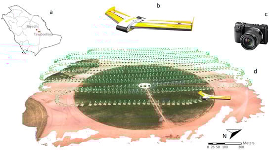
Figure 1.
UAV platform and associated flight path utilized for surveying the maize pivot: (a) location of the Tawdeehiya commercial farm in Saudi Arabia; (b) the Quest UAV and (c) the Sony mirrorless NEX-7 with 24 Mpx sensor deployed onboard of the UAV system; (d) the flight path and camera location of where images were collected.
2.2. Description of UAV Flight Control and Sensor Payload
A remote controlled fixed-wing UAV (QuestUAV, Northumberland, UK) was employed for data collection (Figure 1b). The simple architecture of the UAV (carbon fiber body with single propeller engine and a wingspan of 195 cm) ensures more efficient aerodynamics, providing the advantage of longer flight duration at higher speeds (up to 60 min at an average cruise speed of 35 knots) and enabling a large survey area per given flight. The UAV was deployed with a 24 MP Advanced Photo System type-C compact digital camera (Sony Nex-7) with Complementary Metal-Oxide-Semiconductor sensor (23.5 mm × 15.6 mm) and equipped with a 20 mm wide-angle lens, with max aperture f/2.8 (Figure 1c).
To retrieve the intra-field dynamic crop height of the maize field, multiple UAV flights were conducted over the course of five field campaigns, starting from 15 days after planting and finishing one day before harvesting. The campaigns were conducted under clear sky conditions on Day of Year (DOY) 95, 109, 119, 130 and 177 of the year 2016. In order to ensure consistency amongst the image sequence and to facilitate the DSM reconstruction during post-processing, all flights were planned with a high-frequency shooting time of 1 s and with a high number of flight lines (14 per flight). This ensured an almost 85% frontal overlap and 60% side overlap between each image, which is necessary to identify sufficient key points and to create the 3D point clouds for surface model generation and consistent with the recommended overlap for collected UAV imagery analyzed using SfM [65,66]. It should be noted that due to a camera bay obstruction, the images collected on DOY 109 were partially blocked. To ensure reliable post-processing, the dark portion of each picture was cropped and each EXIF header file updated to include a lower image resolution compared to the other surveys (Table 1).

Table 1.
Summary of captured image dataset, GCPs and GSD.
The UAV was auto-piloted along predefined flight paths created using the UgCS Mapper software (Figure 1d). Flight elevation was set to 120 m above the ground and the flying time ranged between 14 and 15 min, depending on the survey. Based on the aforementioned specifications, a Ground Sampling Distance (GSD) of 2.5 cm (which represents the distance between two consecutive pixel centers measured on the ground) was achieved and subsequently used for the determination of crop height.
In order to correctly place the UAV images in relation to the Earth, several ground control points (GCPs) were used for ensuring an accurate georeferencing of the entire dataset. For this purpose, 15 GCPs were deployed around and within the pivot (Figure 2a) prior to undertaking each UAV flight, with their position measured with an RTK-GPS system (Leica Viva GS10 Base and GS15 Rover, Leica Geosystem, St. Gallen, Switzerland), providing a horizontal and vertical accuracy of 0.8 and 1.5 cm, respectively. The spatial arrangement of the GCPs has been optimized in order to cover the 800 m diameter center pivot and to achieve high crop estimation accuracy over the entire maize field. Previous studies have highlighted the importance of an adequate number and location of GCPs in order to achieve an accurate outcome [67,68]. The GCPs used here were 50 cm × 50 cm plastic frames consisting of a white canvas fabric on which two black triangles were painted from the corners. The configuration provides the vertex in the middle of the frame, from which the GPS measurements were taken (Figure 2c). Table 1 summarizes relevant information on each of the surveys, including the number of images collected, GCPs elevation range and minimum GSD and the geolocation error for each campaign flight.
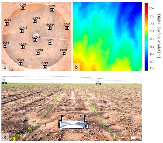
Figure 2.
(a) Spatial arrangement of the 15 ground control points (GCPs) across the maize field (first campaign with recently planted crop shown in this example); and (b) related digital surface model obtained after georeferencing; (c) Ground control point positioning and set up. The GCPs were placed in the field before each UAV flight and their coordinates measured using an RTK-GPS system.
2.3. Image Processing: Georeferencing Using Computer Vision Approaches
Agisoft PhotoScan Professional (Version 1.3) was used to process all the RGB images for each UAV collection, generating the digital surface maps and corresponding orthomosaics. For a reliable DSM reconstruction, consistency of the underlying image data is paramount. As such, prior to initiating the software workflow, a consistent image based specification of a coordinate system was needed. Therefore, we re-projected the WGS 84 coordinates into the UTM system (Zone 38 N). The 3D processing workflow comprises three main stages: (i) camera alignment; (ii) point cloud densification; and (iii) DSM/orthomosaic generation. As a first step, PhotoScan employs the scale-invariant feature transform (SIFT) algorithm [40,41] to detect and describe local features on photographs, as well as finding the positions of the cameras for refining the camera calibration parameters. A sparse point cloud and a set of camera positions are then generated. Default values for the key point limits (40,000 points) and tie point limits (4000 points) were used for this step in PhotoScan. After accurate image matching, a careful georeferencing of the point clouds using the deployed GCPs is needed. The introduction of GCPs with several millimeter accuracies allows an optimization of these parameters and a higher spatial fidelity. The software employs a guided marker placement approach [69], whereby the localization of the GCP on only two images is enough to make the software find all the GCP positions in the other photos. As a result, the 15 GCPs were incorporated by identifying each of them in the 12–20 images in which they appeared.
Based on the estimated camera positions and the pictures themselves, the software produces a much denser points cloud with known ground coordinates [70] using the so-called dense stereo matching algorithm [71]. Ultra-high, high, medium and low accuracy, in combination with disabled depth filtering, were used to generate the dense clouds. This setting was chosen with the aim of preserving as much as possible the plants’ structure (which would not be detected with a heavier filtering solution) and emphasizing the intra-field crop variability. Finally, the generated dense point cloud is interpolated to create a triangulated irregular network that consists of the digital surface model. This step is followed by the orthomosaic and DSM generation procedure, with the image exported in GeoTIFF Data format. On a 16 core, 2.4 GHz, 128 Gb RAM and 4 Gb GPU windows server workstation, it took between 6 and 64 h, depending on the resolution, to process each day of collected data, resulting in over 60 Gb of total storage. It should be noted that the point cloud generation is the most time consuming step in the PhotoScan processing workflow. In particular, the different resolution outputs have been obtained using different accuracy settings to create the point cloud. Ultra-high, high, medium and low accuracy produce, respectively, 2.5, 5, 10 and 20 cm resolution outcomes, with a computational cost, in terms of processing time, that reaches up to 64 h for the best quality and decreases to 24, 9 and 6 h for high, medium and low accuracy (Table 2).
Table 2.
Agisoft PhotoScan processing details for generating the final DSMs.
2.4. Crop Height Evaluation with LiDAR Data
A prerequisite for retrieving accurate crop height is the generation of precise ground surface and digital surface models (DSMs). After performing the SfM photogrammetric processing described in Section 2.3, the crop height maps are determined by taking the difference between the bare soil map (derived immediately after sowing) from the DSM of each of the in-season flights [42,43,46]. To evaluate the SfM performance, LiDAR measurements from selected portions of the maize pivot were collected during the UAV campaigns along the edge of the field (see Figure 3). Multiple scans were performed using a 3D laser scanner (FARO Focus X330, Faro Technologies, Warwickshire, UK) deployed on a 1.75 m tripod, positioned on top of a 4WD for a total height of 3.65 m AGL (Figure 3a,b). Although the 3D measurement source is able to scan objects up to 330 m away, only the cloud points within 20 m from the LiDAR setting location were considered for the comparison against the UAV retrievals. Indeed, the low-altitude mounting point of the scanning system did not allow for a complete reconstruction of the crop at further distances. This situation is particularly prominent at the end of the season (maturity and harvesting time) where the dense and complex structure of the maize plant shields the laser rays, blocking the LiDAR view beyond the first row of crops. Although the scans performed early in the season enabled the reconstruction of a larger area (i.e., up to 120 m from the LiDAR setting point on 4 April) due to lower vegetation heights that do not interfere with the scan rays, the portion of the field considered for the following examination relies on the results from 9 May, where vegetation density and crop height was higher.
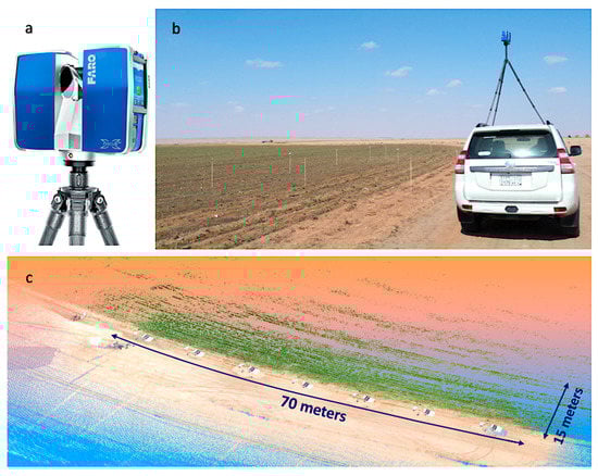
Figure 3.
(a) FARO Focus X330 system used for validating the UAV crop height retrievals; and (b) its scanning location. To provide an adequate view angle of the edge of the field, the LiDAR has been mounted on a 4WD. A network of wooden sticks was deployed around the perimeter of the grids, whose coordinates were used for georeferencing; (c) FARO SCENE software representation of the seven scan grids performed at about 10 m distance from each other, allowing for the reconstruction of a reasonably wide area of the field. The scan grids retrieved on 9 May clearly show the “blocking effect” caused by the first crop, producing an incomplete point cloud at further distances.
The average point spacing was set at 1.2 cm at 10 m distance. For all the LiDAR surveys, a network of seven wooden stakes was deployed around the perimeter of each scan grid (seven for each campaign) and their location was recorded using the RTK-GPS system. These measurements were then employed for point cloud registration in the FARO SCENE (Version 5.3) proprietary software package for georeferencing, which joins together the multiple scans into a unique cluster, for a total of about 70 m in length (Figure 3c). The area of the scans within the perimeter of the GCPs was extracted and processed further using code written in-house. The scanned grids were georeferenced and the 4 April terrain model (LiDAR bare soil) was subtracted from the DSM to determine the crop height for each scan grid.
To enable the crop height comparison, the exported LiDAR point clouds from the FARO software (with the elevation coordinates of each grid point) were imported into ArcGIS Desktop (Version 10.3.1) and converted to vector point data. Interpolation with an inverse distance weighting algorithm was then applied, hence retrieving the raster representing the digital surface model at the same resolution as the SfM dataset to facilitate a cell by cell comparison. While the point cloud density of the LiDAR data is not changing at the different resolutions (i.e., we just average the result at 2.5, 5, 10 and 20 cm), the UAV density outcomes are different at every resolution scale, as the processing workflow is undertaken separately for each of them. The LiDAR scans were collected during each field campaign excluding the last one, since the scanning angle of the instrument was not sufficient to capture the density and height of the vegetation at the end of the growing season. As such, four unique datasets were used to assess the accuracy and performances of the UAV-based SfM methodology (Section 2.3). All the LiDAR scans were recorded the same day (and close in time) to the UAV flights, hence providing a reliable evaluation dataset. For the ground comparison, LiDAR data from an earlier scan (4 April 2016) were used, while the dynamic crop height comparison relied on the UAV coincident LiDAR scans. To account for the lower scan density at the edge of the LiDAR scans and for the scanning angle intrinsic in the LiDAR system, the comparison undertaken here is based upon the evaluation of a 50 m × 15 m area that was extracted from the overall collected LiDAR point cloud (approximately 70 × 20 m area).
Linear regression comparison analysis was performed between the LiDAR and SfM derived ground and plant height gridded dataset. The root mean square error (RMSE), relative root-mean-square error (rRMSE), coefficient of determination (R2) and the mean absolute variation (MAE) were used to assess the performance of the UAV-SfM technique in estimating crop height across the maize field:
where is the covariance between the LiDAR scan values and the UAV retrievals , is the standard deviation, is the mean value of the LiDAR values and is the total number of pixels in each dataset.
3. Results and Discussion
3.1. Crop Height Determination with UAV Point Cloud
The GSD was resolved for the orthomosaic and digital surface elevation, with an average of 15.1 points/cm2 produced in the point cloud. The geolocation error of the generated data (reflected in the RMSE) was calculated using the initial and reconstructed GCP locations and varied between 1.5 and 4 cm over time, representing an acceptable level of accuracy given the ground control point error (<5 cm) and the high resolution of the DSM (~2.5 cm). Figure 4 (top row) presents the derived DSM outputs from Photoscan (gained from the merged and filtered point cloud), together with the crop height level estimates (middle row), retrieved as discussed in Section 2.4, that is, by subtracting the baseline terrain map collected immediately after the crop sowing date (on 4 April), from each subsequent DSM survey. Finally, the pattern of the crop height anomaly around the mean was also evaluated (bottom row).
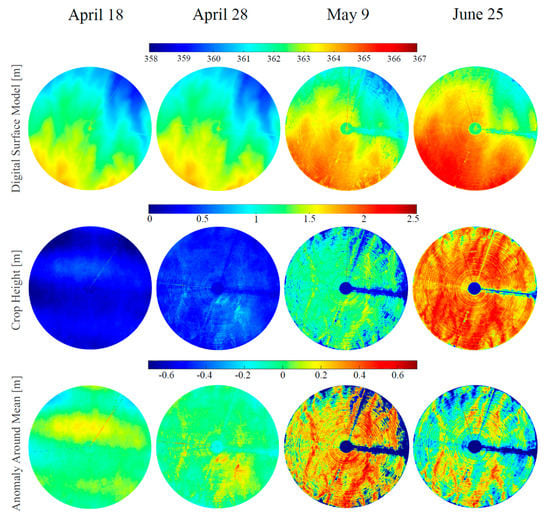
Figure 4.
UAV derived digital surface models (top row) and crop height retrieval (middle row) for each of the campaigns. A rapid crop development from ground level to approximately 2.5 m was captured during the 3 month growth period. (bottom row) shows the anomaly of crop height around their mean values for each UAV survey.
As can be seen in Figure 4, an examination of the retrieved DSM and crop height from the UAV provides considerable insights into the small-scale variability of the crop systems. The UAV-based SfM methodology was able to discriminate areas with both abundant and sparse vegetation (the heterogeneity in the maps highlights this aspect), allowing for the detection of intra-field variability at specific times throughout the crop growing season. Several characteristics of the pivot development can be depicted from the DSM and crop height retrievals. Areas with lower vegetation can be seen throughout the field. Although some areas (stretching to the center) seem to recover by the end of the season (i.e., around the access road on the right of the center pivot), many areas identified as under-performing relative to the field average seem to be maintained in the 25 June scene, including around the perimeter of the field. Certainly, it is likely that vegetation along the periphery of the pivot receives less water from the sprinkler irrigation system due to wind effects and associated spray-losses. Such a vegetation buffer response is noted across many of the pivot systems, with vegetation on the interior of the field faring better than that on the exterior. Additional factors explaining the observed intra-field variability may include: (i) heterogeneity in the soil texture and composition; (ii) chemical properties (i.e., salinity) influencing the growth and development of the crop; and (iii) uneven distribution of irrigation and fertilizer application rates, which are delivered through a combined fertigation system (with possible lower efficiency at the terminal end of the pipe). In this context, regular monitoring of crop dynamics throughout the season represents an important aspect of precision agricultural application and agricultural management decisions (e.g., for irrigation scheduling, fertilizer application and harvesting) [72]. Although some areas still remain under-performing until harvesting date, it is evident from the crop height graphs that no areas within the field get worse (in terms of crop height) during the season, demonstrating a good management practice and the absence of any adverse conditions that may affect specific areas of the pivot (i.e., meteorological events). While evaluation of the temporal intra-field variability of crop status at different growth stages has been reported in previous studies [45,57,58], these analyses were either limited to smaller fields, or used a lower number of flights to characterize the variability.
More detailed information can be inferred from the texture of the DSMs (Figure 4, top row). A wide range in elevation is present within the field, as emphasized by the SW-NE gradient. Indeed, at its maximum, there is a vertical difference of almost 4 m from one side of the field to the other (also verified by the GCP range in Table 1) with a spatial pattern that remains largely unchanged until 28 April. The presence of low (or no) vegetation within the field through the first three UAV campaigns drives this consistency in the spatial pattern of surface elevation. In line with this, the crop height derived on 18 April is characterized by the presence of dark areas in the upper part of the field where the actual height presents some negative values. This is probably caused by the bare soil map (4 April) that raises above the true terrain level, leading to negative height when subtracted from the DSM of 18 April. In practice, although negative values are often removed (as a crop height below zero has no physical meaning), we decided to leave them to highlight the inconsistent retrieval that can arise from typical UAV sensing systems. A better understanding of this behavior can be obtained by examining Figure 4 (bottom row), which plots the anomaly of crop height around the mean value within the field, from which the percentage of crop height localized between a certain range (−0.6:0.6 m) for each UAV campaign was estimated. It should be noted though, that the negative values at 18 April represent only 0.7% of the entire distribution and they are mostly localized in the left and right areas at the top of the field, close to the perimeter (displayed as dark blue areas). It is clear from the localization of these negative regions that this inconsistency is most probably arising from errors due to lower overlap in the UAV imagery at the borders of the flight path compared to its center. This condition affects the number of key points that can be detected between images, producing a point cloud with lower density and therefore, with lower accuracy. Also, as stated in Section 2.2, the flight performed during the second UAV campaign (18 April) was affected by a camera-bay blockage, which required a cropping procedure to remove the dark area over each image. The reduced size (and overlap) of the pictures definitely affected the imagery post-processing, as the vertical size of the image was reduced by almost one quarter of its total length (Table 1).
On 18 April, there are two banded regions in the upper- and lower-middle areas of the field that show positive anomalies above the mean (see bottom row of Figure 4), that do not seem to be maintained in the subsequent campaigns. It should be noted that the crop height retrieved on this date is likely affected by a higher level of uncertainty compared to those in later UAV flights, as the thin structure of the vegetation at the early stage (emergence) is not well captured by the generated point cloud. As reported by Grenzdörffer et al. [46], errors are strongly related to the stage of crop growth. That is, crop height is better determined by the UAV-SfM system if the canopy surface is dense and homogeneous. In early development stages, crop height is more challenging to retrieve as the vegetation cover is lower and the individual stalks are small and do not normally form a closed canopy.
The pattern of the crop height anomaly around the mean (Figure 4, bottom row) is also able to identify areas of higher and lower performances around the field, bringing attention to specific areas that are seen to enhance the growth and development of the maize throughout the season. In particular, the “positive” anomaly captured on 28 April in the S-E part of the field is followed by a similar structure in the next two UAV flight dates, confirming the capacity of that particular area to provide conditions more favorable to crop development (e.g., perhaps driven by better soil nutrient and water content availability). Similar responses are shown for the vertical stripe on the left side of the field, which is also repeated on 9 May and 25 June. Such improved crop height response in these particular zones may be a consequence of a different soil texture, type or salinity properties, which led the plants to be higher than the crop height average: by up to 75 cm on 9 May and 62 cm on 25 June. A closer examination of the last two campaigns indicates that the anomaly around the mean is more emphasized on 9 May rather than on 25 June, demonstrating a stabilization in terms of average height within the field during the last month of the growing season. Based on the growth trend of the crop, the penultimate field campaign matches the flowering period, after which the canopy structure is subject to an increased density (with expanding leaves and corn cob) rather than any significant rise in height. This period between image collections could have given the plants time to stabilize in terms of height, producing a smaller anomaly compared to the previous campaign.
To highlight the ability of the SfM to retrieve fine structural changes in crop height, three sub-areas of 30 m × 30 m were extracted from within the field and presented in Figure 5. A healthy crop (Area 1), a static no-crop region (Area 2) and a problematic area (Area 3), were retrieved throughout the growing season, with changes in crop coverage and plant height depicted over the sampling dates. Perspectives from Areas 1 and 3 illustrate that the crop canopies were adequately reproduced by the point clouds, with crop growth well captured across the different stages. Visual interpretation of the images in Figure 5 reflects the spatial agreement between the derived crop height and the underlying orthomosaic, confirming the efficiency and accuracy of the UAV-SfM approach. As can be seen, Area 1 depicts a relatively stable canopy coverage for all dates, especially when compared with Area 3, which shows the impacts of soil or irrigation-related problems on the canopy structure. Further examination indicates that Area 1 and 3 follow the same growth trend up until 28 April, after which the crop development and subsequent canopy response diverge. For instance, by 9 May, Area 3 shows a loss in canopy structure, with half of the area of the 3D model and underlying orthomosaic reflecting the low canopy structure (although this is partly recovered by the time of the last retrieval on 25 June). Area 1 on the other hand, manifests a more linearly increasing crop height trend and is absent of any significant canopy alterations throughout the season. As expected, Area 2 remains consistent throughout the UAV collection period, reproducing the static bare soil section in the center of the pivot.
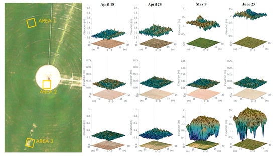
Figure 5.
Dynamic crop height retrievals for three different sub-areas in the maize field, including: a healthy region (Area 1), a static bare-soil region (Area 2) and an affected region (Area 3). The displayed orthomosaic in the left panel, from which the areas are depicted, was derived from the UAV survey on 9 May.
The dynamic crop height across the entire field was also visualized by considering the histograms of all pixel-based elevations for each of the individual UAV campaigns. The histograms were constructed by placing each z-coordinate of the crop surface models in a bin-size of 1 cm, providing an accurate representation of the distribution and frequency of the crop height estimates. As can be seen from Figure 6, the time-evolution of plant height is apparent across the growing season. The early stage distribution from 18 and 28 April, presents a sharp peak and narrow Gaussian distribution, reflecting the low crop height (25–50 cm) characteristic of the maize field at the beginning of the growth cycle. In the case of these low canopy retrievals, it can be observed that the distribution depicts some negative values in the field for the April 18 campaign, suggesting some inconsistency in the results. As stated before, negative values of crop height were obtained because ground values in the first campaign had higher elevation compared to those created on 18 April, thereby leading to negative height in the derived crop surface model. For this particular date, the crop coverage within the field is still low and the captured bare soil is almost the same as the previous campaign (4 April). However, any error in the UAV GPS coordinates, even though these have been corrected through the introduction of GCPs, still presents as a source of uncertainty, ultimately producing lower crop height estimates relative to the first survey (4 April). The plant height corresponding to the last two UAV surveys (9 May and 25 June) shows the highest intra-field variability, reflected by lower peaks and a wider range of the distribution: from 0 to 1.6 m and from 0 cm to 2.35 m, for the respective campaigns. Despite the similarity in the distribution of the last two UAV campaigns, 9 May shows a bimodal distribution that is not present on 25 June. This is explained by the presence of areas with low vegetation and with heights less than 50 cm, which represent 11.3% of the values in the distribution. On the other hand, 77% of the field has a height above 0.992 cm, which represents the average crop height. This intra-field variability, clearly depicted in the histogram, is also emphasized in calculations of the 25th and 75th percentile, whose values are 0.914 cm and 1.30 cm, respectively.
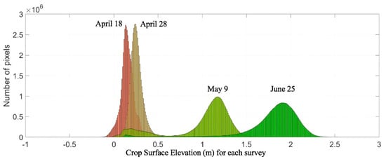
Figure 6.
Dynamic crop height estimation throughout the maize growing season. The multiple histograms represent the retrieved crop height for each of the UAV campaigns.
Interestingly, it can be noted that the crop growth occurring in the two-weeks between 28 April and 9 May (i.e., about 1 m in height) represented a more rapid height development relative to the following month and a half between 9 May and 25 June (about 60 cm). The fast crop development after 28 April, which may explain (in part) the high spatial variability captured by the fixed-wing UAV on 9 May, is further confirmed by the differences in the median values recorded from the last three campaigns: 0.25 cm, 1.20 cm and 1.86 cm.
The typical length of the maize season in the study region usually ranges between 70 and 90 days, depending on the sowing date as well as climatic and environmental variables [73,74]. Indeed, the timing of crop phenology from one growth stage to another (development periods) is directly affected by temperature changes [75,76,77] and it is strongly correlated with the cumulative daily temperature [78] (i.e., degree days). Generally, cool temperatures tend to slow down growth, while warm temperatures hasten maturity [74,79]. The rapid development of crop height that occurs between 28 April and 9 May reflects the crop reaching the end of its vegetative stage, which starts approximately two weeks before flowering (around 9 May in our case) [80,81]. During this rapid growth phase, the stalk follows a substantial development, leading plant height to increase dramatically [82].
Being able to track crop growth at the intra field scale provides an important metric with which to understand and assess the multiple developments that can occur in diverse areas within a field of such size. From this, specific management decisions can be implemented to improve the response of problematic crop areas, hence reducing the risks of potential yield losses. Timely and accurate prediction of crop height during the growing season is important in farm management, as it can be used by farmers and operators for improved decision-making [83] and by government and researchers agencies for informing food security policies [84]. Further assessment of the accuracy of these retrievals is provided below.
3.2. Evaluation of UAV-Based Retrievals with LiDAR Scans
How accurately the digital surface model and baseline terrain map are able to be determined by the UAV-SfM technique is critical to the accurate determination of crop height. Therefore, an evaluation procedure is needed for assessing the UAV-SfM reconstructions. In the following, a comparison between UAV and LiDAR scan data is presented, providing a mechanism to assess the accuracy of both bare soil and digital surface model retrievals (from which the crop height is extracted). Despite the higher spatial coverage of the fixed-wing UAV system, which allows for the survey of an entire 50 ha field in a single flight, the ground-based LiDAR system provides a higher point density and accuracy but over a much smaller area. A pixel-by-pixel comparison between the two datasets is performed, with varying numbers of measurement (i.e., pixel-height) analyzed based on the sampled resolution (i.e., 1,269,822; 317,455; 79,364; and 19,892 pixels were considered in dataset comparisons at 2.5, 5, 10 and 20 cm, respectively). Figure 7 presents a summary of the UAV and LiDAR retrievals for the bare soil surface acquired on 4 April.
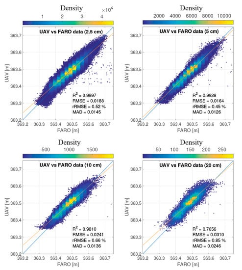
Figure 7.
Density scatter plots illustrating the ability of the UAV and the LiDAR systems in reproducing the digital terrain model at 2.5, 5, 10 and 20 cm resolution (from top left to bottom right). The ground comparison is referred to the first UAV campaign on 4 April, where a 50 by 15 m area was selected as a sample for assessing the accuracy of the UAV-SfM system.
Overall, the UAV-SfM results represented in the density scatter plots show very good correlation and low RMSE (few centimeters) at the four different resolutions. In all cases, the data are consistently retrieved and distributed around the 1:1 line. The 5 cm resolution result presents the lowest bias compared with the other three resolution retrievals, each maintaining a fairly consistent positive bias of approximately 5 cm. However, in all cases, the SfM elevation was slightly higher than the corresponding LiDAR values, which is most likely explained by errors in the SfM point cloud reconstruction and in the ground measurements [47]. As expected, the highest correlation was obtained for the data at 2.5 cm and 5 cm (r2 = 0.99), followed by the 10 cm (r2 = 0.98). The worse correlation was determined for the 20 cm (r2 = 0.77), which also presents the highest value of RMSE, at 3.1 cm. RMSE values for the 2.5 and 5 cm retrievals show a well contained error, with a range that varies between 1.6 and 1.8 cm, while 10 cm resolution was only slightly higher (2.4 cm). The mean absolute error (MAE) and the relative root-mean-square error (rRMSE) further reinforce this response, with an observed range amongst the pixel-by-pixel comparisons between 0.0126 and 0.0246 cm for the MAE and 0.45% and 0.85% for the rRMSE.
Overall, these results clearly illustrate the ability of the UAV-SfM approach to accurately model the terrain surface elevation, which is critical for a reliable extraction of the crop height values. Employing a different point cloud density, hence producing different resolution scales (i.e., obtained from resolution-specific processing at each scale), did not particularly affect the results, whose accuracy is maintained even at a lower level of detail (i.e., 10 cm). It should be noted that while the results are only marginally different (in terms of correlation) using 2.5, 5 and 10 cm resolution, employing coarser resolution (i.e., 20 cm) data reduces the reliability of the dataset, having an r2 of 0.77. The reduced point cloud density obtained at 20 cm most likely explains the difference between the correlations obtained at the other resolutions. The correlation between the baseline terrain map retrieved with the UAV-based SfM approach and the LiDAR point cloud was also assessed by Malambo et al. [32], who confirmed the importance of an accurate terrain map to extract reliable crop height. Also in that study, high values of the coefficient of correlation were achieved (0.88–0.97), although fewer measurements were utilized for the statistical comparison (n = 380), as a result of a raster grid interpolation.
During the course of crop development, vegetation growth is not a continuous or linear phenomenon but follows a series of generally well-defined crop stages [81]. In the early development phase (emergence stage), the height of the crop is challenging to retrieve, as the vegetation density is low and lacking a closed canopy structure. Hence, UAV technologies will generally struggle to identify small stems and leaves, especially if the flight altitude is high (such as in this case, at more than 100 m). From an optical sensing perspective, the resolvable resolution in these conditions can result in a poor discrimination of vegetation from the underlying ground surface, resulting in a relatively homogeneous response signal. Furthermore, if the crop structure is either sparse or particularly thin, the UAV will deliver a lower crop height compared to the LiDAR. This “height dampening” is a consequence of the filtering step embedded in the SfM algorithms [58], which smooths out the solution, hence leading to a poorer identification of single plants in the emergence stage. As the crop density and structure change during the development stages, crop height should be resolved with an increasing level of accuracy. The challenging retrieval of crop height in early development stages has been highlighted by Grenzdörffer et al. [46], who considers the UAV-SfM limitation increasing at coarser resolution because within a single pixel, portions of one or multiple plants (and their shadows) merge into one single signal (canopy level). In Shi et al. [47], the weak correlation between UAV estimates and ground truth was found to be a result of the inadequate image resolution, which was not able to distinguish the small tassels on top of the plants, that were measured on the ground. Furthermore, Bendig et al. [42] and Malambo et al. [32] pointed out the lower fidelity of the UAV-SfM system as a consequence of the restricted viewing perspective (nadir angle), which does not allow for a full 3D reconstruction of the canopy.
Following these considerations and the similarity in the statistical results achieved for the terrain base map at the four different GSDs, we carry out a subsequent evaluation of retrieved crop height using the same resolution scales, with the aim of testing their accuracy in providing the necessary intra-field variability: a key requirement for any precision agriculture based approach. For this purpose, the same portion of the field evaluated in the bare soil analysis, is now considered for crop height estimation on the penultimate UAV campaign (9 May), where the crop height variability is much more noticeable. It should be noted that due to the “blocking effect” caused by the first crop (see Section 2.4 for more details), some small areas at further distances could not be fully represented by the LiDAR scanned point cloud, hence generating “No Value” at those particular locations. For consistency in the UAV/LiDAR comparison of the results, the pixels of the UAV crop height map located at the same coordinates of the LiDAR “No Value,” have been removed. Figure 8 shows a pixel-by-pixel comparison of the UAV and LiDAR systems, which are reported in density scatter plots, while the comparison of their crop height maps is presented in Figure 9. From our analysis, UAV-based crop height retrievals are shown to be quite reliable in detecting the variability within the considered area at the edge of the field. The pattern of the crop, depicted in the underlying maps (Figure 9), is accurately predicted by the UAV system, which is also able to distinguish the adjacent crop rows that are separated by about 50 cm from each other. From these analyses, the heterogeneity in the vegetation along the periphery of the pivot is clearly impacted relative to the pivot average, with losses in canopy structure that are most likely explained by reduced irrigation efficiencies at the terminal end of the sprinkler system (see Section 3.1 for more details). It should be noted that scatter plots and crop height maps clearly represent two distinct distributions: the majority being bare soil, which is reflected by a high density area in the scatter plots (in yellow, where the height is nearly close to zero) and a smaller proportion being crop, which presents a linear trend with similar values for both UAV and LiDAR.
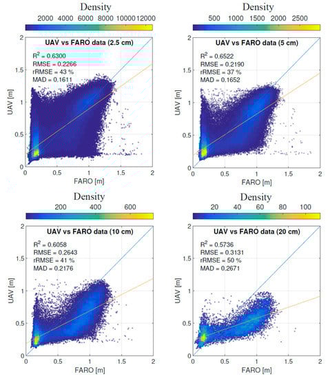
Figure 8.
Density scatter plots comparing the UAV-SfM approach crop height retrievals and the LiDAR scanned point cloud. From top left to bottom right, the panels show the 2.5, 5, 10 and 20 cm resolution from the UAV campaign of 9 May.
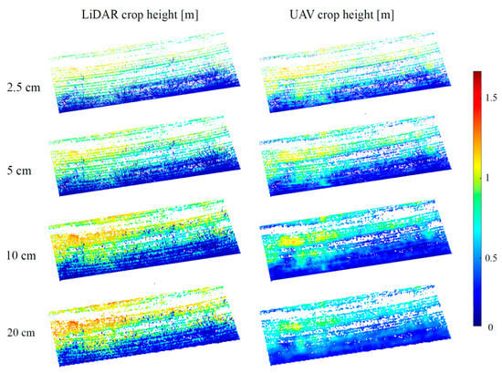
Figure 9.
50 by 15 m crop height maps generated from both LiDAR (left column) and UAV (right column) systems, with clear identification of intra-field variability. Resolution of 2.5, 5, 10 and 20 cm have been assessed (from top row to bottom row).
In terms of error, the high values of the rRMSE (with a range between 37% and 50%), are therefore the consequence of these different (and multiple) distributions in the scatter plots. As expected, the significant differences in crop structure within the area are better delineated using higher resolutions (i.e., GSD of 2.5 and 5 cm), which also produce the lowest RMSE (0.21 cm–0.22 cm). The solution at 10 cm seems to produce a less similar pattern to that generated by the LiDAR, which further worsens when using a 20 cm GSD. However, good similarity in crop height is reflected in the correlation indices of the density scatter plots (Figure 8), with values of 0.57 at 20 cm resolution, 0.60 at 10 cm and 0.62 and 0.65 using 2.5 cm and 5 cm GSD, respectively.
In general, all the resolution scales generate lower crop height estimates compared to the LiDAR, reflecting the “height dampening” typical of the SfM filtering process [58]. Although a negative bias is clearly visible at every resolution scale, the crop height above 0.5 m seems to be accurately predicted by the UAV systems, with values that remain close to the 1:1 line in all cases, albeit with some evident underestimation by the UAV system across all resolutions. It can be noted that a gradual reduction of the maximum crop height detectable by the UAV is present from 2.5 to 20 cm. In particular, the highest values of crop height (1.4 m) are retrieved using a 2.5 cm GSD, whilst the solution at 20 cm only managed to detect values up to 1 m height. This gradual reduction can be explained by the heavier height dampening factor produced by averaging the point cloud over a larger area (i.e., 20 cm).
Interquartile statistics of the two datasets plotted in Figure 8, show that the 75th percentile of 2.5, 5, 10 and 20 cm GSD are 2.7, 9.3, 21.2 and 30 cm lower than the LiDAR, while the 25th percentile are 9.2, 11.3, 21.7 and 23.1 cm higher, testifying to a reduced range in the UAV crop height estimation. While the lower 75th percentiles may be explained by the smoothing effect embedded in the SfM algorithms, the higher 25th percentiles are likely explained by a reduced capacity of the UAV system in retrieving the smallest and thinnest plants, which present the lowest crop heights [46]. However, although the UAV lacks the capacity to effectively retrieve the outliers (i.e., the min and max crop height), it provides a fairly strong correlation, even at courser resolution (10 cm GSD).
A further discussion can be made from Figure 8, where a vertical feature is present on the left side of all the scatter plots. The UAV-SfM approach is generating crop height values up to and over 1 m, while the LiDAR system is not. One main source of discrepancy can be represented by unstable data acquisition conditions. As previous studies have explained [46], the vegetation surface should be stationary during the aerial survey to ensure a successful image matching in post-processing and a highly accurate positioning determination. Nevertheless, in most agricultural environment, wind effects are a key factor influencing retrieved imagery [85]. Crop movement due to high winds impacts the quality of the imagery by introducing positional error, since the same feature of the crop can be recorded in different positions. In addition, errors in the vertical crop height are most common during the later growth stages when the plants are taller and may be slanted during wind condition [31]. Records from the farm weather station, reported that the wind speed at the time of the UAV flight on 9 May (10:30 a.m.), was about 10 km/h, which can partially explain the errors in the UAV retrievals. As shown in Figure 9, the UAV at the highest resolutions (i.e., 2.5 and 5 cm) was able to distinguish the crop rows and the adjoining soil. The wind effect during the time of the flight may have bent some of the plants, which consequently covered the adjacent soil pixels. As a consequence, the UAV can retrieve higher values, as shown in the scatter plots. Another source of uncertainty is represented by small geolocation errors that could also have affected the reliability of the results, especially at the higher resolution (i.e., 2.5 cm). It should be noted that a UAV versus LiDAR pixel-by-pixel comparison at such a high resolution has not previously been reported in the literature. Similar evaluations of UAV derived crop height against LiDAR point cloud have relied on either an interpolation of the LiDAR data onto a 2 m grid [32], or averaging the crop height onto a 0.3 m [57] or a 0.5 × 0.6 m grid [56], resulting in comparatively few measurements for the evaluation, relative to the present study. The correlation obtained between LiDAR and UAV plant height is consistent with previous findings in maize [32] and barley [57]. In line with these studies, a better correlation has been obtained between crop height measurements at the flowering stage, confirming that imagery captured at the end of the stalk elongation (flowering stage) is better correlated with ground truth data [86].
As Figure 9 shows, crop height can vary considerably within the same field, even though irrigation and fertilizer application are applied with a consistent management practice across the pivot. However, other conditions can also influence the observed intra-field variability. These conditions can be quite variable and involve natural fluctuations in biological and plant physiological processes, soils and climate, all of which influence production levels and ultimately, potential profit at the farm gate. However, they are also impacted by ineffective irrigation practices, fertilizer variability, salinity and other soil property issues, as well as the decision-making skills of the farmer. Being able to “scout” for these intra-field issues offers insight not only for yield prediction but also in taking remedial action to address changes as they appear. When combined with GPS technology commonly deployed on farm equipment, such information can help guide the delivery of agricultural inputs to increase yield and the profitability of crops. While UAVs may provide the capacity to deliver such guidance, they also come with some caveats, some of which are discussed in the following section.
3.3. Application and Limitations
The dynamic estimation of the maize crop height was monitored quite accurately by the fixed-wing UAV throughout the growth cycle. While some previous studies have highlighted the limitation of poor point cloud generation by the UAV-SfM technique in landscapes where vegetation was dense and complex (i.e., dead or dry bushes with many overlapping branches in coastal areas) [87,88] as well as in maize crop monitoring [89], the work presented here provides additional insights on the structural variations within deep canopies. Results suggest that the UAV-SfM technique performs reasonably well in terms of reproducing the canopy cover at later stages of the growing season (flowering and maturity) and when complex crop structure and density increase. The comparison of the retrieved DSM, from which the crop height maps were generated, revealed some of the issues with the UAV-based retrievals: especially in reproducing the vegetation at early stages of development. In these cases, the UAV-based SfM approach generates a point cloud that struggles to detect the small-scale plant structure but which is captured by the LiDAR system. While one solution to this would be to reduce the flight altitude of the UAV (to obtain a higher resolution), current technologies still demand a compromise between areal coverage and flying height, due to power and related flight time constraints. In an ongoing (but unrelated) study, a lower flight height (20 m) and higher resolution (0.5 cm) digital surface model was able to distinguish leaves and fruit within a single plant, providing considerable insight on the health and condition of the vegetation. However, the covered area was limited to 0.5 ha due to the low flying speed of the rotary UAV, which was required to generate sufficient overlap between the images at such altitude and due to power supply constraints that kept flights to less than 30 min. The limited area coverage that characterizes rotary UAV versus fixed-wings systems represents an issue for precision agricultural application at larger scales (i.e., commercial scale monitoring). Because of the lower cruise speeds typical of rotary UAVs, an increased flight altitude (relative to that used in this study) would be necessary to cover the same 50 ha agricultural field in a single flight. However, this would also result in a coarser resolution retrieval (i.e., larger GSD) unsuitable for precision agricultural purposes. While LiDAR onboard a UAV could undoubtedly increase the level of detail with which a crop can be retrieved [90], obtaining crop height (and hence crop status and intra field variability information) using relatively cheap instrumentation with a good level of accuracy remains a priority to encourage broad user-uptake. In this context, to improve the accuracy of the UAV systems retrieval, Harwin et al. [87] suggested to perform the RGB data collection from multiple points of view. Although this allows a more reliable 3D reconstruction of the dense cloud, it would dramatically increase the time required for the data collection and subsequent processing.
A more generic limitation to the UAV based retrievals is the computational cost involved in image processing. In this study, the time needed to generate a final crop height map can be considerable: up to 2.5 days if an ultra-high resolution of 2.5 cm is required. These times decrease to 24 h, 9 h and 6 h for 5 cm, 10 cm and 20 cm, respectively. It should be noted that the processing undertaken here was achieved using a high-performance server (16 core, 2.4 GHz and 128 Gb RAM server workstation), which delivers solutions at a much faster rate compared to a standard desktop system. For a rapid assessment of the field variability and condition of the crop, an efficient but still accurate methodology is required. Certainly, it is not feasible for a farmer or farm manager to reproduce the type of processing performed herein, especially if they are to manage the multiple fields of a commercial-scale concern. While tuning the resolvable resolution provides some computational relief (by a factor of 7; see Section 2.3), it remains impractical to suggest this as an operational methodology in a real world scenario.
In providing some practical guidance, the employed SfM approach is able to deliver insights into intra-field crop variability with relatively good accuracy and timing at a 10 cm GSD. While higher resolutions result in improved insights, these come at the cost of an unacceptable processing time. It should be noted that the SfM workflow can deliver a 10 cm resolution product by lowering the accuracy in the point cloud generation (hence reducing the processing time). In practice, the same resolution could be achieved with a UAV flight performed at 500 m altitude but which would be challenging for both safety and operational reasons due to increased risk of wind effects and line of sight restrictions. This represents an important aspect of the fixed-wing UAV-based SfM approach described herein, which can provide precision agricultural solutions as needed and in a timely manner.
4. Conclusions
The study presents an evaluation of a fixed-wing UAV-based SfM technique to retrieve the 3D structure of a 50 ha maize crop at the commercial field scale. Imagery collected from a UAV were used to reconstruct Digital Surface Models (DSM) and orthomosaics over five distinct dates throughout the growth cycle from which crop height was extracted. Results from this analysis show that the methodology is able to reproduce the observed spatial variability of the crop height within the maize field across all crop development stages. Comparison against LiDAR point clouds shows that UAV-SfM data were in good agreement, with a correlation up to 0.99 and RMSE 0.0164 cm for retrieving ground surface elevation after sowing (4 April). For the estimation of absolute crop height at flowering time (9 May), when complex structure and high intra-field variability of the maize crop were present, correlations of 0.65 and RMSE of 0.21 cm were obtained.
Despite these positive results, further improvements in image collection and processing [1,91,92] are required to reduce bias in the UAV-based SfM retrievals. Also, decreasing the time required for a fast and accurate delivery of precision agriculture solutions is necessary for practical application. The retrieved ground sampling distance represents a compromise between physical constraints of flying height (and thus flying time) and areal coverage, together with more practical considerations such as providing information about the status of the crop within the field relatively quickly (i.e., processing time) and with the necessary accuracy (retrieval fidelity). Our results demonstrate that the use of a 10 cm resolution product represents a suitable compromise between accuracy and processing time, delivering a reliable product with a processing time of approximately half a day.
Sustained growth in agricultural productivity represents one of the anchors of food security [93] and shortfalls in farm food production need to be efficiently addressed in order to ensure increased yield [94]. Frequent temporal observations of crop height aid in this effort but traditional manual methods to assess intra-field crop status are time consuming and impractical to perform at scale. Proximal remote sensing approaches offer a clear alternative to rapid identification or early detection of problems within a field. As illustrated here, high-resolution UAV-based data can be readily employed to reliably extract details on the status and development of crops on a taskable basis, informing the implementation of precision agriculture applications. From a practical perspective, the observable variations in crop behavior represent valuable information that can aid farmers in improving or tailoring management responses.
Author Contributions
M.F.M. and S.D.P. conceived and designed the experiment. S.D.P. performed the data collection. M.G.Z. analyzed the data and compiled the results. M.G.Z. wrote the paper with the assistance of M.F.M. and I.H. All authors discussed the results and contributed to writing and editing the submitted manuscript.
Funding
Research reported in this publication was supported by the King Abdullah University of Science and Technology (KAUST).
Acknowledgments
We greatly appreciate the logistical, equipment and scientific support offered to our team by Alan King and employees of the Tawdeehiya Farm in Al Kharj, Saudi Arabia and to our research scientist Samer K Al-Mashharawi, without whom this research would not have been possible.
Conflicts of Interest
The authors declare no conflict of interest.
References
- Zhang, C.; Kovacs, J.M. The application of small unmanned aerial systems for precision agriculture: A review. Precis. Agric. 2012, 13, 693–712. [Google Scholar] [CrossRef]
- Singh, K.K.; Frazier, A.E. A meta-analysis and review of unmanned aircraft system (UAS) imagery for terrestrial applications. Int. J. Remote Sens. 2018, 39. [Google Scholar] [CrossRef]
- Manfreda, S.; McCabe, M.F.; Miller, P.E.; Lucas, R.; Pajuelo Madrigal, V.; Mallinis, G.; Ben Dor, E.; Helman, D.; Estes, L.; Ciraolo, G. On the use of unmanned aerial systems for environmental monitoring. Remote Sens. 2018, 10, 641. [Google Scholar] [CrossRef]
- McCabe, M.F.; Rodell, M.; Alsdorf, D.E.; Miralles, D.G.; Uijlenhoet, R.; Wagner, W.; Lucieer, A.; Houborg, R.; Verhoest, N.E.; Franz, T.E. The future of earth observation in hydrology. Hydrol. Earth Syst. Sci. 2017, 21, 3879–3914. [Google Scholar] [CrossRef] [PubMed]
- Marqués, P. Aerodynamics of UAV configurations. In Advanced UAV Aerodynamics, Flight Stability and Control: Novel Concepts, Theory and Applications; Wiley: Hoboken, NJ, USA, 2017; p. 31. [Google Scholar]
- Anderson, K.; Gaston, K.J. Lightweight unmanned aerial vehicles will revolutionize spatial ecology. Front. Ecol. Environ. 2013, 11, 138–146. [Google Scholar] [CrossRef]
- Nex, F.; Remondino, F. UAV for 3D mapping applications: A review. Appl. Geomat. 2014, 6, 1–15. [Google Scholar] [CrossRef]
- Whitehead, K.; Hugenholtz, C.H. Remote sensing of the environment with small unmanned aircraft systems (UASs), part 1: A review of progress and challenges. J. Unmanned Veh. Syst. 2014, 2, 69–85. [Google Scholar] [CrossRef]
- Bongiovanni, R.; Lowenberg-DeBoer, J. Precision agriculture and sustainability. Precis. Agric. 2004, 5, 359–387. [Google Scholar] [CrossRef]
- Torres-Sánchez, J.; Peña, J.; De Castro, A.; López-Granados, F. Multi-temporal mapping of the vegetation fraction in early-season wheat fields using images from UAV. Comput. Electron. Agric. 2014, 103, 104–113. [Google Scholar] [CrossRef]
- Peña, J.M.; Torres-Sánchez, J.; de Castro, A.I.; Kelly, M.; López-Granados, F. Weed mapping in early-season maize fields using object-based analysis of unmanned aerial vehicle (UAV) images. PLoS ONE 2013, 8, e77151. [Google Scholar] [CrossRef]
- Torres-Sánchez, J.; López-Granados, F.; De Castro, A.I.; Peña-Barragán, J.M. Configuration and specifications of an unmanned aerial vehicle (UAV) for early site specific weed management. PLoS ONE 2013, 8, e58210. [Google Scholar] [CrossRef]
- Bendig, J.; Yu, K.; Aasen, H.; Bolten, A.; Bennertz, S.; Broscheit, J.; Gnyp, M.L.; Bareth, G. Combining UAV-based plant height from crop surface models, visible, and near infrared vegetation indices for biomass monitoring in barley. Int. J. Appl. Earth Obs. Geoinf. 2015, 39, 79–87. [Google Scholar] [CrossRef]
- Zarco-Tejada, P.J.; González-Dugo, V.; Berni, J.A. Fluorescence, temperature and narrow-band indices acquired from a UAV platform for water stress detection using a micro-hyperspectral imager and a thermal camera. Remote Sens. Environ. 2012, 117, 322–337. [Google Scholar] [CrossRef]
- Berni, J.A.; Zarco-Tejada, P.J.; Suárez, L.; Fereres, E. Thermal and narrowband multispectral remote sensing for vegetation monitoring from an unmanned aerial vehicle. IEEE Trans. Geosci. Remote Sens. 2009, 47, 722–738. [Google Scholar] [CrossRef]
- Hoffmann, H.; Nieto, H.; Jensen, R.; Guzinski, R.; Zarco-Tejada, P.; Friborg, T. Estimating evaporation with thermal UAV data and two-source energy balance models. Hydrol. Earth Syst. Sci. 2016, 20, 697–713. [Google Scholar] [CrossRef]
- Wallace, L.; Lucieer, A.; Watson, C.; Turner, D. Development of a UAV-lidar system with application to forest inventory. Remote Sens. 2012, 4, 1519–1543. [Google Scholar] [CrossRef]
- Wallace, L.; Musk, R.; Lucieer, A. An assessment of the repeatability of automatic forest inventory metrics derived from UAV-borne laser scanning data. IEEE Trans. Geosci. Remote Sens. 2014, 52, 7160–7169. [Google Scholar] [CrossRef]
- Falster, D.S.; Westoby, M. Plant height and evolutionary games. Trends Ecol. Evol. 2003, 18, 337–343. [Google Scholar] [CrossRef]
- Moles, A.T.; Warton, D.I.; Warman, L.; Swenson, N.G.; Laffan, S.W.; Zanne, A.E.; Pitman, A.; Hemmings, F.A.; Leishman, M.R. Global patterns in plant height. J. Ecol. 2009, 97, 923–932. [Google Scholar] [CrossRef]
- Hunt, R. Plant Growth Curves. The Functional Approach to Plant Growth Analysis; Edward Arnold Ltd.: London, UK, 1982. [Google Scholar]
- Li, D.; Liu, H.; Qiao, Y.; Wang, Y.; Cai, Z.; Dong, B.; Shi, C.; Liu, Y.; Li, X.; Liu, M. Effects of elevated CO2 on the growth, seed yield, and water use efficiency of soybean (Glycine max (L.) Merr.) under drought stress. Agric. Water Manag. 2013, 129, 105–112. [Google Scholar] [CrossRef]
- Shouzheng, Z.Q.L.Y.T. Tree height measurement based on affine reconstructure. Comput. Eng. Appl. 2005, 31, 006. [Google Scholar]
- Yin, X.; McClure, M.A.; Jaja, N.; Tyler, D.D.; Hayes, R.M. In-season prediction of corn yield using plant height under major production systems. Agron. J. 2011, 103, 923–929. [Google Scholar] [CrossRef]
- Law, C.; Snape, J.; Worland, A. The genetical relationship between height and yield in wheat. Heredity 1978, 40, 133. [Google Scholar] [CrossRef]
- Shrestha, D.; Steward, B.; Birrell, S.; Kaspar, T. Corn Plant Height Estimation Using Two Sensing Systems; ASABE Paper; ASAE: St. Joseph, MI, USA, 2002. [Google Scholar]
- Ehlert, D.; Adamek, R.; Horn, H.-J. Laser rangefinder-based measuring of crop biomass under field conditions. Precis. Agric. 2009, 10, 395–408. [Google Scholar] [CrossRef]
- Zhang, L.; Grift, T.E. A lidar-based crop height measurement system for miscanthus giganteus. Comput. Electron. Agric. 2012, 85, 70–76. [Google Scholar] [CrossRef]
- Gul, S.; Khan, M.; Khanday, B.; Nabi, S. Effect of sowing methods and NPK levels on growth and yield of rainfed maize (Zea mays L.). Scientifica 2015, 2015, 198575. [Google Scholar] [CrossRef] [PubMed]
- Araus, J.L.; Cairns, J.E. Field high-throughput phenotyping: The new crop breeding frontier. Trends Plant Sci. 2014, 19, 52–61. [Google Scholar] [CrossRef] [PubMed]
- Chang, A.; Jung, J.; Maeda, M.M.; Landivar, J. Crop height monitoring with digital imagery from unmanned aerial system (UAS). Comput. Electron. Agric. 2017, 141, 232–237. [Google Scholar] [CrossRef]
- Malambo, L.; Popescu, S.; Murray, S.; Putman, E.; Pugh, N.; Horne, D.; Richardson, G.; Sheridan, R.; Rooney, W.; Avant, R. Multitemporal field-based plant height estimation using 3D point clouds generated from small unmanned aerial systems high-resolution imagery. Int. J. Appl. Earth Obs. Geoinf. 2018, 64, 31–42. [Google Scholar] [CrossRef]
- Wang, L.; d’Odorico, P.; Evans, J.; Eldridge, D.; McCabe, M.; Caylor, K.; King, E. Dryland ecohydrology and climate change: Critical issues and technical advances. Hydrol. Earth Syst. Sci. 2012, 16, 2585–2603. [Google Scholar] [CrossRef]
- Famiglietti, J.S. The global groundwater crisis. Nat. Clim. Chang. 2014, 4, 945. [Google Scholar] [CrossRef]
- Wada, Y.; Bierkens, M.F. Sustainability of global water use: Past reconstruction and future projections. Environ. Res. Lett. 2014, 9, 104003. [Google Scholar] [CrossRef]
- McCabe, M.F.; Houborg, R.; Lucieer, A. High-resolution sensing for precision agriculture: From earth-observing satellites to unmanned aerial vehicles. In Proceedings of the Remote Sensing for Agriculture, Ecosystems, and Hydrology XVIII, Edinburgh, UK, 26–29 September 2016; International Society for Optics and Photonics: Bellingham, WA, USA, 2016; p. 999811. [Google Scholar]
- Turner, D.; Lucieer, A.; Watson, C. An automated technique for generating georectified mosaics from ultra-high resolution unmanned aerial vehicle (UAV) imagery, based on structure from motion (SfM) point clouds. Remote Sens. 2012, 4, 1392–1410. [Google Scholar] [CrossRef]
- Fonstad, M.A.; Dietrich, J.T.; Courville, B.C.; Jensen, J.L.; Carbonneau, P.E. Topographic structure from motion: A new development in photogrammetric measurement. Earth Surf. Process. Landf. 2013, 38, 421–430. [Google Scholar] [CrossRef]
- Gindraux, S.; Boesch, R.; Farinotti, D. Accuracy assessment of digital surface models from unmanned aerial vehicles’ imagery on glaciers. Remote Sens. 2017, 9, 186. [Google Scholar] [CrossRef]
- Lingua, A.; Marenchino, D.; Nex, F. Performance analysis of the sift operator for automatic feature extraction and matching in photogrammetric applications. Sensors 2009, 9, 3745–3766. [Google Scholar] [CrossRef] [PubMed]
- Lowe, D.G. Distinctive image features from scale-invariant keypoints. Int. J. Comput. Vis. 2004, 60, 91–110. [Google Scholar] [CrossRef]
- Bendig, J.; Bolten, A.; Bareth, G. UAV-based imaging for multi-temporal, very high resolution crop surface models to monitor crop growth variabilitymonitoring des pflanzenwachstums mit hilfe multitemporaler und hoch auflösender oberflächenmodelle von getreidebeständen auf basis von bildern aus UAV-befliegungen. Photogramm.-Fernerkund.-Geoinf. 2013, 2013, 551–562. [Google Scholar]
- Hoffmeister, D.; Bolten, A.; Curdt, C.; Waldhoff, G.; Bareth, G. High-resolution crop surface models (CSM) and crop volume models (CVM) on field level by terrestrial laser scanning. Proc. SPIE 2010, 7840, 78400E. [Google Scholar]
- Tilly, N.; Hoffmeister, D.; Cao, Q.; Huang, S.; Lenz-Wiedemann, V.; Miao, Y.; Bareth, G. Multitemporal crop surface models: Accurate plant height measurement and biomass estimation with terrestrial laser scanning in paddy rice. J. Appl. Remote Sens. 2014, 8, 083671. [Google Scholar] [CrossRef]
- Varela, S.; Assefa, Y.; Prasad, P.V.; Peralta, N.R.; Griffin, T.W.; Sharda, A.; Ferguson, A.; Ciampitti, I.A. Spatio-temporal evaluation of plant height in corn via unmanned aerial systems. J. Appl. Remote Sens. 2017, 11, 036013. [Google Scholar] [CrossRef]
- Grenzdörffer, G. Crop height determination with UAS point clouds. Int. Arch. Photogramm. Remote Sens. Spat. Inf. Sci. 2014, 40, 135–140. [Google Scholar] [CrossRef]
- Shi, Y.; Thomasson, J.A.; Murray, S.C.; Pugh, N.A.; Rooney, W.L.; Shafian, S.; Rajan, N.; Rouze, G.; Morgan, C.L.; Neely, H.L. Unmanned aerial vehicles for high-throughput phenotyping and agronomic research. PLoS ONE 2016, 11, e0159781. [Google Scholar] [CrossRef] [PubMed]
- Watanabe, K.; Guo, W.; Arai, K.; Takanashi, H.; Kajiya-Kanegae, H.; Kobayashi, M.; Yano, K.; Tokunaga, T.; Fujiwara, T.; Tsutsumi, N. High-throughput phenotyping of sorghum plant height using an unmanned aerial vehicle and its application to genomic prediction modeling. Front. Plant Sci. 2017, 8, 421. [Google Scholar] [CrossRef] [PubMed]
- Parkes, S.D.; McCabe, M.F.; Al-Mashhawari, S.K.; Rosas, J. Reproducibility of crop surface maps extracted from unmanned aerial vehicle (UAV) derived digital surface maps. In Proceedings of the Remote Sensing for Agriculture, Ecosystems, and Hydrology XVIII, Edinburgh, UK, 26–29 September 2016; International Society for Optics and Photonics: Bellingham, WA, USA, 2016; p. 99981B. [Google Scholar]
- Weiss, M.; Baret, F. Using 3D point clouds derived from UAV RGB imagery to describe vineyard 3D macro-structure. Remote Sens. 2017, 9, 111. [Google Scholar] [CrossRef]
- Matese, A.; Di Gennaro, S.F.; Berton, A. Assessment of a canopy height model (CHM) in a vineyard using UAV-based multispectral imaging. Int. J. Remote Sens. 2017, 38, 2150–2160. [Google Scholar] [CrossRef]
- De Souza, C.H.W.; Lamparelli, R.A.C.; Rocha, J.V.; Magalhães, P.S.G. Height estimation of sugarcane using an unmanned aerial system (UAS) based on structure from motion (SfM) point clouds. Int. J. Remote Sens. 2017, 38, 2218–2230. [Google Scholar] [CrossRef]
- Torres-Sánchez, J.; López-Granados, F.; Serrano, N.; Arquero, O.; Peña, J.M. High-throughput 3-D monitoring of agricultural-tree plantations with unmanned aerial vehicle (UAV) technology. PLoS ONE 2015, 10, e0130479. [Google Scholar] [CrossRef]
- Hoffmeister, D.; Waldhoff, G.; Korres, W.; Curdt, C.; Bareth, G. Crop height variability detection in a single field by multi-temporal terrestrial laser scanning. Precis. Agric. 2016, 17, 296–312. [Google Scholar] [CrossRef]
- Stanton, C.; Starek, M.J.; Elliott, N.; Brewer, M.; Maeda, M.M.; Chu, T. Unmanned aircraft system-derived crop height and normalized difference vegetation index metrics for sorghum yield and aphid stress assessment. J. Appl. Remote Sens. 2017, 11, 026035. [Google Scholar] [CrossRef]
- Madec, S.; Baret, F.; De Solan, B.; Thomas, S.; Dutartre, D.; Jezequel, S.; Hemmerlé, M.; Colombeau, G.; Comar, A. High-throughput phenotyping of plant height: Comparing unmanned aerial vehicles and ground lidar estimates. Front. Plant Sci. 2017, 8, 2002. [Google Scholar] [CrossRef] [PubMed]
- Bareth, G.; Bendig, J.; Tilly, N.; Hoffmeister, D.; Aasen, H.; Bolten, A. A comparison of UAV-and TLS-derived plant height for crop monitoring: Using polygon grids for the analysis of crop surface models (CSMs). Photogramm.-Fernerkund.-Geoinf. 2016, 2016, 85–94. [Google Scholar] [CrossRef]
- Holman, F.H.; Riche, A.B.; Michalski, A.; Castle, M.; Wooster, M.J.; Hawkesford, M.J. High throughput field phenotyping of wheat plant height and growth rate in field plot trials using UAV based remote sensing. Remote Sens. 2016, 8, 1031. [Google Scholar] [CrossRef]
- Possoch, M.; Bieker, S.; Hoffmeister, D.; Bolten, A.; Schellberg, J.; Bareth, G. Multi-temporal crop surface models combined with the RGB vegetation index from UAV-based images for forage monitoring in grassland. Int. Arch. Photogramm. Remote Sens. Spat. Inf. Sci. 2016, 41, 991. [Google Scholar] [CrossRef]
- Bendig, J.; Bolten, A.; Bennertz, S.; Broscheit, J.; Eichfuss, S.; Bareth, G. Estimating biomass of barley using crop surface models (CSMs) derived from UAV-based RGB imaging. Remote Sens. 2014, 6, 10395–10412. [Google Scholar] [CrossRef]
- Schirrmann, M.; Giebel, A.; Gleiniger, F.; Pflanz, M.; Lentschke, J.; Dammer, K.-H. Monitoring agronomic parameters of winter wheat crops with low-cost UAV imagery. Remote Sens. 2016, 8, 706. [Google Scholar] [CrossRef]
- Moeckel, T.; Dayananda, S.; Nidamanuri, R.R.; Nautiyal, S.; Hanumaiah, N.; Buerkert, A.; Wachendorf, M. Estimation of vegetable crop parameter by multi-temporal UAV-borne images. Remote Sens. 2018, 10, 805. [Google Scholar] [CrossRef]
- Peel, M.C.; Finlayson, B.L.; McMahon, T.A. Updated world map of the köppen-geiger climate classification. Hydrol. Earth Syst. Sci. Discuss. 2007, 4, 439–473. [Google Scholar] [CrossRef]
- El Kenawy, A.M.; McCabe, M.F. A multi-decadal assessment of the performance of gauge-and model-based rainfall products over Saudi Arabia: Climatology, anomalies and trends. Int. J. Climatol. 2016, 36, 656–674. [Google Scholar] [CrossRef]
- Dandois, J.P.; Olano, M.; Ellis, E.C. Optimal altitude, overlap, and weather conditions for computer vision UAV estimates of forest structure. Remote Sens. 2015, 7, 13895–13920. [Google Scholar] [CrossRef]
- Su, L.; Huang, Y.; Gibeaut, J.; Li, L. The index array approach and the dual tiled similarity algorithm for UAS hyper-spatial image processing. GeoInformatica 2016, 20, 859–878. [Google Scholar] [CrossRef]
- Tahar, K.N.; Ahmad, A.; Akib, W.; Mohd, W. Assessment on ground control points in unmanned aerial system image processing for slope mapping studies. Int. J. Sci. Eng. Res. 2012, 3, 1–10. [Google Scholar]
- Tahar, K. An evaluation on different number of ground control points in unmanned aerial vehicle photogrammetric block. ISPRS J. Photogramm. 2013, 40, 93–98. [Google Scholar] [CrossRef]
- Bhandari, B.; Oli, U.; Pudasaini, U.; Panta, N. Generation of high resolution DSM using UAV images. In Proceedings of the FIG Working Week, From the Wisdom of the Ages to the Challenges of the Modern World, Sofia, Bulgaria, 17–21 May 2015; pp. 17–21. [Google Scholar]
- Aguilar, M.; Aguilar, F.; Negreiros, J. Self-Calibration Methods for using historical aerial photographs with photogrammetric purposes. An. Ing. Gráf. 2009, 21, 33–40. [Google Scholar]
- Zhang, S.; Qu, X.; Ma, S.; Yang, Z.; Kong, L. A dense stereo matching algorithm based on triangulation. J. Comput. Inf. Syst. 2012, 8, 283–292. [Google Scholar]
- Houborg, R.; McCabe, M.F. Daily retrieval of NDVI and LAI at 3 m resolution via the fusion of cubesat, landsat, and MODIS data. Remote Sens. 2018, 10, 890. [Google Scholar] [CrossRef]
- El-Sharif, A. Climatic constraints and potential corn production in Saudi Arabia—A study in agroclimate. GeoJournal 1986, 13, 119–127. [Google Scholar] [CrossRef]
- Doorenbos, J.; Kassam, A. Yield response to water. Irrig. Drain. Pap. 1979, 33, 257. [Google Scholar]
- Gordon, R.; Bootsma, A. Analyses of growing degree-days for agriculture in Atlantic Canada. Clim. Res. 1993, 3, 169–176. [Google Scholar] [CrossRef]
- Fisher, J.I.; Richardson, A.D.; Mustard, J.F. Phenology model from surface meteorology does not capture satellite-based greenup estimations. Glob. Chang. Biol. 2007, 13, 707–721. [Google Scholar] [CrossRef]
- Moeletsi, M.E. Mapping of maize growing period over the free state province of South Africa: Heat units approach. Adv. Meteorol. 2017, 2017, 7164068. [Google Scholar] [CrossRef]
- Neog, P.; Bhuyan, J.; Baruah, N. Thermal indices in relation to crop phenology and seed yield of soybean (Glycine max L. Merrill). J. Agrometeorol. 2008, 10, 388–392. [Google Scholar]
- Brown, D.; Bootsma, A. Crop Heat Units for Corn and Other Warm-Season Crops in Ontario; Factsheet Agdex 111/31; Ontario Ministry of Agriculture and Food: Toronto, ON, Canada, 1993.
- Ritchie, S.; Hanway, J.; Benson, G. How a Corn Plant Develops; Special Report No. 48; Iowa State University: Ames, IA, USA, 1986. [Google Scholar]
- Abendroth, L.J.; Elmore, R.W.; Boyer, M.J.; Marlay, S.K. Corn Growth and Development; PMR 1009; Iowa State University Extension: Ames, IA, USA, 2011. [Google Scholar]
- Bitzer, M.; Herbek, J.; Bessin, R.; Green, J.; Ibendahl, G.; Martin, J.; McNeill, S.; Montross, M.; Murdock, L.; Vincelli, P. A Comprehensive Guide to Corn Management in Kentucky; University of Kentucky: Lexington, KY, USA, 2000. [Google Scholar]
- Zhang, N.; Wang, M.; Wang, N. Precision agriculture—A worldwide overview. Comput. Electron. Agric. 2002, 36, 113–132. [Google Scholar] [CrossRef]
- Fischer, R.; Byerlee, D.; Edmeades, G. Crop Yields and Global Food Security; ACIAR: Canberra, Australia, 2014.
- Mesas-Carrascosa, F.-J.; Torres-Sánchez, J.; Clavero-Rumbao, I.; García-Ferrer, A.; Peña, J.-M.; Borra-Serrano, I.; López-Granados, F. Assessing optimal flight parameters for generating accurate multispectral orthomosaicks by UAV to support site-specific crop management. Remote Sens. 2015, 7, 12793–12814. [Google Scholar] [CrossRef]
- Geipel, J.; Link, J.; Claupein, W. Combined spectral and spatial modeling of corn yield based on aerial images and crop surface models acquired with an unmanned aircraft system. Remote Sens. 2014, 6, 10335–10355. [Google Scholar] [CrossRef]
- Harwin, S.; Lucieer, A. Assessing the accuracy of georeferenced point clouds produced via multi-view stereopsis from unmanned aerial vehicle (UAV) imagery. Remote Sens. 2012, 4, 1573–1599. [Google Scholar] [CrossRef]
- Wu, M.; Yang, C.; Song, X.; Hoffmann, W.C.; Huang, W.; Niu, Z.; Wang, C.; Li, W. Evaluation of orthomosics and digital surface models derived from aerial imagery for crop type mapping. Remote Sens. 2017, 9, 239. [Google Scholar] [CrossRef]
- Li, W.; Niu, Z.; Chen, H.; Li, D.; Wu, M.; Zhao, W. Remote estimation of canopy height and aboveground biomass of maize using high-resolution stereo images from a low-cost unmanned aerial vehicle system. Ecol. Indic. 2016, 67, 637–648. [Google Scholar] [CrossRef]
- Anthony, D.; Elbaum, S.; Lorenz, A.; Detweiler, C. On crop height estimation with UAVs. In Proceedings of the 2014 IEEE/RSJ International Conference on Intelligent Robots and Systems (IROS 2014), Chicago, IL, USA, 14–18 September 2014; pp. 4805–4812. [Google Scholar]
- Khanal, S.; Fulton, J.; Shearer, S. An overview of current and potential applications of thermal remote sensing in precision agriculture. Comput. Electron. Agric. 2017, 139, 22–32. [Google Scholar] [CrossRef]
- Shakhatreh, H.; Sawalmeh, A.; Al-Fuqaha, A.; Dou, Z.; Almaita, E.; Khalil, I.; Othman, N.S.; Khreishah, A.; Guizani, M. Unmanned aerial vehicles: A survey on civil applications and key research challenges. arXiv, 2018; arXiv:1805.00881. [Google Scholar]
- Khan, S.; Hanjra, M.A.; Mu, J. Water management and crop production for food security in China: A review. Agric. Water Manag. 2009, 96, 349–360. [Google Scholar] [CrossRef]
- Fan, M.; Shen, J.; Yuan, L.; Jiang, R.; Chen, X.; Davies, W.J.; Zhang, F. Improving crop productivity and resource use efficiency to ensure food security and environmental quality in China. J. Exp. Bot. 2011, 63, 13–24. [Google Scholar] [CrossRef] [PubMed]
© 2018 by the authors. Licensee MDPI, Basel, Switzerland. This article is an open access article distributed under the terms and conditions of the Creative Commons Attribution (CC BY) license (http://creativecommons.org/licenses/by/4.0/).