Abstract
Geosynchronous synthetic aperture radar (GEO SAR) has great potentials in ship surveillance due to its high time resolution and wide swath coverage. However, the remote slant range will result in a very low signal-to-noise ratio (SNR) of echoes that need to be enhanced by long-time coherent integration. The generalized Radon-Fourier transform (GRFT) can realize the coherent integration of moving target under long integration time by jointly parameter searching along range and velocity directions. Unfortunately, in GEO SAR, the very large slant range and long synthetic aperture will cause the curved synthetic aperture trajectory and non-negligible signal round-trip delay, leading to the failure of the traditional slant range and GRFT signal model for moving targets. This paper proposes an improved GRFT-based approach to realize the detection and imaging of moving ship targets in GEO SAR. Firstly, the accurate slant range for moving ship targets is constructed and the GRFT signal is redefined considering the curved trajectory and signal round-trip delay in GEO SAR. Then, GRFT responses to different motion parameters are analyzed. The procedures of moving ship targets detection and imaging in GEO SAR are presented through the detection with coarse-searched motion parameters in GRFT and the following imaging with fine-searched motion parameters based on minimum entropy. Finally, computer simulations verify the proposed GRFT-based method.
1. Introduction
As a kind of all-day, all-weather, high-resolution remote sensing techniques, synthetic aperture radar (SAR) becomes one of the main approaches of ship surveillance [1,2]. Currently, researches on ship surveillance are mainly concentrated on target detection and estimation [3,4,5], multichannel sea clutter suppression [6,7], and target refocusing [8,9].
As is well known, ship surveillance needs high-frequent and large-scale monitoring of vast sea areas. Unfortunately, low earth orbit SAR (LEO SAR) has coarse time resolution (days to weeks) and limited swath coverage (tens to hundreds of kilometers). Although spaceborne multifunctional SAR has been applied in the detection of moving target (such as TerraSAR-X [10] and RADARSAT-2 [11]), achieving the monitoring of ships [12], the further application is limited by the revisiting time and swath width.
Geosynchronous SAR (GEO SAR) runs on the orbit with the orbit height of around 36,500 km [13], which can provide daily coverage for approximately one third of Earth surface. Areas of interest can be observed within the range of every 1.5–2.5 h per day [14]. Thus, GEO SAR has great advantages in ship surveillance over vast ocean area.
Currently, there are growing interests for GEO SAR, which are mainly concentrated on system design and mission planning [15,16,17,18,19,20,21], imaging algorithms [22,23,24,25], ionospheric effects and compensation [26,27,28], and deformation retrieval [29,30,31]. However, there are rarely related researches on detection and imaging of moving ships.
Obviously, due to high time resolution and wide swath coverage, GEO SAR has great potential in monitoring moving ships. However, the remote slant range of GEO SAR will result in a very low signal-to-noise ratio (SNR) of echoes. The defect of low SNR can be compensated for the static target through long time integration [32]. Unfortunately, the parameters of moving targets are unknown, leading to the failure of coherent integration and the resultantly SNR loss. Therefore, traditional detection and imaging methods for moving targets used in LEO SAR and airborne SAR are not suitable for GEO SAR.
Moving targets detection and imaging can be divided into single-channel and multi-channel SAR schemes according to SAR system configuration. Because of the limitation of low SNR, multichannel configuration cannot be realized currently, as it is mainly designed for clutter suppression where ships have higher radar cross section (RCS) against the surrounding sea background (in general, ships has higher backscattering energy as the metallic materials and corner reflection structures [33,34]). Therefore, moving ship detection and estimation can be realized without sea clutter suppression by single-channel SAR scheme, which can be divided into short-time and long-time integration. Short-time integration utilizes the difference of Doppler frequency distribution between moving targets and clutter to achieve moving targets detection [35], such as moving target indication (MTI) and moving target detection (MTD). This kind of methods only integrates signal energy in the same range unit, so it cannot be realized in moving targets detection in GEO SAR where the range migration is much severer even for static target and the energy is dispersed in tens of range units [36,37]. Thus, long-time integration approaches should be employed.
Focus-before-detection (FBD) technique [38] is a kind of novel long-time integration method. It has been applied to maneuvering targets detection [39,40], targets detection under strong clutter background [41,42], estimation of ground target motion parameters [43], etc. FBD can greatly improve SNR by long-time coherent integration, thereby realizing the detection and estimation of weak targets. GRFT [44] is a typical FBD method, which can effectively overcome the coupling between the range walk and phase modulations by jointly searching along range and velocity directions.
However, in GEO SAR, the integration time is at 100 s level, so the trajectory cannot be approximated as a straight line anymore; meantime, its signal round-trip delay is in 0.1 s order, so the platform motion during the signal propagation cannot be ignored. Thus, the curved synthetic aperture trajectory and non-negligible signal round-trip delay will lead to the failure of the traditional slant range model for moving targets, which has been commonly used in LEO and Airborne SAR. The GRFT-based moving ship target detection and imaging method cannot be employed directly.
This paper proposes an improved GRFT-based approach to realize moving ship targets detection and imaging in GEO SAR. The main contributions are as follows: the accurate slant range model for moving ship targets in GEO SAR is established; then, based on the slant range model, the GRFT-based signal integration method is modified and the processing for moving ship targets detection and imaging is given. In the paper, we assume that the moving ship can be focused when there exists the rotation of the moving ship caused by ocean waves. This is under the assumption that the ship has huge inertia and the motion of hull centroid is not affected by ocean waves. The fine analysis of the ocean waves’ influences will be considered in future work.
The paper is organized as follows. In Section 2, the accurate slant range model for moving ship targets in GEO SAR is established and then simplified by analyzing influences of target motion. Subsequently, the GRFT signal model in GEO SAR is modified. In Section 3, responses of GRFT for different motion parameters are analyzed, and then two kinds of motion parameters’ searching intervals (including coarse and fine motion parameters’ searching) are defined. Then, the minimum entropy is used as the moving ship target imaging criterion. The processing of moving ship targets detection and imaging in GEO SAR, which can be summarized as detection with motion parameters’ coarse searching in GRFT and the following imaging with fine-searched motion parameters, is given. In Section 4, simulations are carried out to verify the proposed method. Section 5 concludes the paper.
2. GRFT Model for Moving Ship Targets in GEO SAR
In order to make equations more clearly in this section, the symbol list is given as Table 1.

Table 1.
Symbol list.
2.1. Accurate Slant Range Model
In GEO SAR, the movement of static target with the Earth rotation must be considered. Therefore, the moving target velocity can be expressed as the resultant velocity, which combines the Earth rotation velocity and the velocity of target motion. The moving ship target have a huge inertia, so here we assume its motion is uniform within the integration time [45,46]. is defined as the velocity of ship targets’ motion. The slant range model of moving ship targets considering the curved synthetic aperture trajectory and non-negligible signal round-trip delay, which can be obtained by modifying the slant range model of static targets [47], can be written as
Figure 1 shows the geometry of moving ship targets in GEO SAR. This model takes into account the Earth rotation. Thus, it can be considered that the resultant velocity of moving ship targets can be divided into and .
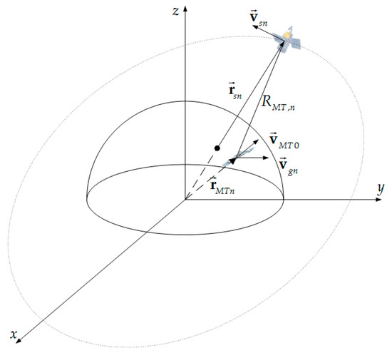
Figure 1.
Geometry of moving ship targets and geosynchronous synthetic aperture radar (GEO SAR).
The slant range of moving targets in GEO SAR can be approximated by the Taylor series expansion of the two part in right of (1) on the slow time [47]
The influence of moving targets velocity on different coefficients is not the same. Accordingly, the influence is analyzed to simplify the coefficients of the slant range model in (2) (detailed deduction can be found in the Appendix B.1). The influence of the moving ship targets velocity on and , which are far less than and , respectively, can be negligible. Therefore, and can be expressed in the same form as the static target. The Taylor series expansion of first part in (2) can be expressed as
When the synthetic aperture time for GEO SAR imaging is at 100 s level, the influence of the moving ship targets velocity on the relative motion can be approximated as constant and it does not need compensation (see Appendix B.2 in detail). So , , , and in (2) can be rewritten as
Therefore, (2) can be rewritten as
It is well known that the target motion influences the SAR azimuth focusing, due to the influence of the radial velocity and the azimuth velocity on the Doppler centroid and the Doppler FM rate, respectively. Therefore, two-dimensional (2D) velocity, Doppler centroid, and the Doppler FM rate of moving ship targets in GEO SAR are defined as following.
When GEO SAR in side-looking mode, the resultant velocity of moving ship targets can be expressed as . Where is the radial velocity, is the Doppler caused by the target’s radial motion; is the azimuth velocity, is the radar platform velocity along the azimuth direction. Accordingly, the Doppler FM rate of moving ship targets can be expressed as
The Doppler FM rate of static targets can be expressed as
So, and can be rewritten as
It can be known from (15) that is determined by the radial velocity . At the same time, from (16), the Doppler FM rate has an influence on , which is determined by azimuth velocity . That is, is determined by . Therefore, it should be noted that only the influence of ship targets motion on and cannot be ignored.
2.2. GRFT Model for Moving Ship Targets
GRFT performs better than other signal integration methods in detection [40] and it can be approximately equal to the maximum likelihood estimation in parameter estimation [44]. Although the echo SNR in GEO SAR is very low, GRFT can achieve the requirements of the weak target’s signal integration. However, due to the characteristics of the slant range model, the existing GRFT cannot be applied to GEO SAR directly, resulting in the GRFT needing to be redefined to make it suitable for the signal integration of moving ship targets.
Based on the analysis in Section 2.1, the difference of the motion parameters will cause the slant range model to be changed. Therefore, it is necessary to define parametric slant range model for moving ship targets as
where . Note that , , , and are unknown parameters that are caused by the motion of target, resulting in they are used as parameters for the parametric slant range model.
After the range compression, the received signal can be given as
where , , is the frequency modulation rate of linear frequency modulated (LFM) signal, is the amplitude after the range compression, and is the amplitude before the range compression.
Subsequently, the GRFT can be defined as
According to the previous analysis, the parameters in (17) have influence on , , and , and the coefficients, such as , , , , , and can be obtained from the platform directly and accurately. In this case, substitute (17), (18), into (19)
where . Based on (13), (15), and (16), (20) can be rewritten as
where . Due to (21), the difference of and will cause the GRFT responses changed.
3. GRFT-Based Moving Ship Targets Detection and Imaging
3.1. Procedure of the Moving Ship Target Detection and Imaging
The moving ship target detection and imaging procedure can be summarized, as in Figure 2.
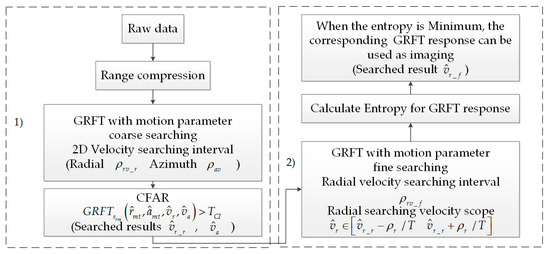
Figure 2.
Flowchart of the moving ship target detection and imaging.
Step 1: Coarse searching motion parameter for GRFT-based detection
After the range compression, the target’s 2D echoes are processing by (19) with the motion parameters’ coarse searching interval. Motion parameters’ searching interval is obtained by (23) and (24) in Section 3.3.2. The radial and azimuth velocity searching scope are and , respectively. When the searching velocities have satisfied the focusing requirement (both and are shown in Section 3.3.1), the amplitude of GRFT response is greater than the CFAR detection threshold. From [48], the CFAR detection threshold can be obtained as
When the GRFT response is greater than threshold, the radial and the azimuth searched velocity are and , respectively. Unfortunately, due to the accuracy of the radial searched velocity is not enough, the azimuth shift occurs in GRFT response. So, it is necessary to relocate the moving ship target in imaging.
Step 2: Fine searching motion parameter for GRFT-based imaging
Using GRFT to realize the moving ship target imaging with fine searching motion parameter, the radial velocity’s searching interval is given by (25) in Section 3.3.2; the radial velocity’s searching scope is ; and, the azimuth searching velocity is set as . The minimum entropy (26), which has obtained by Section 3.4, is used as criterion to determine whether the relocation requirement ( is shown in Section 3.3.1) is satisfied. When the entropy of GRFT response is minimum, the radial searched velocity is . The GRFT response to and can be used as the moving ship target’s image.
3.2. GRFT-Based Signal Integration
The schematic diagram of GRFT-based signal integration is given in Figure 3. Generally, the echo of moving target has cross range cell migration. When the signal has been submerged in the noise, the traditional integration method, such as MTD, which integrates just in a range unit, cannot be used. From Figure 3, the echoes after range compression are distributed in multiple range units that can be described by . GRFT use (19) to integrate signal by searching , , , . That is, represents the signal in at slow time and is used to compensate phase fluctuation. At the same time, the integral realize the signal integration in whole . Since is close enough to , the signal will be integrated in the corresponding range and azimuth position searching grid, such as and , where the moving target located in ACM. Therefore, GRFT can realize coherent integration in , which makes it superior than the traditional integration method.
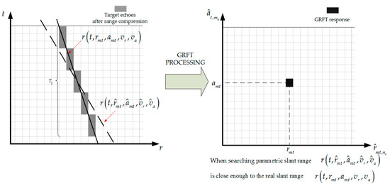
Figure 3.
The schematic diagram of generalized Radon-Fourier transform (GRFT)-based signal integration.
The GRFT-based signal integration processing for moving ship targets is given, as follows: (1) Determine range-azimuth 2D position and radial-azimuth 2D velocity searching grid according to requirements of the resolution and GRFT responses to different motion parameters. (2) Based on 2D position and 2D velocity searching grid, signal integration can be realized by (19). (3) Each of 2D velocity searching grid produces a GRFT response, which is the integration gain in 2D position searching grid.
There are two key issues in signal integration processing, as follows. Firstly, the 2D position searching grid is divided based on resolution. According to the SAR principle [1], the range and the azimuth resolution are and , respectively. The position of moving targets at ACM just needs to be located in the resolution cell. Therefore, the range position searching grid is and the azimuth position searching grid is .
Secondly, 2D velocity searching grid needs to be divided. The radial and azimuth velocity searching scope are and , respectively. Unfortunately, the 2D velocity searching grid dividing requires the searching interval. Therefore, the GRFT response to different motion parameters must be studied to obtain 2D velocity searching interval.
3.3. Influence of Different Motion Parameters on Signal Integration
3.3.1. GRFT Response to Different Searching Motion Parameters
In GRFT, the parameters’ searching interval is very important. When the parameters’ searching interval is too large, GRFT cannot be focused, leading to detection failure [49]. On the contrary, the calculation is too huge. Therefore, the GRFT response to different searching parameters needs to be studied.
Since the searching parameters, such as , , , and are different with the motion parameters, there are several kinds of GRFT response, such as moving targets completely focused, azimuth shift, completely unfocused, and azimuth defocused. According to (21), three different cases that are based on different radial and azimuth searching velocity are analyzed in Appendix C.
The analysis results can be given, as following. Since , the GRFT response will be approximately zero. Since both radial and azimuth velocity are searched inaccurately, the azimuth shift and the azimuth defocus in GRFT response equal to and , respectively. In this case, since and , the GRFT response of moving target is located accurately and the azimuth defocus is equal to . When and , the GRFT response of the moving target is focused and the azimuth shift equals to . Since the 2D velocity is searched accurately, the moving target can be completely focused where it is located at ACM. The GRFT response to different searching motion parameter can be summarized in Table 2.
Table 2.
GRFT responses to different searching motion parameters.
3.3.2. Motion Parameters’ Searching Interval
Unfortunately, only the completely focused requirements are used as the searching interval, resulting in the searching computation is too large. From Table 2, when the 2D searching velocity does not satisfy or , the GRFT response will become completely unfocused or azimuth defocused, which leads to its amplitude decrease. Due to the constant false-alarm rate (CFAR) detection being sensitive to signal SNR, it can be used to determine whether the 2D searching velocity satisfies above requirements.
The moving ship target relocation is also an important task of ship surveillance. Therefore, the accuracy of motion parameters needs to satisfy not only the focusing requirements ( and ), but also the relocation requirements (). According to , the coarse and the fine searching interval are proposed to satisfy the focusing and the relocation requirements, respectively. In this case, the computation of the GRFT processing can be greatly reduced. Two kinds of motion parameters’ searching interval are presented, as follows.
1. Motion parameters’ coarse searching interval
(1) Radial velocity’s coarse searching interval
Form Table 2, since is not satisfied, the GRFT response will be approximately zero. The radial velocity’s coarse searching interval can be expressed as
(2) Azimuth velocity searching interval
When , the target is defocused along azimuth direction and the azimuth defocus equals to . Therefore, the azimuth velocity searching interval can be expressed as
The 2D velocity searching grid is divided by (23) and (24), and then the moving target signal is integrated using (19). When the 2D searching velocity satisfies both and , the moving targets are focused without azimuth defocus, which can realize target detection. At this time, the radial and azimuth searching velocity of GRFT are the motion parameters searched value in coarse searching.
However, since is not satisfied, the azimuth shift appears in the GRFT response. Note that the relative position between the static targets is not changed, that is the static targets have the same azimuth shift. Unfortunately, the azimuth shift, which is related to the motion between targets and platform, is not the same between the static and the moving targets. Therefore, the moving targets imaging needs relocation and a fine searching of the radial velocity is required.
2. Motion parameters’ fine searching interval
When is not satisfied, the GRFT response is shifted along the azimuth. Consequently, the radial velocity’s fine searching interval can be obtained as
GRFT is a kind of FBD-based methods, that is the GRFT response can be used as the imaging of moving ship targets, since and . is satisfied by coarse-searched motion parameter. Unfortunately, the radial velocity’s fine searching will obtain multiple GRFT responses for a moving target, resulting in CFAR criteria that cannot be used to determine whether the searching velocity satisfies . At the same time, the ship target is a kind of extended target that cannot be estimated by finding the maximum value within a resolution cell. Therefore, in Section 3.4, the minimum entropy will be used as the criterion to realize moving targets imaging.
3.4. Imaging Based on the Minimum Entropy
The imaging of moving ship targets need to satisfy both focusing and relocation requirements. However, CFAR criterion cannot determine whether the relocation requirement is satisfied, that is, other kind of criterion is required to the motion parameters’ fine searching.
The entropy is a measure of energy divergence [50]. It is well known that when the motion searching parameter is closer to the true value, the signal integration is focused better and the entropy is smaller. Thus, the minimum entropy can be the criterion to determine whether the radial searching velocity is closest to the true velocity. From (21), the minimum entropy for GRFT can be obtained as
where , is the azimuth searched velocity obtained by the coarse-searched motion parameters. Because the entropy calculates the energy integration in the region of interest, the motion parameters estimation of the extended targets can be realized and the moving ship target can be relocated in imaging.
4. Numerical Experiments and Performance Analysis
In this section, numerical experiments are carried out to verify the effectiveness of the proposed GRFT-based detection and imaging methods for moving ship targets in GEO SAR. In Section 4.1, the GRFT responses is verified, which proposed in Section 3.3. Subsequently, the 2D raw echoes of a moving ship target are generated in apogee of GEO SAR to verify the detection and imaging methods that are proposed by Section 3.1. In Section 4.2, the GRFT-based moving ship targets detection is obtained. In Section 4.3, the GRFT-based imaging with the minimum entropy and evaluation of imaging are given. The system parameters of GEO SAR for the simulation are given as Table 3.
Table 3.
GEO SAR system parameters.
4.1. GRFT Responses
In Section 3.3, GRFT responses to different searching motion parameters are analyzed. In this section, the simulation is obtained to verify the validity of GRFT responses.
Suppose that GEO SAR is near apogee; the moving ship target is located in the center of the scene at ACM; the radial velocity is m/s; and, the azimuth velocity is m/s. In order to analyze the experimental results easily, the ship target is represented by the point target. The GRFT responses to three kinds of motion parameters’ searching interval are simulated, as follows.
(1) GRFT response to radial velocity’s coarse searching
According to (23), the radial velocity’s coarse searching grid can be divided as (m/s); the azimuth searching velocity is set as m/s. The GRFT response can be obtained by (19). The simulation results are shown in Figure 4.
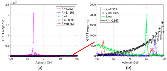
Figure 4.
Azimuth profile of GRFT responses to radial velocity’s coarse searching: (a) all coarse-searched radial velocities (the pink line represents ); (b) enlarged view of GRFT response when .
The azimuth profile of GRFT responses with radial velocity’s coarse searching is shown in Figure 4. The azimuth profile of GRFT responses with all coarse-searched radial velocities are shown in Figure 4a. When is satisfied, the GRFT response is much larger than other search velocities. When the radial searching velocities do not satisfy , the enlarged view of GRFT responses are shown in Figure 4b.
From the simulation results, it can be seen that the moving ship target can be focused in an azimuth resolution cell, since . Otherwise, the GRFT response is very weak.
(2) GRFT response to radial velocity’s fine searching
Since is not satisfied, the GRFT response is shifted along azimuth and the azimuth shift equal to . Based on (25), the radial velocity’s fine searching grid can be set as (m/s), ; the azimuth searching velocity is set as m/s. The GRFT responses to the radial velocity’s fine searching are shown in Figure 5.
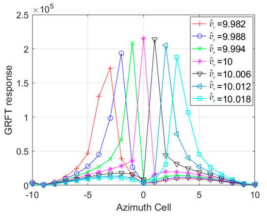
Figure 5.
Azimuth profile of GRFT responses to radial velocity’s fine searching.
It can be seen from simulation results that since ( m/s) the moving ship targets is located accurately. On the contrary, the azimuth shift equal to .
(3) GRFT response to azimuth velocity’s searching
Since , the GRFT response of moving ship targets do not defocus along azimuth. Otherwise, the azimuth defocus is equal to . Based on (24), the azimuth velocity searching grid can be divided as (m/s), ; the radial searching velocity is set as m/s. The simulation results are shown in Figure 6.
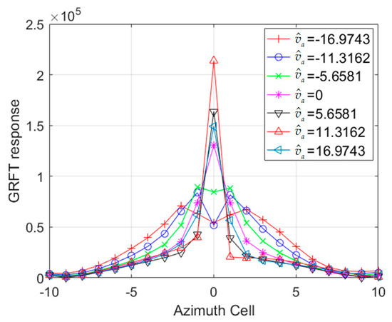
Figure 6.
Azimuth profile of GRFT responses to azimuth velocity searching.
From Figure 6, since ( m/s), the target is focused in a resolution cell and . When is not satisfied, the amplitude of the GRFT response is decreased due to being partially focused. The azimuth defocus is equal to .
The above three cases are verified the GRFT response to radial velocity’s coarse searching, fine searching, and azimuth velocity’s searching, respectively. Accordingly, the simulation results are consistent with the theoretical analysis results that are shown in Table 2.
4.2. Simulation Results of the GRFT-Based Detection
The moving ship target is represented by five point targets and is located in the center of the scene at ACM; the radial velocity is m/s; and, the azimuth velocity is m/s. We generate the echoes of the moving ship target (a target with five points) into the background raw data of GEO SAR. After the range compression, the received signal of moving ship target is completely submerged in the noise. The simulation results are shown in Figure 7.
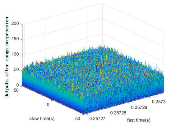
Figure 7.
Outputs of signal data after the range compression.
The range of the radial and the azimuth searching velocity is ; where m/s due to the maximum velocity of the ship is 33 knots (about 16.98 m/s); the 2D searching velocity grid is divided according to (23) and (24). The GRFT response with coarse-searched motion parameters is simulated by (19). When the 2D searching parameters are equal to m/s and m/s, the corresponding GRFT response is greater than (22). The corresponding GRFT response is shown as Figure 8. The ‘red cross’ in the center of scene represents the location of target at ACM. From simulation results, although the accuracy of 2D searched velocity satisfy the focusing requirement, the GRFT response cannot be used as the imaging of moving ship targets due to the azimuth shift. Therefore, it is necessary to relocate the target.
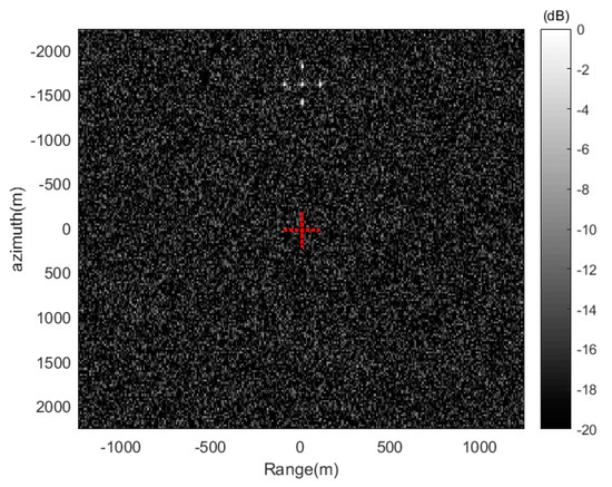
Figure 8.
The corresponding GRFT response for target detection.
Due to the orbital height of GEO SAR varies with the orbital position, we set the scope of slant range () in all orbit positions as 33,000 km–40,000 km. From [35], the signal SNR after range compression can be given as
where is Boltzmann constant and is receiver temperature. Therefore, the corresponding scope of is dB– dB. After signal integration by GRFT, the SNR of GRFT response will become dB– dB and dB– dB, since the integration times are equal to 10 s and 100 s, respectively.
In order to prove the superiority of proposed integration method in GEO SAR, MTD, and Radon transform (RT) are used as comparisons that can be seem as the typical method of short-time integration and long-time incoherent integration, respectively. After signal integration by RT, the SNR of output will become dB– dB and dB– dB, since the integration time equal to 10 s and 100 s, respectively. After processing by MTD with any integration time, the MTD output has been submerged in noise.
Furthermore, the detection probability of MTD, RT and GRFT can be calculated with a given constant false alarm ratio , which are shown as Figure 9. From the simulation results, when the integration time equal to 10 s, the GRFT can obtain detection probability more than around km and the other two methods cannot be used in target detection. When the integration time equal to 100 s, the GRFT can realize high performance detection in any orbital position. At the same time, RT can realize detection around km and MTD cannot realize detection. Because MTD can integrate signal in just in a single range unit, it cannot realize detection in GEO SAR. Although RT realizes signal integration across range unit, it does not compensate phase fluctuation. Therefore, GRFT is superior to RT and MTD in GEO SAR.
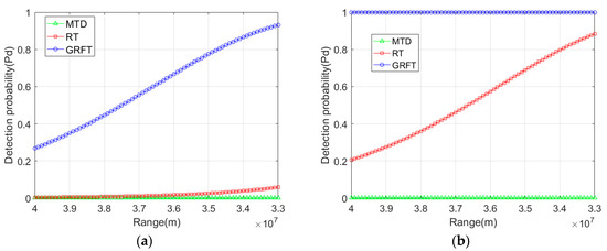
Figure 9.
The detection probability for different integration methods: (a) when integration time equals to 10 s; and, (b) when integration time equals to 100 s.
4.3. Simulation Results of the GRFT-Based Imaging
The GRFT-based imaging with fine-searched motion parameters is processed after the detection. Where the range of fine-searched radial velocity is (m/s); the radial searching velocity grid is divided by (25); and, the azimuth searching velocity is m/s. The entropy of the GRFT response to fine-searched motion parameters can be simulated by (26) and the simulation results are shown as Figure 10a. Since m/s, the entropy of GRFT response is minimum and the corresponding GRFT response is shown as Figure 10b. It can be seen from Figure 10b that, since the entropy of GRFT response is minimum, the accuracy of radial searched velocity can realize the moving ship target relocation, which satisfy . The parameters of the moving ship target are summarized in Table 4. Meanwhile, the evaluation of each point targets in corresponding GRFT response are given in Table 5. Figure 11 is obtained PSLR of point target imaging in range and azimuth directions.
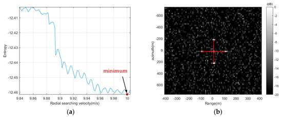
Figure 10.
The simulation results for fine-searched motion parameters: (a) The entropy for GRFT response to fine-searched radial velocity; and, (b) The corresponding GRFT response when the entropy is minimum.
Table 4.
The parameters of the moving ship target.
Table 5.
Evaluation of GRFT-based point target imaging.
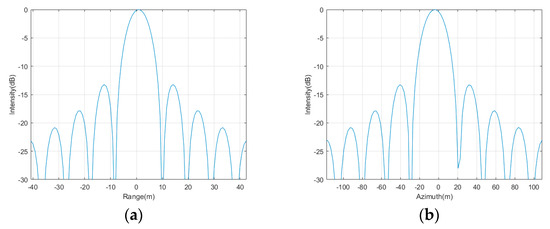
Figure 11.
Range profile and azimuth profile of GRFT-based point target imaging: (a) the range profile; and, (b) the azimuth profile.
To verify the necessity of minimum entropy, we set the radial searching velocity as (m/s), . The corresponding GRFT responses and azimuth profiles are shown in Figure 12. From the simulation results, since the radial searching velocity do not satisfy the relocation requirement, the azimuth shift is obtained and the PSLR of GRFT response is not much different. Therefore, due to the entropy simulation results in this section, the minimum entropy can realize the relocation of the moving ship target, which can be used as the criterion of the GRFT-based imaging.
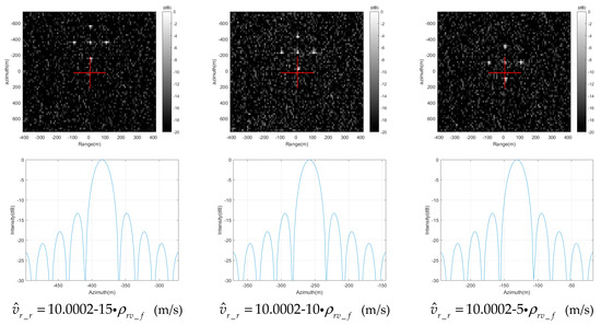
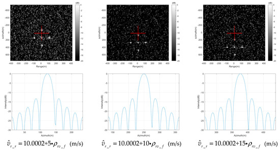
Figure 12.
GRFT responses and azimuth profiles to different fine-searched radial velocities.
5. Conclusions
Due to short revisiting time and large wide coverage, GEO SAR has a greater researching value than other platforms in the moving ship target surveillance. However, some problems have not been resolved, such as invalid traditional range model and weak signal echo. In this paper, the proposed accurate slant range has considered the characteristics of curved trajectory and non-negligible signal round-trip delay; the redefined GRFT model has resolved the problem of moving ship targets’ signal integration in GEO SAR; the proposed processing realize detection, relocation, and imaging of the moving ship target.
In order to solve the problems of the moving ship target detection and imaging in GEO SAR. Firstly, from the analysis results, only the influence of approximately uniform moving ship target velocity on first-order and second-order coefficients cannot be negligible, and then the accurate slant range with four-order coefficients is given. Secondly, the GRFT model is redefined for moving ship targets. For the sake of realizing the signal integration, GRFT responses, such as completely unfocused, azimuth defocused, azimuth shift, and completely focused are analyzed. Resulting in two kinds of motion parameters’ searching interval, such as coarse and fine searching interval, are given to realize the focusing (overcoming completely unfocused and azimuth defocused) and relocation (overcoming azimuth shift and realizing completely focused) of moving ship targets in the GRFT response, respectively. Because GRFT is a kind of the FBD method, when both focusing and relocation requirement are satisfied, the corresponding GRFT response can be used for the imaging of moving targets. Thirdly, the processing of detection and imaging is proposed. It can be summarized as the detection with coarse-searched parameters and imaging with fine-searched parameters which satisfy requirements of focusing and relocation, respectively.
Finally, numerical experiments and scene simulations are provided to demonstrate the effectiveness of the proposed methods in GEO SAR with 53° orbit inclination. From the simulation results, the proposed method can realize the moving ship targets imaging with azimuth PSLR and ISLR of about −13.27 dB and −9.77 dB, respectively. At the same time, the proposed imaging method can satisfy the relocation requirement, resulting in the moving ship target can be accurately located in an azimuth resolution cell of SAR imaging.
Author Contributions
Y.Z. and X.D. conceived and designed the method; W.X. and C.H. guided the students to complete the research; Y.S. performed the simulation and experiment test; Y.Z. and X.D. wrote the paper.
Funding
This work was supported in part by the National Natural Science Foundation of China under Grant Nos. 61501032, 61471038, 61427802, the Chang Jiang Scholars Program (T2012122), and in part by the 111 project of China under Grant B14010, the Beijing Natural Science Foundation under Grant 4162052.
Acknowledgments
The authors would like to thank all reviewers and editors for their comments on this paper.
Conflicts of Interest
The authors declare no conflict of interest.
Appendix A. Coefficients in Equation (2)
The zero-order to fourth-order coefficients of the Taylor series expansion in the slant range can be expressed as
The zero-order to third-order coefficients of Taylor series expansion in the relative motion between GEO SAR and the target within signal round-trip delay can be expressed as
Appendix B. Influence of the Moving Ship Target Velocity on Slant Range
The slant range of moving ship targets is different from the static targets, resulting in the coefficients of (2) are not same with the static targets. Furthermore, the influence of the moving ship target velocity on each order coefficients is also different, so it is necessary to analyze the influence respectively.
Appendix B.1. Influence on and
The influence of the moving ship target velocity on the and in slant range is analyzed in this section. The influence on in (A4) can be defined as
Because of , (A10) can be approximated as
According to the above analysis, can be negligible. We set as resultant velocity with both radial and azimuth velocity equal to 20 m/s. The simulation results of (A10) based on Table 3 is shown in Figure A1.

Figure A1.
The influence of Target Motion on of slant range.
From Figure A1, it can be seen that is far less than , resulting in it can be negligible. Then The influence on in (A5) can be defined as
where and are first-order and second-order coefficients in slant range of the static target, respectively.
Because of , (A12) can be approximated as
Since and is far less than , (A15) can be negligible. The simulation results is shown as Figure A2. is far less than , that is the influence can be negligible.

Figure A2.
The influence of target motion on of slant range.
Appendix B.2. Influence on the Relative Motion between GEO SAR and the Target within Signal Round-Trip Delay
The influence of moving ship target motion on the relative motion between GEO SAR and the target within signal round-trip delay in (1) can be shown as
The influence on each order coefficients in (A6)–(A9) can be obtained as
Due to the norm calculation formula, (A18) can be obtained as
Based on Cauchy-Schwarz inequality, (A17), (A19) and (A20) can be given as
We set the velocity of the target as m/s. Using the parameters shown in Table 3, the maximum values of , and in all orbital positions are m, m/s2 and m/s3 which are known from STK software, respectively. So m, m/s, m/s2 and m/s3.
At present, the optimally range resolution in GEO SAR is 5 m. is constant and must be smaller than the range resolution, so there has no compensation needed. When the error caused by first-order coefficient is less than , the moving target do not produce the azimuth shift in focusing. That is, when integration time is less than s, is negligible. When , the error of second-order coefficient do not influence the moving target focusing. That is, when integration time is less than s, is negligible. Similarly, when the cubic phase error is less than , the error of third-order coefficient do not influence the moving target focusing. So when integration time is less than s, is negligible. The maximum integration time of GEO SAR with parameters shown in Table 3 is 300 s.
The simulation results of (A16) are shown as Figure A3. From the analysis and experimental results, it can be seen that the influence of moving ship target motion on the relative motion can be approximated as a constant and do not need compensation.
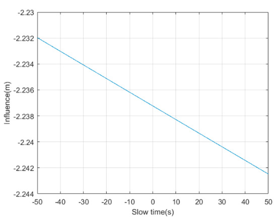
Figure A3.
The influence of target motion on the relative motion caused by signal round-trip delay.
The following conclusions can be obtained through analysis and simulation.
- The influence of the moving ship target velocity on and can be negligible.
- The influence of the moving ship target velocity on the relative motion caused by signal round-trip delay can be approximated as a constant and do not need compensation.
Appendix C. GRFT Response to Different Searching Motion Parameters
According to (21), three different cases based on different radial and azimuth searching velocity are discussed as follows
Case 1: when and , the moving target is completely focused
where the searching slant range of the moving ship target at the ACM is . From (A25), since the 2D velocity is searched accurately, the target is completely focused within the 2D position grid where it is located at ACM.
Case 2: When , and , the moving target is shifted in azimuth or completely unfocused
where the approximation in (A26) is obtained according to . There have two cases of radial searching velocity as follows
(a) If , (A26) can be rewritten as
Because of the azimuth resolution equals to , (A27) can be rewritten as
After GRFT processing, the azimuth shift of moving targets is and then (A28) can be rewritten as
(A29) can be approximately understood as GRFT response is completely focused and accurately positioned since (). Otherwise, the position of the target is shifted along the azimuth and the azimuth shift equals to (). At the same time, the amplitude of GRFT response is reduced.
(b) If , (A26) can be rewritten as
The approximation holds when . In this case, the amplitude of GRFT response is too low, which causes the response to be submerged in noise.
Case 3: When , and , the moving target is defocused in azimuth
Based on the principle of stationary phase (PSP), (A31) can be approximated as
where , , and . The function in (A32) can be given as
where the cell number of azimuth defocus is . The azimuth defocus can be approximated as
The approximation holds since . When is satisfied, the moving target can be focused in an azimuth cell and the quadratic phase error (QPE) as follow
Therefore, when , the GRFT response of moving target is defocused along azimuth and the azimuth defocus equal to .
References
- Curlander, J.C.; Mcdonough, R.N. Synthetic Aperture Radar: Systems and Signal Processing; John Wiley & Sons: Hoboken, NJ, USA, 1991; pp. 3–7. [Google Scholar]
- Brusch, S.; Lehner, S.; Fritz, T.; Soccorsi, M.; Soloviev, A.; Schie, B.V. Ship surveillance with terrasar-x. IEEE Trans. Geosci. Remote Sens. 2011, 49, 1092–1103. [Google Scholar] [CrossRef]
- Song, S.; Xu, B.; Yang, J. Ship Detection in Polarimetric SAR Images via Variational Bayesian Inference. IEEE J. Sel. Top. Appl. Earth Observ. Remote Sens. 2017, 10, 2819–2829. [Google Scholar] [CrossRef]
- Wang, X.; Chen, C. Ship detection for complex background sar images based on a multiscale variance weighted image entropy method. IEEE Geosci. Remote Sens. Lett. 2017, 14, 184–187. [Google Scholar] [CrossRef]
- Iervolino, P.; Guida, R. A Novel Ship Detector Based on the Generalized-Likelihood Ratio Test for SAR Imagery. IEEE J. Sel. Top. Appl. Earth Observ. Remote Sens. 2017, 10, 3616–3630. [Google Scholar] [CrossRef]
- Ao, W.; Xu, F.; Li, Y.; Wang, H. Detection and Discrimination of Ship Targets in Complex Background From Spaceborne ALOS-2 SAR Images. IEEE J. Sel. Top. Appl. Earth Observ. Remote Sens. 2018, 11, 536–550. [Google Scholar] [CrossRef]
- Jansen, R.W.; Raj, R.G.; Rosenberg, L.; Sletten, M.A. Practical multichannel sar imaging in the maritime environment. IEEE Trans. Geosci. Remote Sens. 2018, 56, 4025–4036. [Google Scholar] [CrossRef]
- Martorella, M.; Pastina, D.; Berizzi, F.; Lombardo, P. Spaceborne radar imaging of maritime moving targets with the cosmo-skymed sar system. IEEE J. Sel. Top. Appl. Earth Observ. Remote Sens. 2014, 7, 2797–2810. [Google Scholar] [CrossRef]
- Pelich, R.; Longépé, N.; Mercier, G.; Hajduch, G.; Garello, R. Vessel refocusing and velocity estimation on sar imagery using the fractional fourier transform. IEEE Trans. Geosci. Remote Sens. 2016, 54, 1670–1684. [Google Scholar] [CrossRef]
- Weihing, D.; Suchandt, S.; Hinz, S.; Runge, H.; Bamler, R. Traffic parameter estimation using terrasar-x data. Int. Arch. Photogramm. Remote Sens. Spat. Inf. Sci. 2008, 37, 153–156. [Google Scholar]
- Livingstone, C.E.; Sikaneta, I.; Gierull, C.; Chiu, S.; Beaulne, P. Radarsat-2 System and Mode Description; Defence Research and Development Canada Ottawa: Ottawa, ON, Canada, 2006.
- Rousseau, L.P.; Gierull, C.; Chouinard, J.Y. First results from an experimental scansar-gmti mode on radarsat-2. IEEE J. Sel. Top. Appl. Earth Observ. Remote Sens. 2017, 8, 5068–5080. [Google Scholar] [CrossRef]
- Tomiyasu, K. Tutorial review of synthetic-aperture radar (sar) with applications to imaging of the ocean surface. Proc. IEEE 1978, 66, 563–583. [Google Scholar] [CrossRef]
- Madsen, S.N.; Edelstein, W.; Didomenico, L.D.; Labrecque, J. In A geosynchronous synthetic aperture radar; for tectonic mapping, disaster management and measurements of vegetation and soil moisture. In Proceedings of the IEEE 2001 International Geoscience and Remote Sensing Symposium, IGARSS ‘01, Sydney, Australia, 9–13 July 2002; Volume 441, pp. 447–449. [Google Scholar]
- Bruno, D.; Hobbs, S.E. Radar imaging from geosynchronous orbit: Temporal decorrelation aspects. IEEE Trans. Geosci. Remote Sens. 2010, 48, 2924–2929. [Google Scholar] [CrossRef]
- Ruiz-Rodon, J.; Broquetas, A.; Makhoul, E.; Guarnieri, A.M.; Rocca, F. Nearly zero inclination geosynchronous sar mission analysis with long integration time for earth observation. IEEE Trans. Geosci. Remote Sens. 2014, 52, 6379–6391. [Google Scholar] [CrossRef]
- Hobbs, S.; Mitchell, C.; Forte, B.; Holley, R.; Snapir, B.; Whittaker, P. System design for geosynchronous synthetic aperture radar missions. IEEE Trans. Geosci. Remote Sens. 2014, 52, 7750–7763. [Google Scholar] [CrossRef]
- Bruno, D.; Hobbs, S.E.; Ottavianelli, G. Geosynchronous synthetic aperture radar: Concept design, properties and possible applications. Acta Astronaut. 2006, 59, 149–156. [Google Scholar] [CrossRef]
- Zheng, W.; Hu, J.; Zhang, W.; Yang, C.; Li, Z.; Zhu, J. Potential of geosynchronous sar interferometric measurements in estimating three-dimensional surface displacements. Sci. China (Inf. Sci.) 2017, 60, 060304. [Google Scholar] [CrossRef]
- Li, Y.; Monti Guarnieri, A.; Hu, C.; Rocca, F. Performance and requirements of geo sar systems in the presence of radio frequency interferences. Remote Sens. 2018, 10, 82. [Google Scholar] [CrossRef]
- Fuster, R.M.; Usón, M.F.; Ibars, A.B. Interferometric orbit determination for geostationary satellites. Sci. China (Inf. Sci.) 2017, 60, 060302. [Google Scholar] [CrossRef]
- Hu, C.; Long, T.; Zeng, T.; Liu, F.; Liu, Z. The accurate focusing and resolution analysis method in geosynchronous sar. IEEE Trans. Geosci. Remote Sens. 2011, 49, 3548–3563. [Google Scholar] [CrossRef]
- Ding, Z.; Shu, B.; Yin, W.; Zeng, T.; Long, T. A modified frequency domain algorithm based on optimal azimuth quadratic factor compensation for geosynchronous sar imaging. IEEE J. Sel. Top. Appl. Earth Observ. Remote Sens. 2016, 9, 1119–1131. [Google Scholar] [CrossRef]
- Sun, G.C.; Xing, M.; Wang, Y.; Yang, J.; Bao, Z. A 2-d space-variant chirp scaling algorithm based on the rcm equalization and subband synthesis to process geosynchronous sar data. IEEE Trans. Geosci. Remote Sens. 2014, 52, 4868–4880. [Google Scholar]
- Yin, W.; Ding, Z.; Xiaojun, L.U.; Zhu, Y. Beam scan mode analysis and design for geosynchronous sar. Sci. China (Inf. Sci.) 2017, 60, 060306. [Google Scholar] [CrossRef]
- Hu, C.; Li, Y.; Dong, X.; Wang, R.; Ao, D. Performance analysis of l-band geosynchronous sar imaging in the presence of ionospheric scintillation. IEEE Trans. Geosci. Remote Sens. 2016, 55, 159–172. [Google Scholar] [CrossRef]
- Hu, C.; Li, Y.; Dong, X.; Ao, D. Avoiding the ionospheric scintillation interference on geosynchronous sar by orbit optimization. IEEE Geosci. Remote Sens. Lett. 2016, 13, 1676–1680. [Google Scholar] [CrossRef]
- Dexin, L.I.; Rodriguez-Cassola, M.; Prats-Iraola, P.; Dong, Z.; Manqing, W.U.; Moreira, A. Modelling of tropospheric delays in geosynchronous synthetic aperture radar. Sci. China (Inf. Sci.) 2017, 60, 060307. [Google Scholar]
- Hu, C.; Li, Y.; Dong, X.; Long, T. Optimal data acquisition and height retrieval in repeat-track geosynchronous sar interferometry. Remote Sens. 2015, 7, 13367–13389. [Google Scholar] [CrossRef]
- Hu, C.; Li, Y.; Dong, X.; Wang, R.; Cui, C. Optimal 3d deformation measuring in inclined geosynchronous orbit sar differential interferometry. Sci. China (Inf. Sci.) 2017, 60, 060303. [Google Scholar] [CrossRef]
- Hu, C.; Li, Y.; Dong, X.; Cui, C.; Long, T. Impacts of temporal-spatial variant background ionosphere on repeat-track geo d-insar system. Remote Sens. 2016, 8, 916. [Google Scholar] [CrossRef]
- Hobbs, S.; Convenevole, C.; Guarnieri, A.M.; Wadge, G. In Geostare system performance assessment methodology. In Proceedings of the Geoscience and Remote Sensing Symposium, Beijing, China, 10–15 July 2016; pp. 1404–1407. [Google Scholar]
- Gao, G.; Ouyang, K.; Luo, Y.; Liang, S.; Zhou, S. Scheme of parameter estimation for generalized gamma distribution and its application to ship detection in sar images. IEEE Trans. Geosci. Remote Sens. 2017, 55, 1812–1832. [Google Scholar] [CrossRef]
- Stasolla, M.; Mallorqui, J.J.; Margarit, G.; Santamaria, C.; Walker, N. A comparative study of operational vessel detectors for maritime surveillance using satellite-borne synthetic aperture radar. IEEE J. Sel. Top. Appl. Earth Observ. Remote Sens. 2016, 9, 2687–2701. [Google Scholar] [CrossRef]
- Skolnik, M. Radar Handbook, 3rd ed.; McGraw-Hill Education: New York, NY, USA, 2008. [Google Scholar]
- Schleher, D.C. Mti and Pulsed Doppler Radar; Artech House Radar Library; Atrech House: Boston, MA, USA, 1991. [Google Scholar]
- Ringel, M.B.; Mooney, D.H.; Long, W.H., III. F-16 pulse doppler radar (an/apg-66) performance. IEEE Trans. Aerosp. Electr. Syst. 1983, AES-19, 147–158. [Google Scholar] [CrossRef]
- Xu, J.; Peng, Y.N.; Xia, X.G.; Farina, A. Focus-before-detection radar signal processing: Part I—Challenges and methods. IEEE Aerosp. Electr. Syst. Mag. 2017, 32, 48–59. [Google Scholar] [CrossRef]
- Chen, X.; Cai, F.; Cong, Y.; Guan, J. In Radon-fractional fourier transform and its application to radar maneuvering target detection. In Proceedings of the International Conference on Radar, Adelaide, Australia, 9–12 September 2013; pp. 346–350. [Google Scholar]
- Xu, J.; Zhou, X.; Qian, L.C.; Xia, X.G.; Long, T. Hybrid integration for highly maneuvering radar target detection based on generalized radon-fourier transform. IEEE Trans. Aerosp. Electr. Syst. 2017, 52, 2554–2561. [Google Scholar] [CrossRef]
- Chen, X.; Guan, J.; Liu, N.; He, Y. Maneuvering target detection via radon-fractional fourier transform-based long-time coherent integration. IEEE Trans. Signal Process. 2014, 62, 939–953. [Google Scholar] [CrossRef]
- Chen, X.; Guan, J.; He, Y.; Zhang, J. Detection of low observable moving target in sea clutter via fractal characteristics in fractional fourier transform domain. Iet Radar Sonar Navig. 2013, 7, 635–651. [Google Scholar] [CrossRef]
- Huang, P.; Liao, G.; Yang, Z.; Xia, X.G.; Ma, J.; Zheng, J. Ground maneuvering target imaging and high-order motion parameter estimation based on second-order keystone and generalized hough-haf transform. IEEE Trans. Geosci. Remote Sens. 2016, 55, 320–335. [Google Scholar] [CrossRef]
- Xu, J.; Xia, X.G.; Peng, S.B.; Yu, J.; Peng, Y.N.; Qian, L.C. Radar maneuvering target motion estimation based on generalized radon-fourier transform. IEEE Trans. Signal Process. 2012, 60, 6190–6201. [Google Scholar]
- Renga, A.; Moccia, A. Use of doppler parameters for ship velocity computation in sar images. IEEE Trans. Geosci. Remote Sens. 2016, 54, 3995–4011. [Google Scholar] [CrossRef]
- Sletten, M.A.; Rosenberg, L.; Menk, S.; Toporkov, J.V.; Jansen, R.W. Maritime signature correction with the nrl multichannel sar. IEEE Trans. Geosci. Remote Sens. 2016, 54, 6783–6790. [Google Scholar] [CrossRef]
- Hu, C.; Long, T.; Liu, Z.; Zeng, T.; Tian, Y. An improved frequency domain focusing method in geosynchronous sar. IEEE Trans. Geosci. Remote Sens. 2014, 52, 5514–5528. [Google Scholar]
- Richards, M.A. Threshold Detection of Radar Targets, IET Digital Library. Princ. Mod. Radar Basic Princ. 2010, 547–587. [Google Scholar] [CrossRef]
- Xu, J.; Yu, J.; Peng, Y.N.; Xia, X.G. Radon-fourier transform for radar target detection (ii): Blind speed sidelobe suppression. IEEE Trans. Aerosp. Electr. Syst. 2011, 47, 2473–2489. [Google Scholar] [CrossRef]
- Wang, R.; Zeng, T.; Hu, C.; Yang, J. Accurate range profile alignment method based on minimum entropy for inverse synthetic aperture radar image formation. Iet Radar Sonar Navig. 2016, 10, 663–671. [Google Scholar] [CrossRef]
© 2018 by the authors. Licensee MDPI, Basel, Switzerland. This article is an open access article distributed under the terms and conditions of the Creative Commons Attribution (CC BY) license (http://creativecommons.org/licenses/by/4.0/).