Ocean Backscatter Profiling Using High-Spectral-Resolution Lidar and a Perturbation Retrieval

Abstract

Ocean lidar attenuation and scattering parameters were derived from a high-spectral-resolution lidar (HSRL) using two different retrieval techniques. The first used the standard HSRL retrieval, and the second used only the total backscatter channel and a perturbation retrieval (PR). The motivation is to evaluate differences between the two techniques that would affect the decision of whether to use a simple backscatter lidar or a more complex HSRL in future applications. For the data set investigated, the attenuation coefficient from the PR was an average of 11% lower than that from the HSRL. The PR estimate of the scattering parameter decreased with depth relative to the HSRL estimate, although the overall bias was zero as a result of the calibration procedure. Near the surface, the coefficient of variability in both estimates of attenuation and in HSRL estimates of scattering were around 5%, but that in the PR estimate of scattering was over 10%. At greater depths, the variability increases for all of the profile parameters. The correlation between the two estimates of attenuation coefficient was 0.7. The correlation between scattering parameters was > 0.8 near the surface, but decreased to 0.4 at a depth of around 20 m. Overall, the PR performed better relative to the HSRL in offshore waters than in nearshore waters.

1. Introduction

Two different lidar configurations have been used to obtain profiles of optical properties of the upper ocean from aircraft [1]. The earliest measurements used a simple polarized backscatter lidar [2,3,4]. This configuration has the advantage of simplicity and lower cost, but an inversion must be applied to the data to infer two quantities from a single measurement. In addition, obtaining quantitative information on scattering requires absolute radiometric calibration of the system. More recently, the High Spectral Resolution Lidar (HSRL) configuration, originally developed for atmospheric applications [5,6], has been used in the ocean [7,8,9,10]. This configuration is more advanced and complex, but provides an additional piece of information to the inversion, and importantly does not require absolute calibration.

In its simplest form, the signal from a single channel of a profiling lidar can be expressed as [11]

$$S\left(z\right)=AT\beta \left(\mathsf{\pi },z\right)\exp \left[-2{\displaystyle \underset{0}{\overset{z}{\int }}d{z}^{\prime }}\alpha \left(z^{\prime }\right)\right],$$

(1)

where z is measurement depth, z′ is a depth variable for integration, A is a calibration factor that includes system parameters and measurement geometry, T is the atmospheric transmission from the aircraft to the sea surface and back, β(π,z) is the volume scattering function for both seawater and hydrosols at the lidar scattering angle of π radians, and α(z) is the lidar attenuation coefficient. The range-squared loss between the aircraft and the sea surface is assumed to be included in the calibration factor. The additional range-squared loss in the water is negligible, because the maximum propagation distance in water is much smaller than the range in air. The objective is to measure the profiles β(π,z) and α(z), and these are the two quantities mentioned in the previous paragraph. For typical airborne lidar geometries, α is nearly equal to the diffuse attenuation coefficient, K_d, and β can be used to estimate the particulate contribution to the backscattering coefficient, b_bp [7,12]. These parameters are important because of the information they can provide about the biogeochemistry of the ocean.

For the backscatter lidar, some method must be found to derive both β(π,z) and α(z) from a single signal. There are several approaches available, depending on the ocean optical conditions. If the water column is well mixed, both α and β will be constant over the profile. In this case, α can be found from the slope of the logarithm of the signal and this can be used to estimate β. If the type of particles in the water does not change with depth, the profile of the optical properties will depend only on the profile of the number density of those particles. In this case, the lidar ratio (α_p/β_p, where the subscript p refers to the values after subtracting the contribution from pure seawater) of those particles can be used, along with the known values for seawater, to resolve the ambiguity [13]. If changes in the depth profile of the optical properties are not too extreme, they can be represented by the sum of their depth-averaged values and a depth-dependent perturbation. In this case, the integral of the perturbation of the attenuation will be small and can be neglected. With this approximation, the depth profile of the scattering can be found [14]. That study showed that β(z) could be determined to within about 10% for thin plankton layers, assuming that the lidar profile was accurately calibrated against satellite-based chlorophyll estimates.

For HSRL, an additional receiver channel removes the backscattered light from particulate scattering by spectral filtering [15]. Since the volume scattering function from seawater is known [16], this channel provides the profile of α directly. Independently, the ratio of the two channels provides the profile of β. A further advantage of HSRL is that absolute calibration is not necessary as long as the relative calibration of the two channels is known. The calibration of the relative gain between the channel is performed during each flight and has been assessed to be stable within a few percent [17].

In this paper, we directly compared backscatter and HSRL techniques. Data from an HSRL were processed with the standard HSRL method that uses the information in the additional, filtered channel. In addition, a perturbation retrieval (PR) was applied to the primary seawater-plus-particulate channel, and the results were compared.

2. Materials and Methods

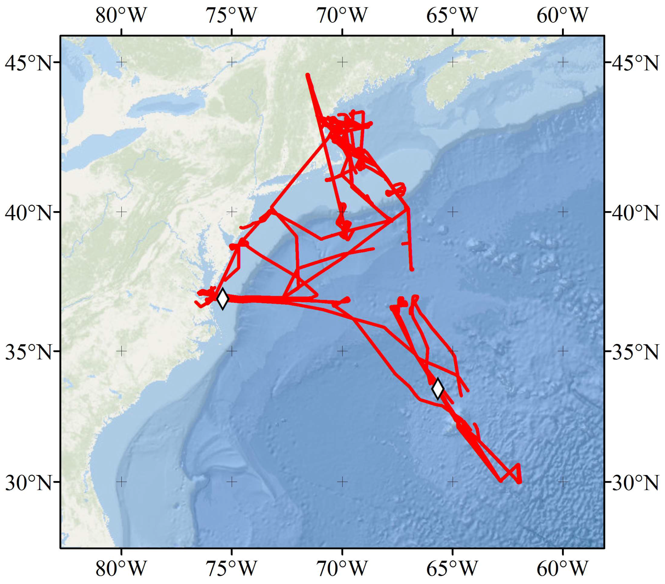
The data used in this study were collected using the NASA HSRL-1 during the Ship-Aircraft Bio-Optical Research Experiment (SABOR). SABOR took place in the NW Atlantic Ocean (Figure 1) between 18 July and 5 August 2014, covering both open ocean and coastal regions. The flights were made at a nominal altitude of 9000 m and speed of 100 m s⁻¹. The lidar has been described in previous publications [9,17], but the salient features are repeated here.

The laser produced linearly polarized light at 1064 nm and 532 nm, but only the latter is used for profiling of the ocean. The pulse repetition rate is 4 kHz, the pulse width is 6 ns, and the pulse energy is 2.5 mJ. The transmitted beam divergence is 0.8 mrad, which produces a spot diameter of about 7 m on the surface from the normal flight altitude of 9000 m. The laser light has a narrow frequency spectrum (~50 MHz) with a center frequency that is locked to the center of an iodine absorption line.

The receiver used a 40 cm diameter telescope with a 1 mrad field of view. The 532 nm light was then split into three channels—one for light that is co-polarized with the transmitter, one for light that is cross-polarized with respect to the transmitter, and one for co-polarized light that is filtered to pass only the frequency-shifted Brillouin component. The latter was accomplished with an iodine filter that only passes light that has been Doppler shifted by 7–9 GHz by Brillouin scattering. The transmission of unshifted light by this filter was <10⁻⁵, and the fraction of laser light in the filter passband was about 3 × 10⁻⁴. Each of the three channels is independently detected using a photomultiplier tube (PMT) and a hybrid photodetector (HPD) that combines a photocathode with an avalanche diode for photoelectron multiplication. Roughly 55% of the incoming light was directed toward the PMTs and 45% to the HPDs. Each of the resulting six signals is digitized at 120 MHz and averaged for 2000 pulses to produce each recorded profile. The 120 MHz sample rate produces a depth resolution of 0.9 m in water. The pulse averaging produces a horizontal resolution of about 50 m.

Several quality control filters were applied to the profiles. Valid ocean profiles could not be obtained when there were clouds between the aircraft and the surface. These shots were identified by a surface return in the HPD Brillouin channel below 1000 digitization levels, and removed from the analysis. Also, profiles were occasionally affected by a rapid change in the surface position during the 0.5 s averaging periods. These were removed by requiring that the full width at half maximum of the ocean surface return be five samples (4.7 m) or less.

The sea surface in each profile was identified as the sample where the HPD Brillouin return was maximum. The other signals were then shifted to align with this signal. The depth penetration for each profile was defined as the depth at which either the attenuated Brillouin signal or the attenuated co-polarized signal dropped below a threshold value. For each profile, the threshold was calculated from the deepest 100 samples in the profile, for which the ocean scattering signal is negligible due to attenuation. Specifically, the threshold for each channel was calculated as five standard deviations of those 100 samples above their mean value.

The profile of the co-polarized component of the total (seawater and particulate) volume scattering function, β, at the lidar scattering angle of 180° was calculated using two different techniques. Hereafter, we will refer to this quantity as the volume backscattering, and drop the explicit dependence on the scattering angle. The first was the standard HSRL technique,

$$\beta \left(z\right)=\frac{S\left(z\right)}{S_B\left(z\right)}{\beta }_B,$$

(2)

where z is depth, S is the signal in the co-polarized channel, S_B is the signal in the Brillouin channel and β_B is the co-polarized component of the volume backscattering of seawater.

The second technique did not use the information in the Brillouin channel. Instead, it used the inversion technique described in [14]. In this technique, we performed a linear regression to the logarithm of the signal for each profile to obtain

$$\ln \left[S_0\left(z\right)\right]=\ln \left(A{\beta }_0\right)-2{\alpha }_{0}z,$$

(3)

where S₀ is the signal resulting from the linear regression, A is a calibration coefficient relating the signal to β, β₀, which does not vary with depth, was obtained from the intercept of the linear regression, and α₀, which does not depend on depth, was obtained from the slope of the regression. The depth range of the regression was from 5 m to the depth at which the signal fell below a threshold that was set at five standard deviations of the noise above the background level. The profile of β was then approximated by

$$\beta \left(z\right)=\frac{S\left(z\right)}{S_0\left(z\right)}{\beta }_0\left(z\right).$$

(4)

Note that the absolute calibration is required for this technique. In [14], this was obtained from a comparison with satellite chlorophyll estimates using a bio-optical model. In this work, a calibration coefficient was estimated using the HSRL values. To allow for the possibility of the calibration changing from flight to flight, the calibration coefficient was chosen for each flight such that the mean value of β for the flight was the same for both techniques.

Another difference is that the data used in this paper were more affected by noise than in [14]. As a result, the linear regression used a weighting function to reduce the effects of the decreasing signal to noise ratio with increasing depth. It is straightforward to show that, for Gaussian noise, the variance of the logarithm is approximately

$${\sigma }_{\ln \left(S\right)}^2\approx \frac{{\sigma }_S^2}{{\langle S\rangle }^2}+\frac{5{\sigma }_S^4}{2{\langle S\rangle }^4},$$

(5)

where the noise variance in the signal, σ_S², was estimated from the last 100 samples of each signal profile, and the mean was approximated by the measured value at each depth to obtain weighting factors for the regression. At the limit of depth penetration defined above, the second term is 10% of the first term, and the second term was ignored in the calculation.

For the HSRL technique, the attenuation coefficient was estimated from the Brillouin channel. At each depth below the surface, the slope of the logarithm of the signal was calculated using the sample just before and the sample just after the sample under consideration. For the surface value, Lagrangian interpolation of the surface sample and the first two sub-surface samples was used to obtain a quadratic polynomial, and the derivative of this was evaluated at the surface. To reduce the effects of noise, these values were averaged using a five sample (4.7 m) sliding window. For the surface and first subsurface sample, this average would normally include values above the surface; these were replaced by the surface value in the average.

3. Results

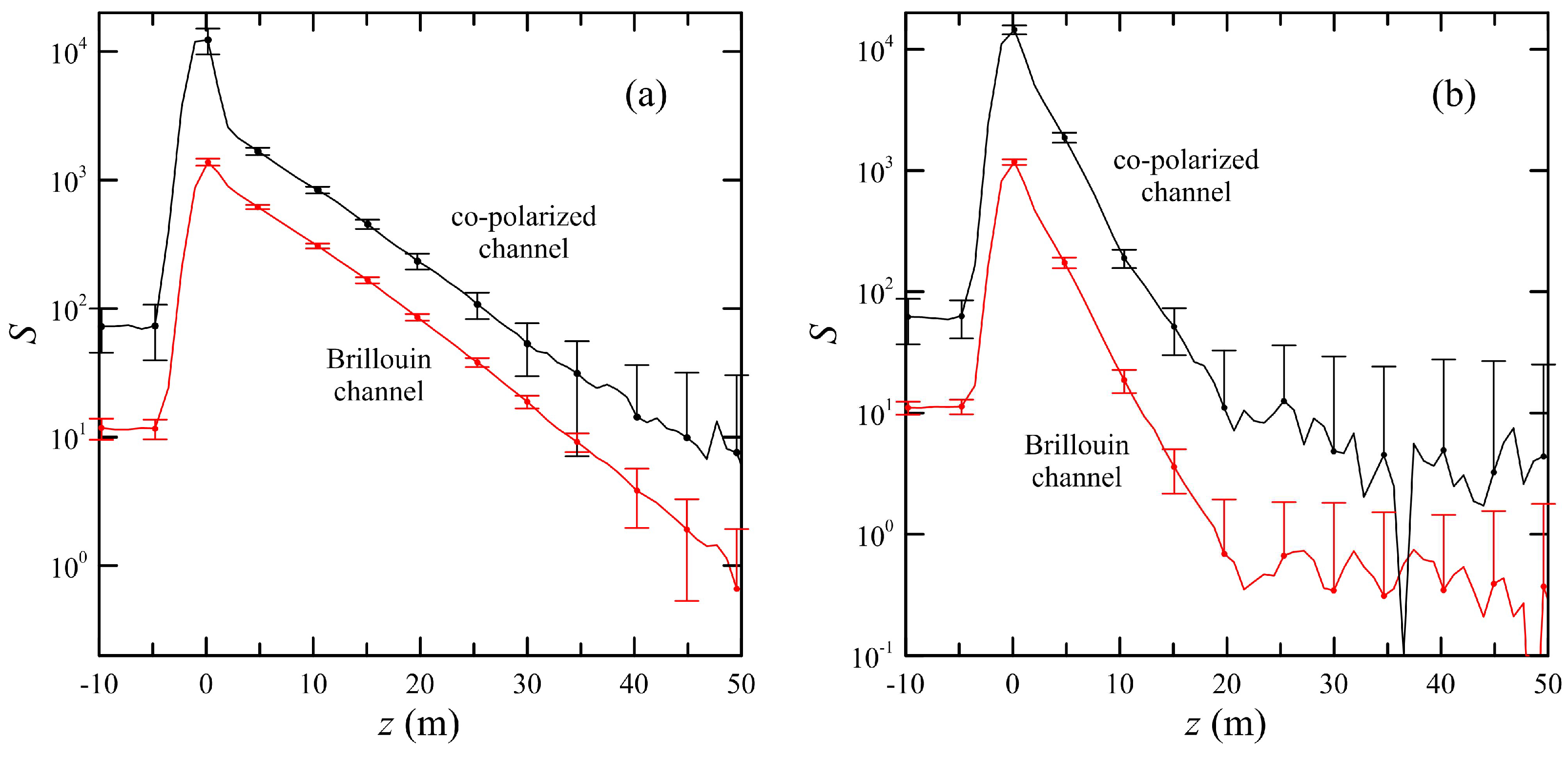
There was generally good agreement between the HPD profiles and PMT profiles, except when the attenuation was high. When the signal drops off rapidly, afterpulsing in the PMTs creates an artificially high signal when the actual signal is low. This effect is not seen in the HPDs, and HPD data will be used in the following analyses. Sample HPD data (Figure 2) show the effects of attenuation coefficient on the return. The left panel presents an open ocean case with an attenuation coefficient of 0.068 m⁻¹ between 5 and 30 m depths. The right panel presents a coastal example with an attenuation coefficient of 0.18 m⁻¹ between 5 and 15 m. The uncertainty in the returns is greater for the co-polarized channel than for the Brillouin channel, despite the lower volume backscattering of the latter, because the collected light is split so that 90% goes into the Brillouin channel and 10% into the co-polarized channel. This has implications for the performance of the PR method, which is only using 10% of the total lidar return.

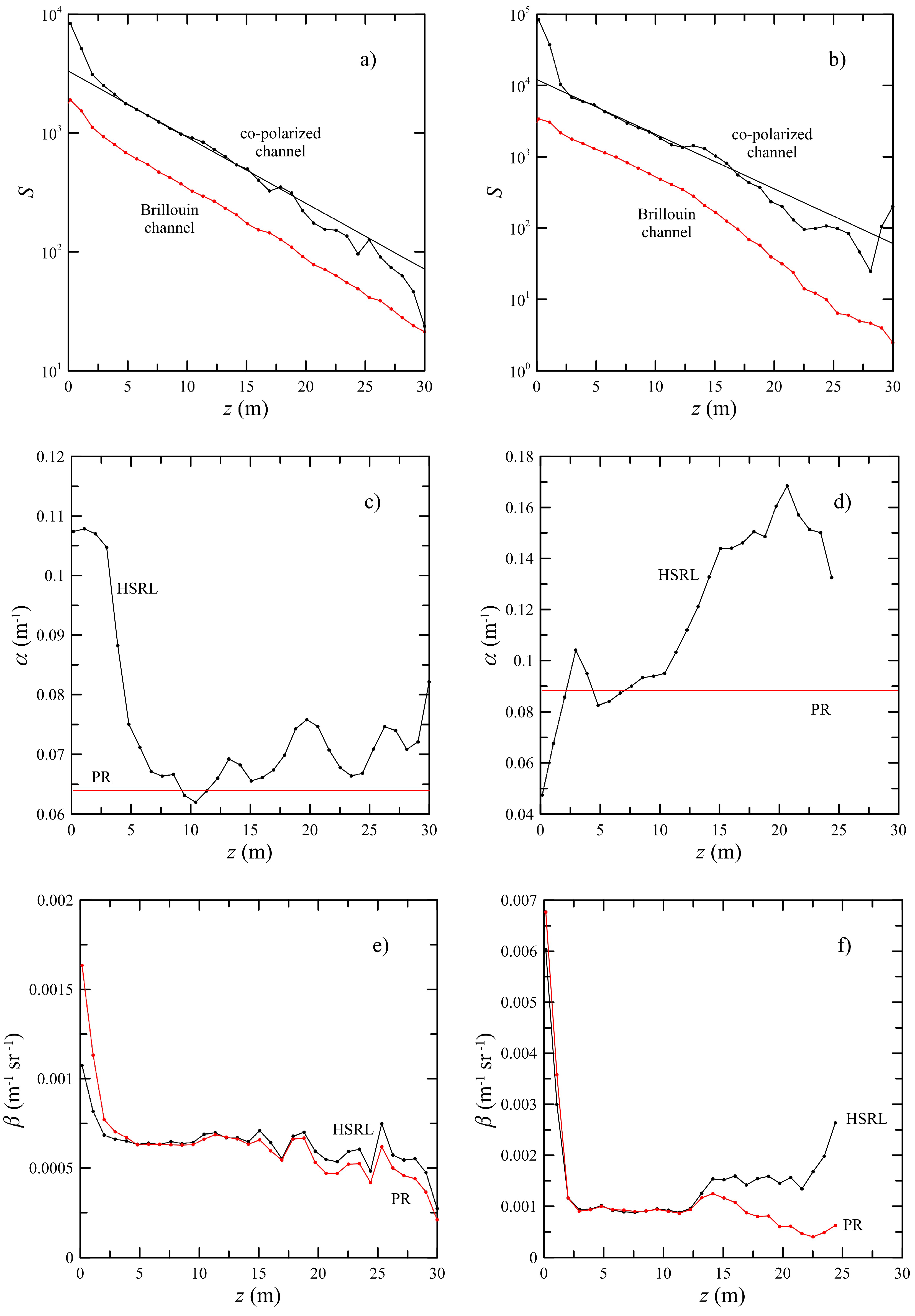
Examples of single profiles and the corresponding retrieved parameters (Figure 3) illustrate the differences between the two methods. On the left is an open-ocean case (65.65°E, 33.58°N), where the optical properties of the water are relatively constant in the upper 30 m, except right at the surface. The surface enhancement in the Brillouin channel is a result of enhanced backscatter induced by surface waves. Curved sections of the surface can partially focus the laser illumination, and scattering from the focus is partially collimated along the reciprocal path. The result is an imperfect cat’s eye retroreflector, leading to an enhanced backscatter. In the co-polarized channel, the enhancement is a combination of enhanced backscatter and specular reflections from surface wave facets at the lidar incidence angle of 15° from nadir. Because of the enhancement in the Brillouin channel, the HSRL attenuation coefficient is probably too large near the surface. At depths from 5 to 30 m, however, the HSRL-derived profile of attenuation is closer to the value obtained from the perturbation retrieval, with an average value that is about 8% higher and a maximum value at 30 m that is 28% higher. Because the surface-wave enhancement affects both HSRL channels, the inferred value for β at the surface is an accurate estimate of the combined specular surface return and near-surface volume backscattering. In this example, a calibration factor was applied to the values for β inferred from the perturbation retrieval to get good agreement at 10 m. With this correction, the perturbation retrieval overestimates β at the surface by 50% in this case. The corrected values for β agree fairly well from 5 to 30 m, with the perturbation retrieval underestimating β by an average of 8%. This increases at greater depths, so the perturbation retrieval underestimates β by an average of 16% between 20 and 30 m.

On the right of Figure 3 is a typical near-shore profile (75.40°E, 36.91°N), where the optical properties of the water are more variable. The water depth at this location is about 28 m, and there is a noticeable change in both attenuation and scattering at a depth of about 13 m. In this example, the enhanced backscatter effect is smaller and the specular reflection is larger. The result is that the HSRL technique does not overestimate the attenuation at the surface, and in fact, may underestimate it somewhat because of the averaging process. Both techniques produce the high surface β values in this case, with a difference of about 12%. Between 2 and 12 m, the techniques produce β values that are within 4% of each other. The perturbation retrieval does not perform as well below the change in water properties, however. The derived values for β are too low by as much as 76%.

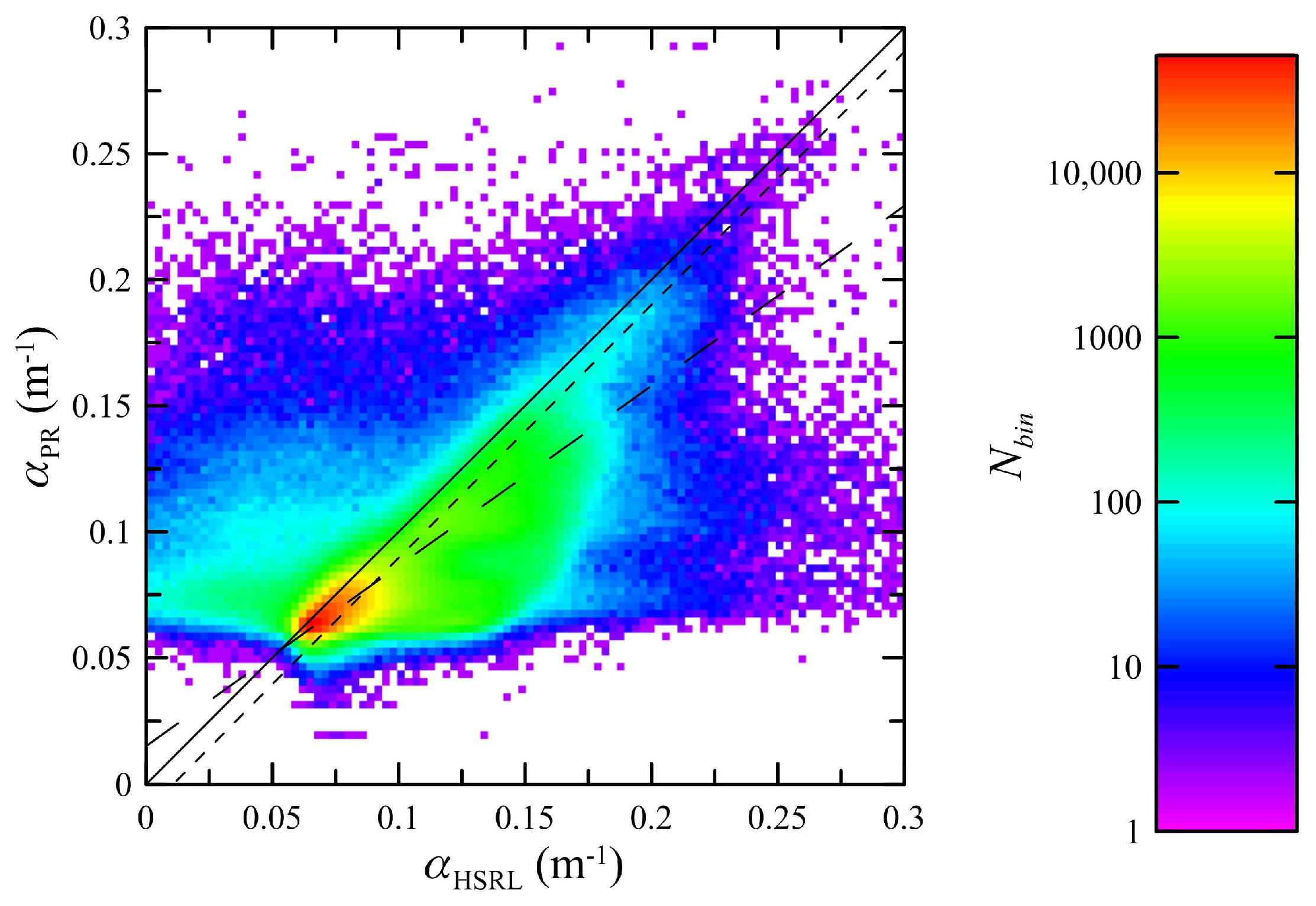
The rest of this section considers statistics of all of the data from the SABOR mission that passed the quality-control measures described above. For example, Figure 4 presents a scatter plot of the lidar attenuation coefficients obtained from the two different processing techniques in offshore waters. The total number of data pairs in this plot was 1,799,238. The Pearson correlation between them was 0.70. While the points are clustered near the one-to-one line, there also numerous points where the PR value is below the HSRL value. Overall, the mean value derived from the PR was 0.079 m⁻¹, and the mean value derived from the HSRL was 0.089 m⁻¹, which represents a relative bias of 11%. The root-mean-square (rms) difference of the two quantities was 0.022 m⁻¹, or about 25% of the HSRL mean. Ordinary least squares regressions were performed using each parameter as the independent variable and the bisector was calculated as recommended in [18]. The bisector regression, given by the long-dashed line in the figure, has a slope of 0.71, which is significantly less than the ideal value of 1. The ordinary regression using the PR values as the independent variable was also plotted as a short dashed line in the figure. There is no good argument for using this regression, but it is interesting that it produces a slope of 1.004 and an intercept of −0.0107 m⁻¹, which is very close to the bias of −0.0100 from the difference of the mean values.

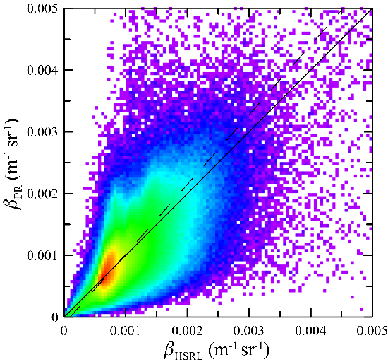
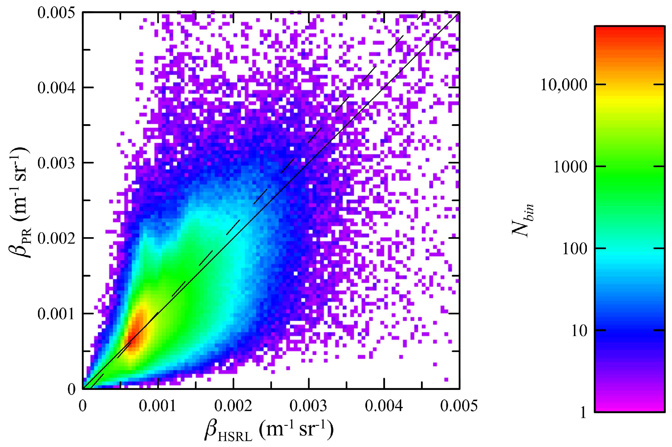
A similar analysis was done for the lidar volume backscattering coefficients (Figure 5). The bisector regression for these data had a slope of 1.13, slightly greater than the ideal slope of 1. The Pearson correlation was about the same as that for the attenuation coefficients, at 0.71. The mean values of volume backscattering were 8.429 × 10⁻⁴ m⁻¹ sr⁻¹ and 8.436 × 10⁻⁴ m⁻¹ sr⁻¹ for the HSRL and PR, respectively. The difference between the mean values was 6.4 × 10⁻⁷ m⁻¹ sr⁻¹, which is <0.1% of the mean values. The bisector regression, shown by the long dashed line, has a slope of 1.13 and an offset of −1.1 × 10⁻⁴ m⁻¹ sr⁻¹. The rms difference between the two quantities was 2.8 × 10⁻⁴ m⁻¹ sr⁻¹, or about 33% of the mean values.

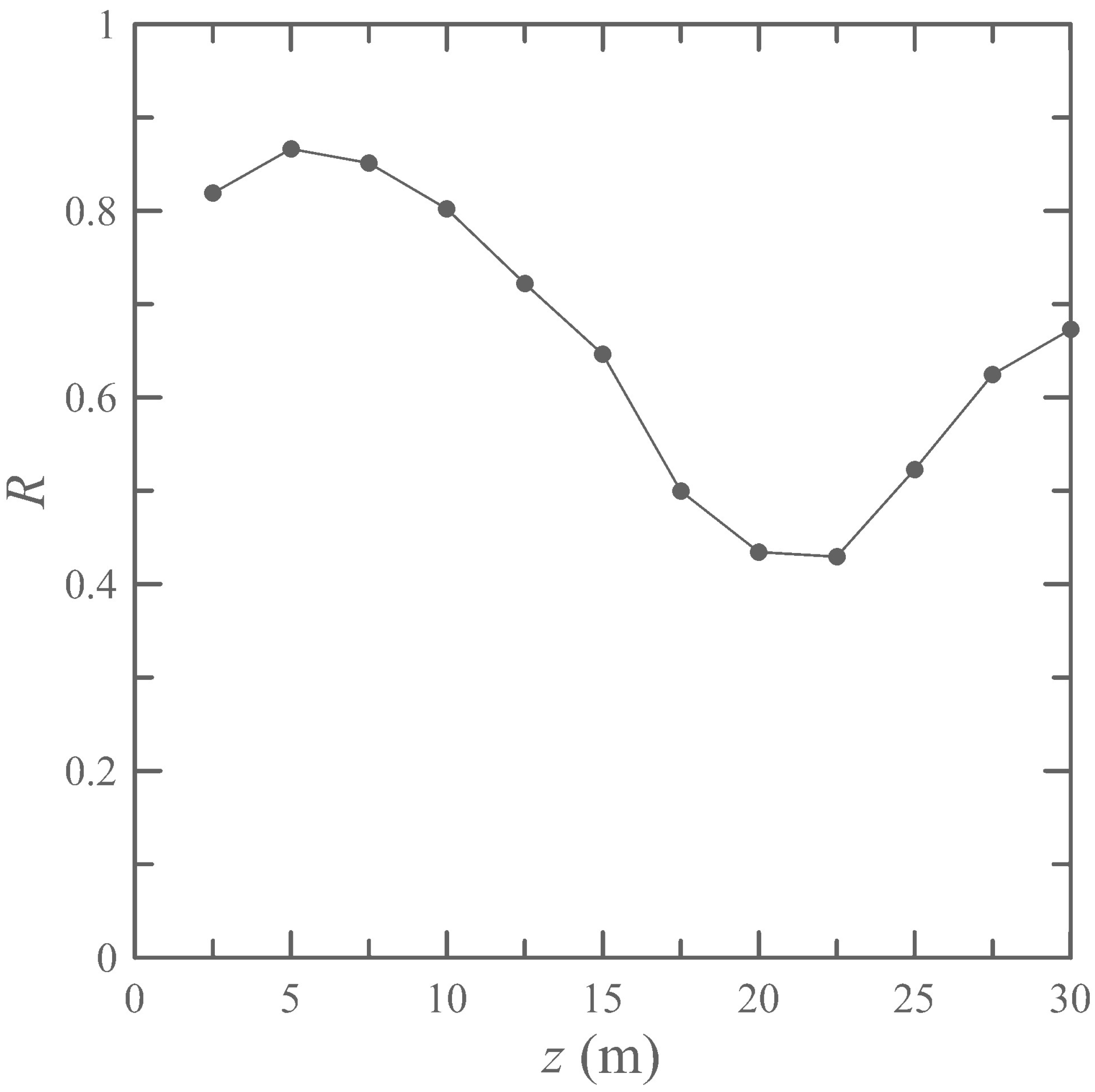
The correlations between the volume backscattering derived from the HSRL processing and derived from the inversion of the co-polarized channel (Figure 6) were calculated at 2.5 m depth intervals down to a depth of 30 m, which was the average penetration depth for the data set. The surface was not included, because of the effects of the Fresnel reflection on the co-polarized channel. Near the surface, where the signal-to-noise ratio is large, the correlation is high. It starts to drop off at about 10 m. Below about 20 m, the correlation begins to increase. This is likely because there are fewer valid near-shore data points at these depths, and the PR performs better in more uniform off-shore waters. Overall, the number of data points used in the correlation at 30 m was only about 66% of that used near the surface.

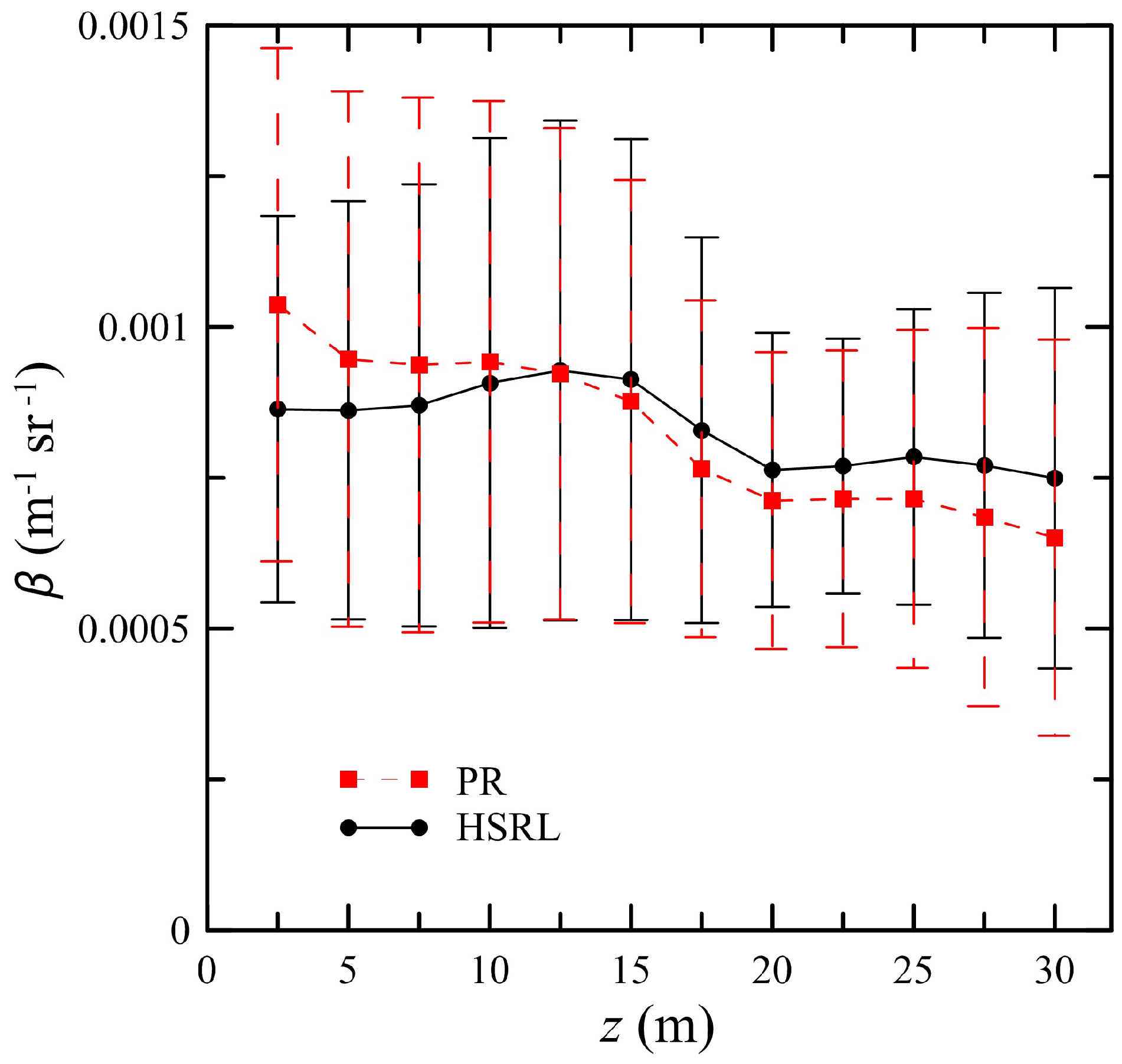
Because of the way the retrieval data were calibrated, the average value for β over all depths was the same for both techniques, although there are differences at different depths (Figure 7). The error bars in the figure represent the standard deviation of data. The relative difference in the means was 13% or less, except for the value at 2.5 m depth. The volume backscattering decreases at depths greater than about 15 m, because regions with very high scattering also had high attenuation, and the penetration depth was less. The low bias in the attenuation coefficient implies that the attenuation correction in the perturbation retrieval of β is generally too low; this produces a bias in the perturbation retrieval of β that is increasingly negative with depth.

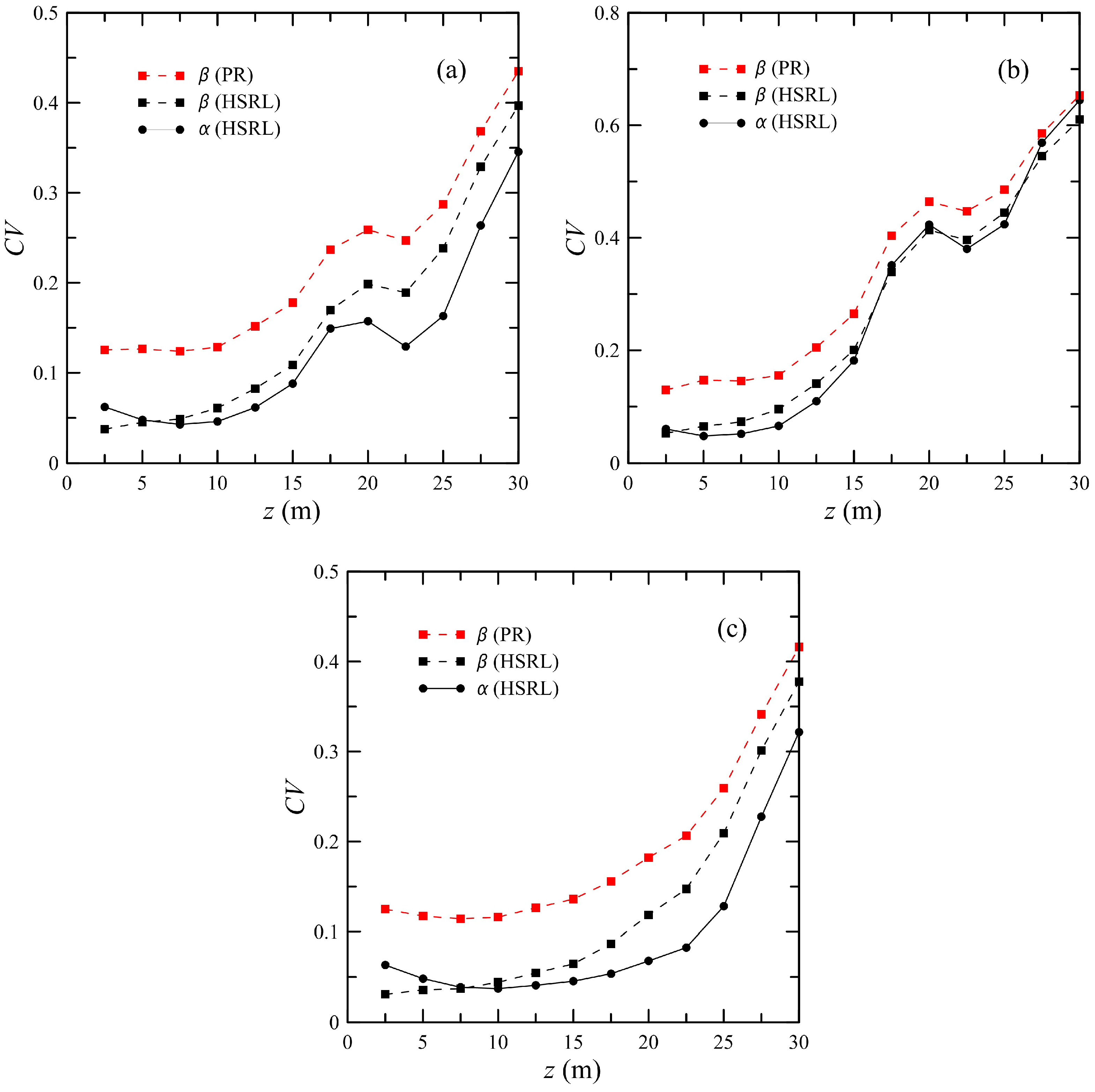
To estimate the relative errors of the two techniques, we calculated the mean and standard deviation data from 100 consecutive profiles at fixed depths. We will consider the coefficient of variation, CV, which is the ratio of the standard deviation to the mean for each quantity at the same 2.5 m depth intervals as before. At each depth, CV was averaged over all of the 100-profile segments. The 100 profiles correspond to about 50 s of data, or 5 km along the flight track. Ideally, the number of profiles used would be enough to get a good estimate of the variability, but the distance would be smaller than the scale of changes in oceanographic conditions. In practice, variability in the ocean occurs over a wide range of scales. In a study using the same data set as this paper, characteristic scales between 200 m and 600 m were inferred [8]. However, previous lidar measurements found a power-law spectrum of the lidar return from constant depths with a slope of −1.5 and no characteristic scale between 5 m and 200 km [19]. While the CV at the shallow depths may include contributions from oceanographic variability, the increase with increasing depth (Figure 8) suggests that the deeper values are dominated by noise effects. The errors in shallower, more turbid waters on the continental shelf are larger than those in deeper waters off shore. Note that there is a local peak in the coastal values at a depth of 20 m. Deeper than this, some of the noisier data are removed from the average, because they are deeper than the local penetration depth.

4. Discussion

A detailed comparison of HSRL and in situ data from SABOR was done previously [7]. That study found that the HSRL estimate of diffuse attenuation coefficient, K_d, was biased high relative to the in situ measurements by about 13%. Here, we found that the HSRL estimate of α, which is equal to K_d for the lidar geometry, was biased high relative to the PR estimate by about 11%. This suggests that the bias relative to in situ measurements might be less for the PR than for the HSRL, although the comparison of in situ data with HSRL used only a portion of the full data set. The rms difference between HSRL and in situ K_d was 17%, which is less than the rms difference between HSRL and PR lidar attenuations of 25% found here. Similarly, the rms difference between particulate backscattering coefficient, b_bp, from HSRL and from in situ measurements (27%) was less than the difference between HSRL and PR volume backscattering (33%).

The results suggest that the PR technique does better in the open ocean than in coastal waters. This is consistent with the results of [14], which found that estimation of scattering profiles through plankton layers using the PR was more accurate when layers were comparatively weak or when the background chlorophyll concentration was low. Both of these conditions are more common in open ocean waters, but can also occur near shore.

One interesting feature of these data is the difference in both α and β near the surface. The explanation is that surface waves produce an enhanced scattering near the surface at a scattering angle of 180° [20,21,22]. The HSRL technique using iodine filters and a laser that has high spectral purity, enables a direct measure of the expected enhanced backscatter near the ocean surface (0–10 m) by removing the ocean surface reflection. The mean enhancement of the Brillouin channel, estimated by comparing the peak return in the channel with the return that would be expected by extrapolating deeper returns back to the surface, was 40%. This is consistent with the results of McLean and Freemen [21], where an enhancement of up to 50% was predicted at a depth of 1 m. Because the enhancement is the same for the Brillouin and co-polarized channels, the HSRL technique is not affected, while the perturbation retrieval overestimates β at 2.5 m as expected. On the other hand, the enhancement affects the HSRL retrieval of attenuation near the surface, while the perturbation retrieval is less affected due to the assumption of a constant attenuation at all depths and because the fit does not use the data near the surface for the regression. This suggests that a more accurate estimate of α at the surface can be obtained from HSRL data by extrapolation from near-surface values not affected by enhanced backscatter. Potentially, this can be improved using an assumed extinction-to-backscatter ratio and the backscatter to get a better estimate.

This analysis does not consider the fact that radiometric calibration of the lidar is required if the HSRL technique is not used. Calibration of atmospheric lidar has been an issue for some time [23,24,25], and is an area of ongoing research. For airborne or space-based oceanographic lidar, the use of known targets like homogeneous land surfaces [26] or the sea surface [27] has been suggested, but these approaches add additional constraints on the lidar system to be used in practice. For the sea surface approach, a satellite measurement of surface winds with an accuracy of 1 m s⁻¹ should be sufficient to provide a calibration to within 10% [27]. Laboratory calibrations rely on the stability of the calibration when the system is deployed along with careful monitoring of the absolute value of the laser energy.

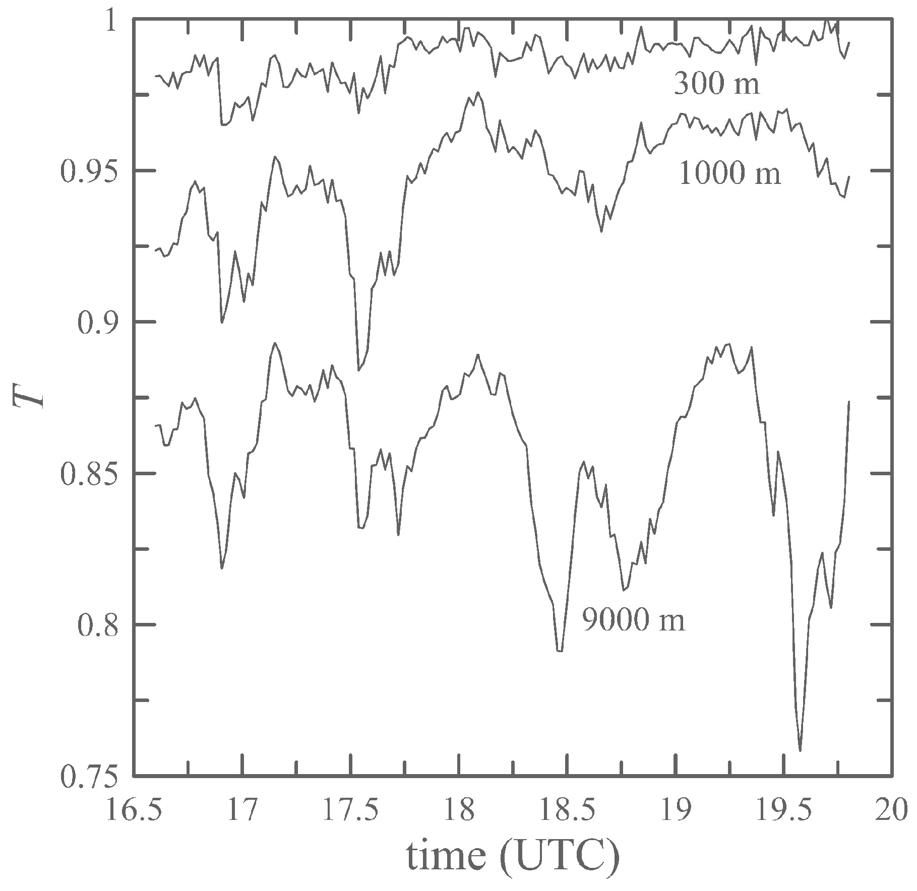
Note that the effects of atmospheric attenuation by aerosols must be considered in the PR retrieval, except at low flight altitudes. For HSRL, this can be accurately estimated using the molecular channel, but is not required to obtain the oceanic parameters. For example, Figure 9 presents the two-way transmission from the aircraft to the surface and back for the first flight. Without the HSRL atmospheric profile, however, estimation of this transmission is generally not possible. For an aircraft at an altitude of 9000 m, the calibration error that would be introduced by neglecting aerosol extinction would be >10% for this entire flight and varying up to 25%. In general, the attenuation will depend on the attenuation down to the surface including aerosol and tenuous clouds (e.g., cirrus clouds). However, for an aircraft flight altitude of 300 m, the calibration error would have been generally <3%, and <10% for an altitude of 1000 m.

5. Conclusions

A perturbation retrieval was compared with HSRL processing to derive a profile of the volume backscattering. For the data set considered, we found that the perturbation retrieval performed better when the water properties were more vertically uniform, as in the oligotrophic waters, than it did near shore where the water tends to be more variable, as expected due to the retrieval assumptions. For the data set investigated, the attenuation coefficient inferred using the perturbation retrieval was biased about 11% low compared with that from the HSRL. The PR estimate of the scattering parameter decreased with depth relative to the HSRL estimate, although the overall bias was zero as a result of the calibration procedure. Near the surface, the coefficient of variability in both estimates of attenuation and in HSRL estimates of scattering were around 5%, but that in the PR estimate of scattering was over 10%. At greater depths, the variability increases for all of the profile parameters. This reflects the effects of increased shot noise at greater depths. The correlation between the two estimates of the attenuation coefficient was 0.7. The correlation between scattering parameters was >0.8 near the surface, but decreased to 0.4 at a depth of around 20 m.

The comparisons were based on data from the same lidar, therefore these results show the improvements in performance that can be expected from the HSRL method in a way that does not depend on the specific characteristics of the lidar. These improvements include reduced bias and reduced sensitivity to noise. Another key advantage is that only relative calibrations between the channels are required, and these can be done within the lidar itself. A standard backscatter lidar requires an estimate of atmospheric attenuation below the aircraft to avoid bias in the ocean retrievals, although these effects can be reduced by operating at lower flight altitudes. The HSRL technique accounts for the effects of atmospheric attenuation directly. The primary disadvantage to the HSRL technique is the requirement for a single-frequency laser and inclusion of an optical filter in the receiver. Both add complexity, and a single-frequency laser will have a lower pulse energy for the same pump energy. Another disadvantage is that the returned light has to be separated into two channels, which decreases the signal to noise ratio relative to a backscatter lidar with the same laser energy. Both techniques are affected by surface roughness, and our results show that the HSRL estimate for attenuation near the surface needs to account for these effects. We showed that the effect can be evaluated using the constant attenuation profile retrieval when conditions are well mixed with depth. This effect may also provide information on the sea surface state given further evaluation.