High-Resolution UAV-Based Hyperspectral Imagery for LAI and Chlorophyll Estimations from Wheat for Yield Prediction


Abstract
1. Introduction
2. Materials and Methods
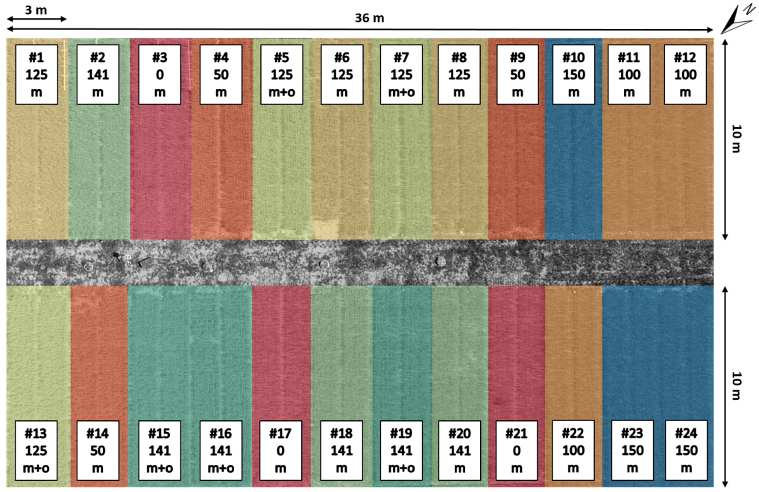
2.1. Study Area and Crop Management
2.2. Data and Preprocessing
2.2.1. Field Data
2.2.2. Hyperspectral UAV Image Data
2.3. Methodology
3. Results
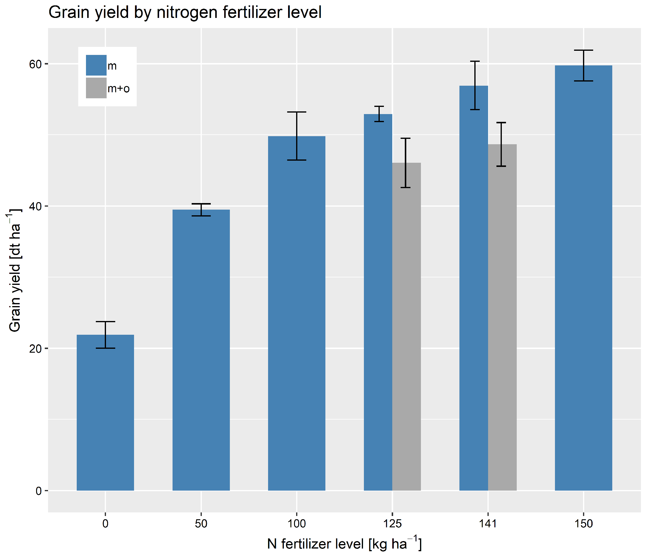
3.1. Data Analysis
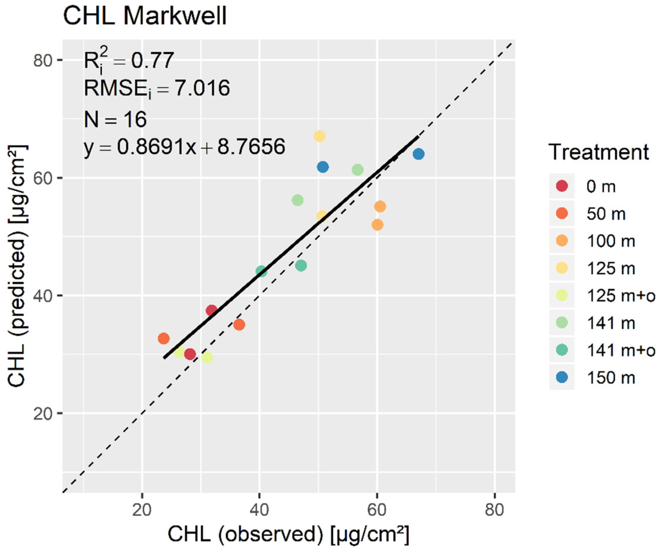
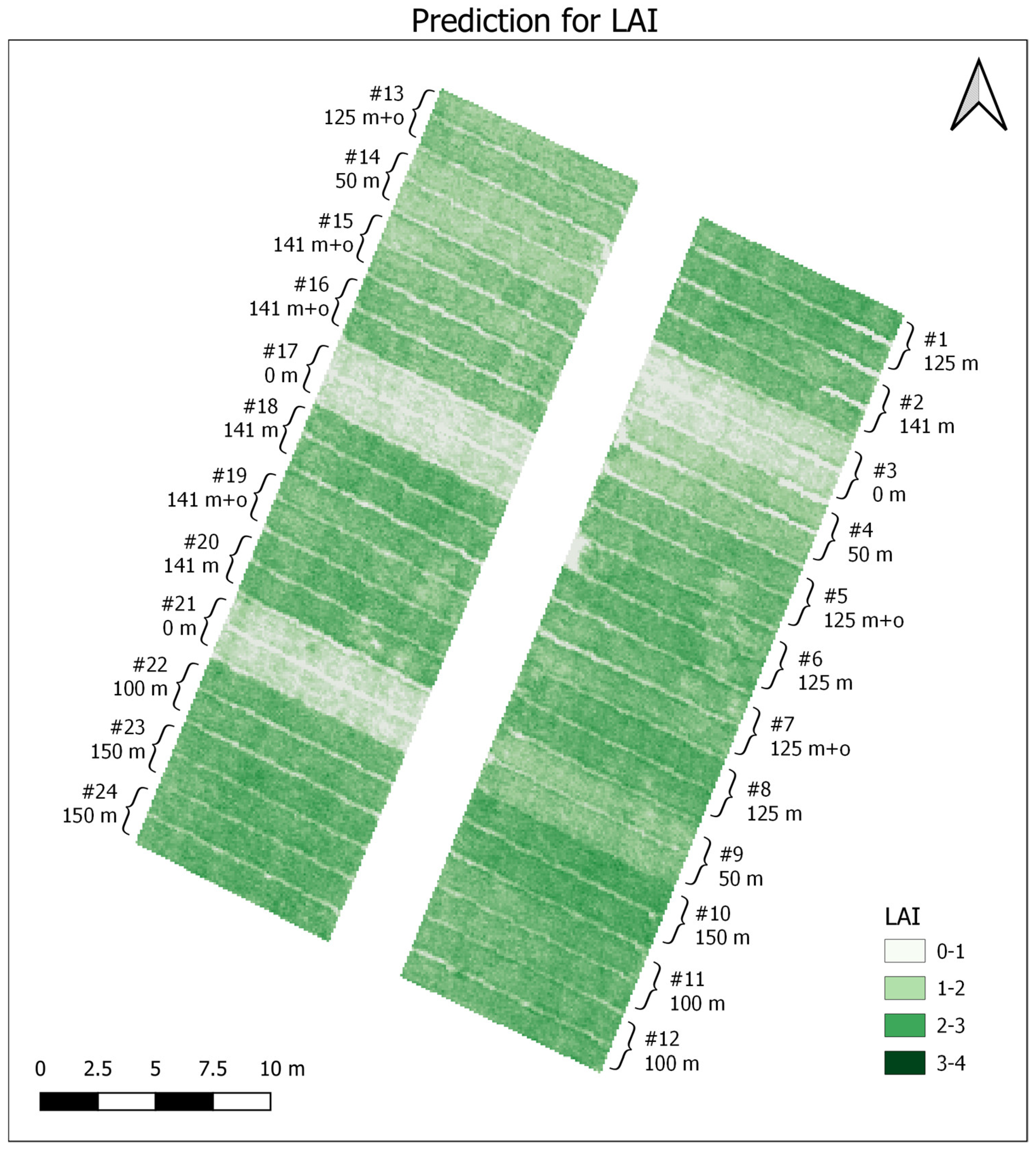
3.2. PLSR and MLR
4. Discussion
5. Conclusions
Author Contributions
Funding
Acknowledgments
Conflicts of Interest
References
- Tilman, D. Global environmental impacts of agricultural expansion: The need for sustainable and efficient practices. Proc. Natl. Acad. Sci. USA 1999, 96, 5995–6000. [Google Scholar] [CrossRef] [PubMed]
- Rütting, T.; Aronsson, H.; Delin, S. Efficient use of nitrogen in agriculture. Nutr. Cycl. Agroecosyst. 2018, 110, 1–5. [Google Scholar] [CrossRef]
- Diacono, M.; Rubino, P.; Montemurro, F. Precision nitrogen management of wheat. A review. Agron. Sustain. Dev. 2013, 33, 219–241. [Google Scholar] [CrossRef]
- Gitelson, A. Remote sensing estimation of crop biophysical characteristics at various scales. In Hyperspectral Remote Sensing of Vegetation; Thenkabail, P.S., Lyon, J.G., Huete, A., Eds.; CRC Press: Boca Raton, FL, USA, 2012; ISBN 978-1-4398-4537-0. [Google Scholar]
- Hunt, E.R.; Daughtry, C.S.T. What good are unmanned aircraft systems for agricultural remote sensing and precision agriculture? Int. J. Remote Sens. 2017, 39, 1–32. [Google Scholar] [CrossRef]
- Aasen, H.; Honkavaara, E.; Lucieer, A.; Zarco-Tejada, P.J. Quantitative remote sensing at ultra-high resolution with UAV spectroscopy: A review of sensor technology, measurement procedures, and data correctionworkflows. Remote Sens. 2018, 10, 1091. [Google Scholar] [CrossRef]
- Manfreda, S.; McCabe, M.F.; Miller, P.E.; Lucas, R.; Madrigal, V.P.; Mallinis, G.; Ben Dor, E.; Helman, D.; Estes, L.; Ciraolo, G.; et al. On the use of unmanned aerial systems for environmental monitoring. Remote Sens. 2018, 10, 641. [Google Scholar] [CrossRef]
- Adão, T.; Hruška, J.; Pádua, L.; Bessa, J.; Peres, E.; Morais, R.; Sousa, J.J. Hyperspectral imaging: A review on UAV-based sensors, data processing and applications for agriculture and forestry. Remote Sens. 2017, 9, 1110. [Google Scholar] [CrossRef]
- Lucieer, A. HyperUAS—Imaging Spectroscopy from a Multirotor Unmanned Aircraft System. J. F. Robot. 2014, 31, 571–590. [Google Scholar] [CrossRef]
- Hruska, R.; Mitchell, J.; Anderson, M.; Glenn, N.F. Radiometric and geometric analysis of hyperspectral imagery acquired from an unmanned aerial vehicle. Remote Sens. 2012, 4, 2736–2752. [Google Scholar] [CrossRef]
- Jaud, M.; Le Dantec, N.; Ammann, J.; Grandjean, P.; Constantin, D.; Akhtman, Y.; Barbieux, K.; Allemand, P.; Delacourt, C.; Merminod, B. Direct georeferencing of a pushbroom, lightweight hyperspectral system for mini-UAV applications. Remote Sens. 2018, 10, 204. [Google Scholar] [CrossRef]
- Calderón, R.; Navas-Cortés, J.A.; Lucena, C.; Zarco-Tejada, P.J. High-resolution airborne hyperspectral and thermal imagery for early detection of Verticillium wilt of olive using fluorescence, temperature and narrow-band spectral indices. Remote Sens. Environ. 2013, 139, 231–245. [Google Scholar] [CrossRef]
- Turner, D.; Lucieer, A.; McCabe, M.; Parkes, S.; Clarke, I. Pushbroom hyperspectral imaging from an Unmanned Aircraft System (UAS)—Geometric processing workflow and accuracy assessment. Int. Arch. Photogramm. Remote Sens. Spat. Inf. Sci.-ISPRS Arch. 2017, 42, 379–384. [Google Scholar] [CrossRef]
- Singh, R. Crop Yield Estimation and Forecasting Using Remote Sensing; Indian Agricultural Statistics Research Institute: New Delhi, India, 2012. [Google Scholar]
- Oøvergaard, S.I.; Isaksson, T.; Kvaalc, K.; Korsaeth, A. Comparisons of two hand-held, multispectral field radiometers and a hyperspectral airborne imager in terms of predicting spring wheat grain yield and quality by means of powered partial least squares regression. J. Near Infrared Spectrosc. 2010, 18, 247–261. [Google Scholar] [CrossRef]
- Herrmann, I.; Vosberg, S.K.; Ravindran, P.; Singh, A.; Chang, H.X.; Chilvers, M.I.; Conley, S.P.; Townsend, P.A. Leaf and canopy level detection of Fusarium virguliforme (sudden death syndrome) in soybean. Remote Sens. 2018, 10, 426. [Google Scholar] [CrossRef]
- Ma, B.L.; Dwyer, L.M.; Costa, C.; Cober, E.R.; Morrison, M.J. Early prediction of soybean yield from canopy reflectance measurements. Agron. J. 2001, 93, 1227–1234. [Google Scholar] [CrossRef]
- Weber, V.S.; Araus, J.L.; Cairns, J.E.; Sanchez, C.; Melchinger, A.E.; Orsini, E. Prediction of grain yield using reflectance spectra of canopy and leaves in maize plants grown under different water regimes. F. Crop. Res. 2012, 128, 82–90. [Google Scholar] [CrossRef]
- Liu, X.; Zhang, K.; Zhang, Z.; Cao, Q.; Lv, Z.; Yuan, Z.; Tian, Y.; Cao, W.; Zhu, Y. Canopy chlorophyll density based index for estimating nitrogen status and predicting grain yield in rice. Front. Plant Sci. 2017, 8, 1–12. [Google Scholar] [CrossRef]
- Muñoz-Huerta, R.F.; Guevara-Gonzalez, R.G.; Contreras-Medina, L.M.; Torres-Pacheco, I.; Prado-Olivarez, J.; Ocampo-Velazquez, R.V. A review of methods for sensing the nitrogen status in plants: Advantages, disadvantages and recent advances. Sensors 2013, 13, 10823–10843. [Google Scholar] [CrossRef]
- Herrmann, I.; Pimstein, A.; Karnieli, A.; Cohen, Y.; Alchanatis, V.; Bonfil, D.J. LAI assessment of wheat and potato crops by VENμS and Sentinel-2 bands. Remote Sens. Environ. 2011, 115, 2141–2151. [Google Scholar] [CrossRef]
- Viña, A.; Gitelson, A.A.; Nguy-Robertson, A.L.; Peng, Y. Comparison of different vegetation indices for the remote assessment of green leaf area index of crops. Remote Sens. Environ. 2011, 115, 3468–3478. [Google Scholar] [CrossRef]
- Siegmann, B.; Jarmer, T. Comparison of different regression models and validation techniques for the assessment of wheat leaf area index from hyperspectral data. Int. J. Remote Sens. 2015, 36, 4519–4534. [Google Scholar] [CrossRef]
- Darvishzadeh, R.; Skidmore, A.; Schlerf, M.; Atzberger, C.; Corsi, F.; Cho, M. LAI and chlorophyll estimation for a heterogeneous grassland using hyperspectral measurements. ISPRS J. Photogramm. Remote Sens. 2008, 63, 409–426. [Google Scholar] [CrossRef]
- Goel, P.K.; Prasher, S.O.; Patel, R.M.; Viau, A.A.; Miller, J.R. Estimation of crop biophysical parameters through airborne and field hyperspectral remote sensing. Trans. ASAE 2003, 46, 1235–1246. [Google Scholar]
- Atzberger, C.; Darvishzadeh, R.; Immitzer, M.; Schlerf, M.; Skidmore, A.; le Maire, G. Comparative analysis of different retrieval methods for mapping grassland leaf area index using airborne imaging spectroscopy. Int. J. Appl. Earth Obs. Geoinf. 2015, 43, 19–31. [Google Scholar] [CrossRef]
- Jarmer, T. Spectroscopy and hyperspectral imagery for monitoring summer barley. Int. J. Remote Sens. 2013, 34, 6067–6078. [Google Scholar] [CrossRef]
- Yue, J.; Feng, H.; Jin, X.; Yuan, H.; Li, Z.; Zhou, C.; Yang, G.; Tian, Q. A comparison of crop parameters estimation using images from UAV-mounted snapshot hyperspectral sensor and high-definition digital camera. Remote Sens. 2018, 10, 1138. [Google Scholar] [CrossRef]
- Yuan, H.; Yang, G.; Li, C.; Wang, Y.; Liu, J.; Yu, H.; Feng, H.; Xu, B.; Zhao, X.; Yang, X. Retrieving soybean leaf area index from unmanned aerial vehicle hyperspectral remote sensing: Analysis of RF, ANN, and SVM regression models. Remote Sens. 2017, 9, 309. [Google Scholar] [CrossRef]
- Zarco-Tejada, P.J.; Miller, J.R.; Morales, A.; Berjón, A.; Agüera, J. Hyperspectral indices and model simulation for chlorophyll estimation in open-canopy tree crops. Remote Sens. Environ. 2004, 90, 463–476. [Google Scholar] [CrossRef]
- Atzberger, C.; Guérif, M.; Baret, F.; Werner, W. Comparative analysis of three chemometric techniques for the spectroradiometric assessment of canopy chlorophyll content in winter wheat. Comput. Electron. Agric. 2010, 73, 165–173. [Google Scholar] [CrossRef]
- Blackburn, G.A. Quantifying chlorophylls and caroteniods at leaf and canopy scales. Remote Sens. Environ. 1998, 66, 273–285. [Google Scholar] [CrossRef]
- Mozgeris, G.; Jonikavičius, D.; Jovarauskas, D.; Zinkevičius, R.; Petkevičius, S.; Steponavičius, D. Imaging from manned ultra-light and unmanned aerial vehicles for estimating properties of spring wheat. Precis. Agric. 2018, 19, 876–894. [Google Scholar] [CrossRef]
- Peel, M.C.; Finlayson, B.L.; McMahon, T.A. Updated world map of the Köppen-Geiger climate classification. Hydrol. Earth Syst. Sci. 2007, 11, 1633–1644. [Google Scholar] [CrossRef]
- Deutscher Wetterdienst (DWD) Climate Dataset—Archive Data Station 342 Belm. Available online: http://www.dwd.de (accessed on 5 October 2017).
- LWK-NDS: Chamber of Agriculture Lower Saxony Plant Production and Plant Protection—Recommendations; Landwirtschaftskammer Niedersachsen: Hannover, Gernany, 2016.
- Markwell, J.; Osterman, J.C.; Mitchell, J.L. Calibration of the Minolta SPAD-502 leaf chlorophyll meter. Photosynth. Res. 1995, 46, 467–472. [Google Scholar] [CrossRef] [PubMed]
- Smith, G.M.; Milton, E.J. The use of the empirical line method to calibrate remotely sensed data to reflectance. Int. J. Remote Sens. 1999, 20, 2653–2662. [Google Scholar] [CrossRef]
- Green, A.A.; Berman, M.; Switzer, P.; Craig, M.D. A Transformation for Ordering Multispectral Data in Terms of Image Quality with Implications for Noise Removal. IEEE Trans. Geosci. Remote Sens. 1988, 26, 65–74. [Google Scholar] [CrossRef]
- Geladi, P.; Kowalski, B.R. Partial least-squares regression: Q tutorial. Anal. Chim. Acta 1986, 185, 1–17. [Google Scholar] [CrossRef]
- Hocking, A.R.R. The Analysis and Selection of Variables in Linear Regression. Biometrics 1976, 32, 1–49. [Google Scholar] [CrossRef]
- Otto, M. Chemometrics: Statistics and Computer Application in Analytical chemistry, 3rd ed.; John Wiley & Sons: Weinheim, Germany, 2016. [Google Scholar]
- R Core Team R: A Language and Environment for Statistical Computing. Available online: https://www.r-project.org (accessed on 10 December 2018).
- Zadoks, J.; Chang, T.; Konzak, C. A decimal growth code for the growth stages of cereals. Weed Res. 1974, 14, 415–421. [Google Scholar] [CrossRef]
- Lazauskas, S.; Povilaitis, V.; Antanaitis, S.; Sakalauskaitė, J.; Sakalauskienė, S.; Pšibišauskienė, G.; Auškalnienė, O.; Raudonius, S.; Duchovskis, P. Winter wheat leaf area index under low and moderate input management and climate change. J. Food Agric. Environ. 2012, 10, 588–593. [Google Scholar]
- Skudra, I.; Ruza, A. Effect of nitrogen and sulphur fertilization on chlorophyll content in winter wheat. Rural Sustain. Res. 2017, 37. [Google Scholar] [CrossRef]
- Serrano, L.; Filella, I.; Peñuelas, J. Remote sensing of biomass and yield of winter wheat under different nitrogen supplies. Crop Sci. 2000, 40, 723. [Google Scholar] [CrossRef]
- Horler, D.N.H.; Dockray, M.; Barber, J. The red edge of plant leaf reflectance. Int. J. Remote Sens. 1983, 4, 273–288. [Google Scholar] [CrossRef]
- Schlerf, M.; Atzberger, C.; Hill, J. Remote sensing of forest biophysical variables using HyMap imaging spectrometer data. Remote Sens. Environ. 2005, 95, 177–194. [Google Scholar] [CrossRef]
- Curran, P.J. Remote Sensing of Foliar Chemistry. Remote Sens. Environ. 1989, 30, 271–278. [Google Scholar] [CrossRef]
- Haynes, R. Mineral Nitrogen in the Plant-Soil System; Academic Press: New York, NY, USA, 2012. [Google Scholar]


| Winter Wheat | |
|---|---|
| Sowing date | 14.10.2016 |
| Variety | Anapolis |
| Seeding rate | 300 grains m−2 |
| Harvest date | 31.07.2017 (290 DAS) |
| Soil type | Stagnic Anthrosol |
| Soil mineral nitrogen before sowing | 49 kg ha−1 |
| N-Application | First 152 DAS (tillering) Second 187 DAS (stem elongation) Third 220 DAS (booting) |
| N level | 0 | 50 | 100 | 125 (opt–) | 141 (opt) | 150 | ||
|---|---|---|---|---|---|---|---|---|
| N type | m | m | m | m | m + o | m | m + o | m |
| First application | - | 29 | 29 | 50 | 47 + 20 | 54 | 47 + 20 | 43 |
| Second application | - | 21 | 43 | 25 | 38 + 20 | 33 | 47 + 27 | 64 |
| Third application | - | - | 28 | 50 | - | 54 | - | 43 |
| Soil mineral nitrogen | 49 | 49 | 49 | 49 | 49 | 49 | 49 | 49 |
| Sum | 49 | 99 | 149 | 174 | 174 | 190 | 190 | 199 |
© 2018 by the authors. Licensee MDPI, Basel, Switzerland. This article is an open access article distributed under the terms and conditions of the Creative Commons Attribution (CC BY) license (http://creativecommons.org/licenses/by/4.0/).
Share and Cite
Kanning, M.; Kühling, I.; Trautz, D.; Jarmer, T. High-Resolution UAV-Based Hyperspectral Imagery for LAI and Chlorophyll Estimations from Wheat for Yield Prediction. Remote Sens. 2018, 10, 2000. https://doi.org/10.3390/rs10122000
Kanning M, Kühling I, Trautz D, Jarmer T. High-Resolution UAV-Based Hyperspectral Imagery for LAI and Chlorophyll Estimations from Wheat for Yield Prediction. Remote Sensing. 2018; 10(12):2000. https://doi.org/10.3390/rs10122000
Chicago/Turabian StyleKanning, Martin, Insa Kühling, Dieter Trautz, and Thomas Jarmer. 2018. "High-Resolution UAV-Based Hyperspectral Imagery for LAI and Chlorophyll Estimations from Wheat for Yield Prediction" Remote Sensing 10, no. 12: 2000. https://doi.org/10.3390/rs10122000
APA StyleKanning, M., Kühling, I., Trautz, D., & Jarmer, T. (2018). High-Resolution UAV-Based Hyperspectral Imagery for LAI and Chlorophyll Estimations from Wheat for Yield Prediction. Remote Sensing, 10(12), 2000. https://doi.org/10.3390/rs10122000