Article

Evaluation of the Weak Constraint Data Assimilation Approach for Estimating Turbulent Heat Fluxes at Six Sites

1
State Key Laboratory of Earth Surface Processes and Resource Ecology, School of Natural Resources, Faculty of Geographical Science, Beijing Normal University, Beijing 100875, China
2
Department of Civil and Environmental Engineering and Water Resources Research Center, University of Hawaii at Manoa, Honolulu, HI 96822, USA
3
Daugherty Water for Food Global Institute, University of Nebraska, Lincoln, NE 68588, USA
4
Joint Center for Satellite Data Assimilation (JCSDA), College Park, MD 20740, USA
5
University Corporation for Atmospheric Research (UCAR), Boulder, CO 80301, USA
6
College of Water Sciences, Beijing Key Laboratory of Urban Hydrological Cycle and Sponge City Technology, Beijing Normal University, Beijing 100875, China
7
National Hulunber Grassland Ecosystem Observation and Research Station, Institute of Agricultural Resources and Regional Planning, Chinese Academy of Agricultural Sciences, Beijing 100081, China
8
State Key Laboratory of Remote Sensing Science, Faculty of Geographical Science, Beijing Normal University, Beijing 100875, China
*
Author to whom correspondence should be addressed.
Remote Sens. 2018, 10(12), 1994; https://doi.org/10.3390/rs10121994
Submission received: 10 October 2018 / Revised: 12 November 2018 / Accepted: 5 December 2018 / Published: 9 December 2018
(This article belongs to the Section Biogeosciences Remote Sensing)

Abstract

:
A number of studies have estimated turbulent heat fluxes by assimilating sequences of land surface temperature (LST) observations into the strong constraint-variational data assimilation (SC-VDA) approaches. The SC-VDA approaches do not account for the structural model errors and uncertainties in the micrometeorological variables. In contrast to the SC-VDA approaches, the WC-VDA approach (the so-called weak constraint-VDA) accounts for the effects of structural and model errors by adding a model error term. In this study, the WC-VDA approach is tested at six study sites with different climatic and vegetative conditions. Its performance is also compared with that of SC-VDA at the six study sites. The results show that the WC-VDA produces 10.16% and 10.15% lower root mean square errors (RMSEs) for sensible and latent heat flux estimates compared with the SC-VDA approach. The model error term can capture errors in the turbulent heat flux estimates due to errors in LST and micrometeorological measurements, as well as structural model errors, and does not allow those errors to adversely affect the turbulent heat flux estimates. The findings also indicate that the estimated model error term varies reasonably well, so as to capture the misfit between predicted and observed net radiation in different hydrological and vegetative conditions. Finally, synthetically generated positive (negative) noises are added to the hydrological input variables (e.g., LST, air temperature, air humidity, incoming solar radiation, and wind speed) to examine whether the WC-VDA approach can capture those errors. It was found that the WC-VDA approach accounts for the errors in the input data and reduces their effect on the turbulent heat flux estimates.

1. Introduction

Accurate estimation of turbulent heat fluxes (sensible and latent heat fluxes) is required in agricultural, hydrological, and meteorological applications [1,2,3]. Flux towers have been installed across the world to measure turbulent heat fluxes. However, they are expensive and have a sparse distribution (i.e., limited spatial representation). Consequently, a number of models have been developed to estimate turbulent heat fluxes based on in-situ and remotely sensed observations [4,5,6,7,8,9,10,11,12,13].
Land surface temperature (LST) lies at the heart of the surface energy balance (SEB) equation, and has been used in many studies to estimate turbulent heat fluxes [14]. The existing methods for estimating turbulent heat fluxes based on LST observations are mainly divided into five groups. The first group (known as the triangle method) uses the empirical relationship between LST and vegetation indices to predict sensible (H) and latent (LE) heat fluxes [7,15,16,17,18,19,20]. The second group (called the diagnostic approach) obtains sensible and latent heat fluxes by solving the SEB equation [5,6,8,11,13,21,22]. The third group (known as the surface temperature initiated closure method) estimates turbulent heat fluxes by integrating LST observations into the Penman-Monteith equation [23,24]. The fourth group combines hydrological variables (e.g., soil moisture and temperature, vegetation properties, topography, and meteorological forcing data) with a land surface model (e.g., Noah) within an Ensemble Kalman Filter (EnKF) method to predict sensible and latent heat fluxes [25,26,27,28,29,30,31].
The fifth group assimilates sequences of LST observations into the four dimensional variational data assimilation (4D-VDA) frameworks to retrieve H and LE [32,33,34,35,36,37,38,39,40]. This group estimates sensible and latent heat fluxes even for instances in which there are no LST data. The VDA approaches can obtain the key parameters of the land surface control on the partitioning of the available energy between H and LE [i.e., neutral bulk heat transfer coefficient (CHN) and evaporative fraction (EF)]. CHN scales the sum of the turbulent heat fluxes (i.e., H + LE), is mainly a function of vegetation phenology, and is assumed to vary on a monthly time scale. EF scales partitioning between the turbulent heat fluxes (i.e., EF = LE/(H + LE)), and is assumed to be invariant during the assimilation window (i.e., 0900–1800 LT) in each day.
The studies in the fifth group often have used the strong constraint-VDA (SC-VDA) approach that presumes the model structure is perfect and the input data have no errors. However, the simplistic assumptions (e.g., constant daily EF and constant monthly CHN) cause structural model errors in the VDA approaches. Moreover, there are errors in the micrometeorological input variables, and uncertainties in the specifications of the input parameters (e.g., albedo, soil emissivity, and soil thermal properties). Bateni et al. [35] and Xu et al. [38] added a model error term (ω) to the SEB equation within the VDA system [the so-called weak constraint-VDA (WC-VDA) methodology] to account for the errors resulting from uncertainties in the micrometeorological input variables, inaccurate model parameters, and simplistic model parameterizations. They tested the WC-VDA approach at the First International Satellite Land Surface Climatology Project Field Experiment (FIFE) and Huazhaizi sites. Both of these sites are subhumid grasslands.
The objectives of this study were to (1) evaluate the performance of the WC-VDA approach at six sites with different climatic and vegetative conditions, (2) compare the results of WC-VDA to those of SC-VDA, and (3) assess behavior of the model error term under different hydrological and vegetative conditions. This paper is organized as follows: Section 2 introduces the methodology including the heat diffusion equation, SEB equation, and adjoint state formulation; Section 3 explains the study area and data; results and discussions are given in Section 4; and finally, conclusions are reported in Section 5.

2. Methodology

2.1. Heat Diffusion Equation

The heat diffusion equation describes the variation in soil temperature (T) with depth z and time t, and is given by,
C T ( z , t ) t = K 2 T ( z , t ) z 2 ,
where C and K are the soil volumetric heat capacity (J·m−3·K−1) and thermal conductivity (W·m−1·K−1), respectively. To solve the heat diffusion equation, the boundary conditions at the top and bottom of the soil column need to be specified. The boundary condition at the top of the soil column is obtained by the land surface forcing,
K d T ( z = 0 , t ) d z = G ( t ) ,
where G(t) is the ground heat flux at the land surface at time t. At the bottom boundary of the soil column, a Neumann boundary condition, is implemented as
T ( l , t ) z = 0 ,
where l is the depth of the bottom boundary. According to Hu and Islam [41], the soil temperature at the depth of 0.3–0.5 m is almost invariant in a daily time-scale. Hence, l = 0.5 m was used in this study. The soil temperature profile is estimated by integrating the heat diffusion equation from a starting time (τ0),
f ( z , τ 0 ) = f 1 ( z ) ,
where f1(z) represents the soil temperature profile at the initial time (τ0). The readers are referred to Bateni et al. [35] for a detailed description of obtaining f1(z).

2.2. Surface Energy Balance (SEB) equation

The model error term (ω) was added to the SEB equation as follows,
R n = H + LE +   G + ω ( t ) ,
where H and LE are the sensible and latent heat fluxes, respectively. ω(t) is the model error term, which accounts for the model and observation errors, and Rn is the net radiation (W·m−2) that can be defined as,
R n = ( 1 α ) R S + R L ε σ T 4 ,
where α is the surface albedo (–), R S and R L are the incoming shortwave and longwave radiations (W·m−2), respectively, ε is the surface emissivity (–), σ is the Stefan-Boltzmann constant (5.67 × 10⁻⁸ W· m−2·K−4).
The sensible heat flux can be calculated via
H = ρ c P C H U ( T T a ) ,
where ρ is the air density (kg·m−3), CP is the air heat capacity (1012 J·kg−1·K−1), and U and Ta are the reference-height wind speed (m·s−1) and air temperature (K), respectively. Bulk heat transfer coefficient (CH) is related to the heat transfer coefficient under neutral atmospheric condition (CHN) and the atmospheric stability correction function (f(Ri)) via [36,38,40,42],
C H = C H N f ( R i ) = C H N [ 1 + 2 ( 1 e 10 R i ) ] ,
where Ri is the Richardson number. CHN depends on the geometry of the land surface and constitutes the first unknown parameter of the WC-VDA scheme. CHN is assumed to vary on a monthly (30-day) time scale.
Evaporative fraction (EF) is the second unknown parameter of the WC-VDA approach. It is almost constant for near-peak radiation hours on days without precipitation [43]. In this study, EF was assumed to be constant during the assimilation window (0900–1800 LT),
EF = LE / ( H + LE ) ,

2.3. Adjoint State Formulation

The key unknown parameters (CHN and EF) and the model error term (ω) in the WC-VDA approach were obtained by minimizing the cost function J, which is defined as follows,
J ( T , R , EF , λ ) = i = 1 N t 0 t 1 [ T O B S , i ( t ) T i ( t ) ] T R T 1 [ T O B S , i ( t ) T i ( t ) ] d t + ( R R ) T B R 1 ( R R ) + i = 1 N ( EF i EF i ) T B EF 1 ( EF i EF i ) + 2 i = 1 N t 0 t 1 0 l λ i ( z , t ) [ T i ( z , t ) t ( K C ) T i ( z , t ) 2 z 2 ] d z d t + i = 1 N t 0 t 1 t 0 t 1 ω i ( t ) Q ω 1 ( t , t ) ω i ( t ) d t d t ,
where N is the total number of LST observations during the assimilation period, and R T 1 is the inverse covariance matrix of LST observation errors, B R 1 and B EF 1 are the inverse background error covariance matrices of R and EF, respectively, and Q ω 1 is the inverse model error covariance matrix. The first term on the right-hand side of the cost function represents the misfit between the LST observations and predictions. The second and third terms represent the misfit between the parameters estimates (R and EF) and their prior values ( R and EF i ). CHN is related to R via CHN = exp(R) to make it strictly positive and meaningful. The key unknown parameters (CHN and EF) and the model error term (ω) were obtained by minimizing the difference between the LST observations and predictions from the heat diffusion equation. Following Bateni et al. [35], R T 1 , B R 1 , and B EF 1 are assumed to be diagonal matrices of numerically constant values whose relative magnitude controls the rate of convergence of the iterative minimization procedure explained in Appendix A. The magnitudes of the diagonal elements in R T 1 , B R 1 , and B EF 1 are set to 0.01 K−2, 1000, and 1000, respectively [34,35]. The fourth term is the heat diffusion equation (the physical constraint), which is adjoined to the cost function via the Lagrange multiplier Λ. The last term adds the model error (ω(t)) to the objective function to account for the uncertainties in the forcing as well as the parametric and structural model errors. Following Bateni et al. [35], Xu et al. [37], and Reichle [44], the inverse model error covariance can be expressed as,
Q ω 1 ( t , t ) = σ ω 2 exp ( | t t | / τ ) .
This type of error covariance model is often used when the covariance structure of errors is poorly known [44,45]. More information about the weak constraint VDA approach and the model error term based on the Bayes’ theorem can be found in Rodgers [46] and Tremolet [47]. The σω and τ are the standard deviation and decorrelation timescale, which are set to 100 W·m−2 and 6 h, respectively [35]. The strong constraint-VDA (SC-VDA) approach does not include the model error term and treats the physical model as perfect. While, the weak constraint-VDA incorporates the model error term (ω) into the cost function J to account for model uncertainties.
The optimal values of CHN, EF, and ω were obtained by setting the first variation of J to zero (i.e., δJ = 0). Imposing δJ = 0 leads to a number of Euler-Lagrangian equations (shown in Appendix B), which should be solved simultaneously through an iterative procedure to obtain optimal values for CHN, EF, and ω.
The Bias and Root Mean Square Error (RMSE) metrics were used to access the performances of the VDA approach,
B I A S = i = 1 N ( P i O i ) N ,
R M S E = 1 N i = 1 N ( P i O i ) 2 ,
where P i and O i are the predicted and observed values at time step i, respectively.

3. Study Domain and Data

The WC-VDA approach was tested at the Mead, Audubon, Brookings, and Willow Creek sites (Day of Year (DOY) 121–273, 2005) in the US (http://ameriflux.lbl.gov/) [48], as well as the Arou and Desert sites (DOY 121–273, 2015) in China [3,49,50] (http://card.westgis.ac.cn/). Characteristics of these sites are summarized in Table 1. The experimental sites have four vegetation cover types: grassland, cropland, forest, and barren land. Mead is an irrigated cropland. Willow Creek is a deciduous broadleaf forest with dense vegetation cover (high leaf area index, LAI). Arou, Audubon, and Brookings are grasslands with a large range of soil moisture (0.07–0.45 m3·m−3) and LAI (0.39–2.53 m2·m−2). Desert is barren land with sparse vegetation and dry soil. The wide range of soil moisture and LAI values allows us to assess performance of the WC-VDA approach and variations of the model error term under different environmental conditions.
The half-hourly micrometeorological data (wind speed, air temperature and humidity, incoming shortwave and longwave radiations) were measured at the six sites by Automatic Weather Stations (AWS). At all the sites, the sensible and latent heat fluxes were measured by the eddy covariance (EC) instrument. Albedo and LAI data were obtained from the Global Land Surface Satellite (GLASS) product [51,52] (http://glass-product.bnu.edu.cn/). The soil heat capacity (C) and conductivity (K) depend on the soil moisture and texture [53,54,55]. In this study, soil texture and moisture at each site were obtained from the Harmonized World Soil Database (HWSD) and Heihe River Basin (HRB) Digital Soil Mapping product, respectively [56].

4. Results and Discussions

4.1. Neutral Bulk Heat Transfer Coefficient

Table 2 represents the neutral bulk heat transfer coefficient (CHN) estimates and LAI values for the six experimental sites. As shown, changes in the CHN estimates are consistent with those of LAI. The CHN values are generally higher at the densely vegetated sites (Arou, Brookings, and Willow Creek), and lower at the sparsely vegetated sites (Audubon and Desert). At the Mead site, CHN increases with the growth of the crop and reaches its maximum in the fourth period (DOY 213–243) where LAI is at its peak value. The higher CHN value at the Willow Creek site is attributed to its dense vegetation cover (LAI = 4.8). There is no vegetation coverage at the Desert site (LAI is zero), and hence the CHN estimates at Desert are lower than those of the other sites. Although LAI is invariant at the Desert site, the CHN estimates vary in different monthly modeling periods. This is because CHN depends on not only vegetation phenology (LAI) but also wind speed, friction velocity, and solar elevation [57,58].

4.2. Evaporative Fraction

The estimated evaporative fraction (EF) values from the WC-VDA approach are compared with the observations in Figure 1. As shown, the estimated EF values are in good agreement with the observations, and show a characteristic response to the wetting and dry down events although rainfall measurements are not used in the WC-VDA approach. For example, at the Audubon site, the estimated EF values increase sharply when precipitation occurs (e.g., DOYs 145, 201, 206, 226, 251, and 236) and decrease in the following days (e.g., DOYs 148, 203, 207, 228, 253, and 237) when the land surface becomes dry. When the soil is very wet, the sensible heat flux can become negative, leading to EF observation values of larger than 1.0 [43]. This can be seen in the Mead, Brookings, and Willow Creek sites. To avoid the numerical instability, EF in the WC-VDA approach is set to be less than 0.99, which results in the EF estimations being smaller than the observations.

4.3. Land Surface Temperature

Figure 2 shows the estimated LST from the WC-VDA system versus measurements at the six sites. As indicated, the LST estimations are in good agreement with the observations and mainly fall around the 1:1 line. The Bias and RMSE of estimated LST by the WC-VDA approach are shown in Table 3. For comparison, the corresponding values from the SC-VDA approach are also shown in the same Table. The Bias and RMSE of LST estimates from WC-VDA are smaller than those of SC-VDA in all the sites. The six-site-averaged RMSE of LST predictions decreases from 1.97 K to 1.77 K by the addition of the model error term within the VDA system. The results show that the WC-VDA approach can update CHN and EF more effectively by absorbing spike errors in LST and forcing data and not allowing measurement errors to affect the VDA performance.

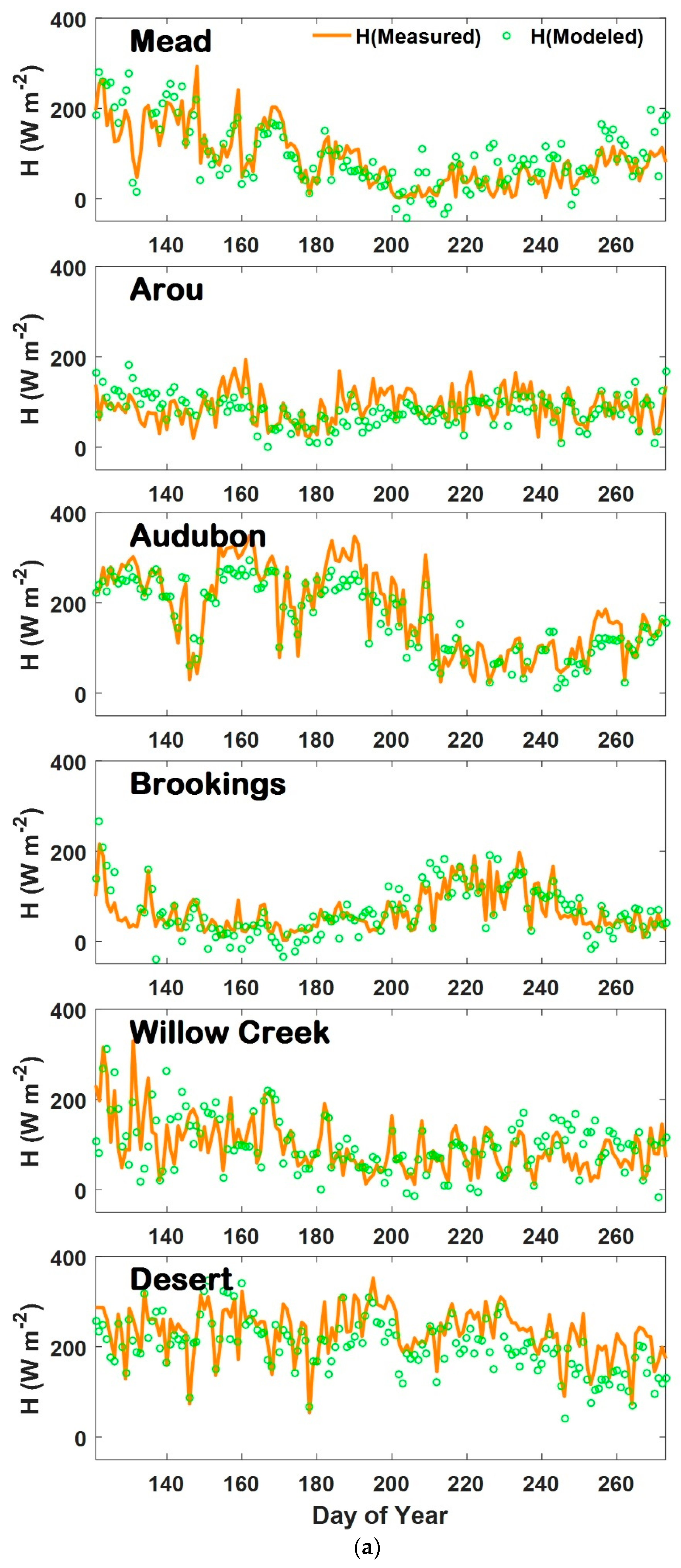
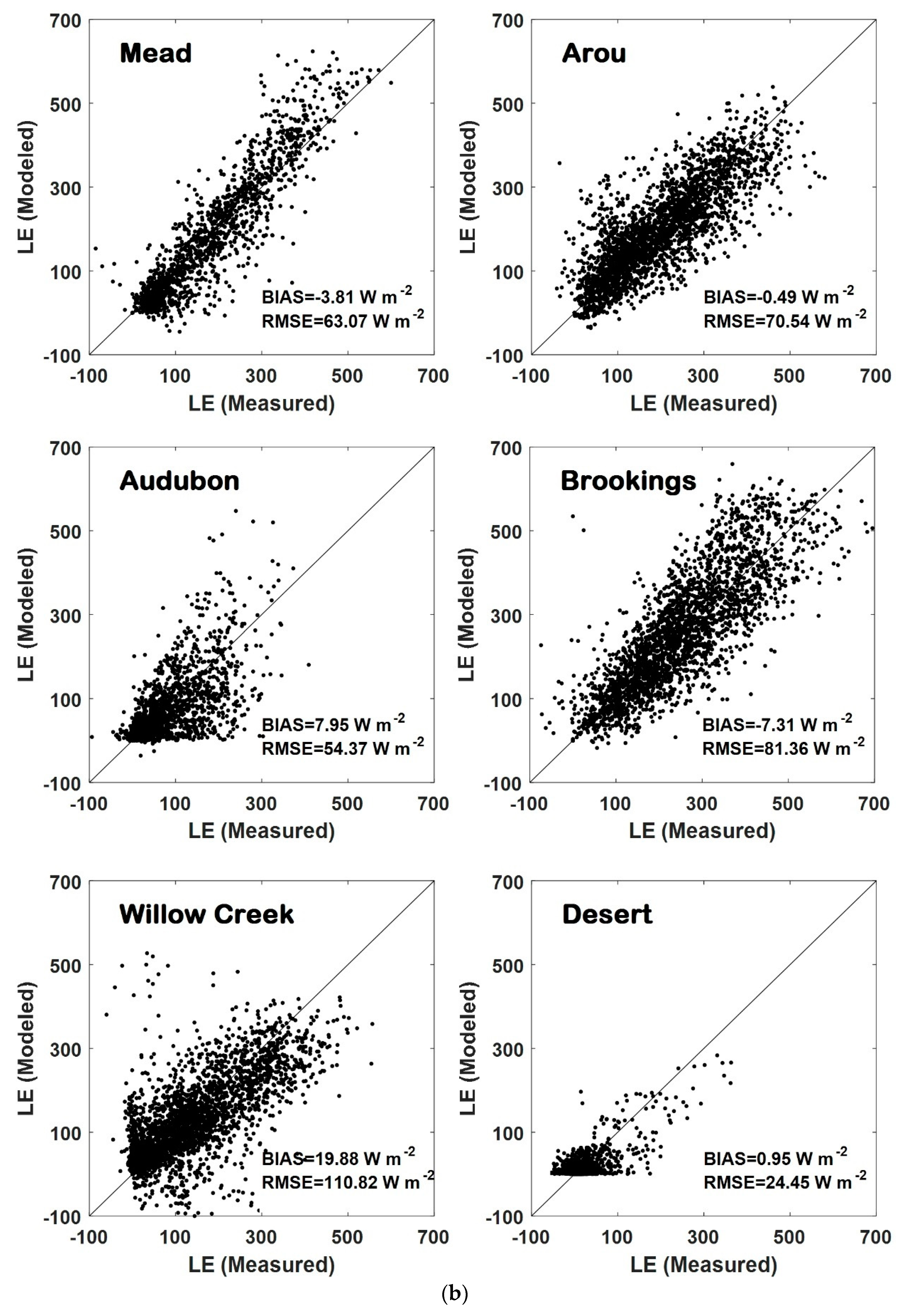
4.4. Sensible and Latent Heat Fluxes

Figure 3a,b shows the daytime-averaged (0900–1800 LT) sensible and latent heat flux estimates at the six sites during DOY 121–273. The estimated turbulent heat fluxes agree well with the ground measurements, implying that the WC-VDA approach can yield accurate turbulent heat flux estimates. However, the turbulent heat flux estimates degrade in wet periods (e.g., DOY 180–200 at the Brookings site and DOY 180–220 at the Willow Creek site). The Bias and RMSE of turbulent heat flux estimates from the WC-VDA approach at the Willow Creek site (higher precipitation and denser vegetation cover) are larger than those of Audubon and Desert sites (lower precipitation and sparser canopy cover) (Figure 4a,b). This is because drying rate is mainly controlled by the land surface state variable (i.e., LST) in dry and slightly vegetated sites. But, in wet and densely vegetated sites, evaporation is mainly influenced by the atmospheric state variables (i.e., air temperature and specific humidity) [59,60].
Figure 4a,b compares the half-hourly sensible and latent heat flux estimates from the WC-VDA method with the EC measurements at the six study sites. The estimated sensible and latent heat fluxes from the WC-VDA approach are in good consistency with the observations, and the scatterplots mainly fall around the 1:1 line. The WC-VDA model tends to overestimate (underestimate) H when it is smaller (larger) than 100 W·m−2. At the Mead, Audubon, and Brookings sites, the WC-VDA model tends to overestimate LE when it is larger than 200 W·m−2. Also, LE estimates are more sparsely distributed around the 1:1 line at the Willow Creek site (forest). This happens because performance of the WC-VDA degrades in heavily vegetated sites as LE is controlled dominantly by the atmospheric variables rather than the land surface processes. Similar results were also found in Xu et al. [36,39]. The misfits between the model estimates and observations are mainly due to the simplistic model assumptions (i.e., daily constant EF and monthly constant CHN), and measurement errors. Figure 4a,b also shows that LE estimates are more scattered around the 45-degree line than H. This is because the uncertainty of the H estimates comes from the errors in the CHN and LST estimates (see Equation (7)). LE is obtained by re-writing Equation (9) as follows: LE = EF/(1 − EF) × H. Hence, the uncertainty of LE values is due to the errors in the EF, CHN, and LST retrievals. More sources of errors increase scattering of LE estimates.
The Bias and RMSE of half-hourly turbulent heat flux estimates from the WC-VDA approach are summarized in Table 4a. For comparison, corresponding values from SC-VDA are also shown in the same table. For half-hourly sensible heat flux, the six-site-averaged RMSE from the WC-VDA approach is 59.51 W·m−2, which is 10.16% lower than the RMSE of 66.24 W·m−2 from SC-VDA. For latent heat flux, the six-site-averaged RMSE is 75.06 W·m−2 for the SC-VDA approach, and 67.44 W·m−2 for the WC-VDA approach. In a similar effort, the statistical indices for the daily H and LE estimates from the WC-VDA and SC-VDA approaches are shown in Table 4b. The six-site-averaged RMSE of estimated daily H and LE by SC-VDA are 44.58 W·m−2 and 45.32 W·m−2, respectively. The WC-VDA approach reduces the aforementioned RMSEs by 16.22% and 15.60%, implying that the WC-VDA method can absorb noise in the LST and micrometeorological forcing data, and does not allow measurement errors to propagate into EF and CHN, and consequently turbulent heat fluxes. Overall, the results in Table 4a,b show that WC-VDA outperforms SC-VDA.

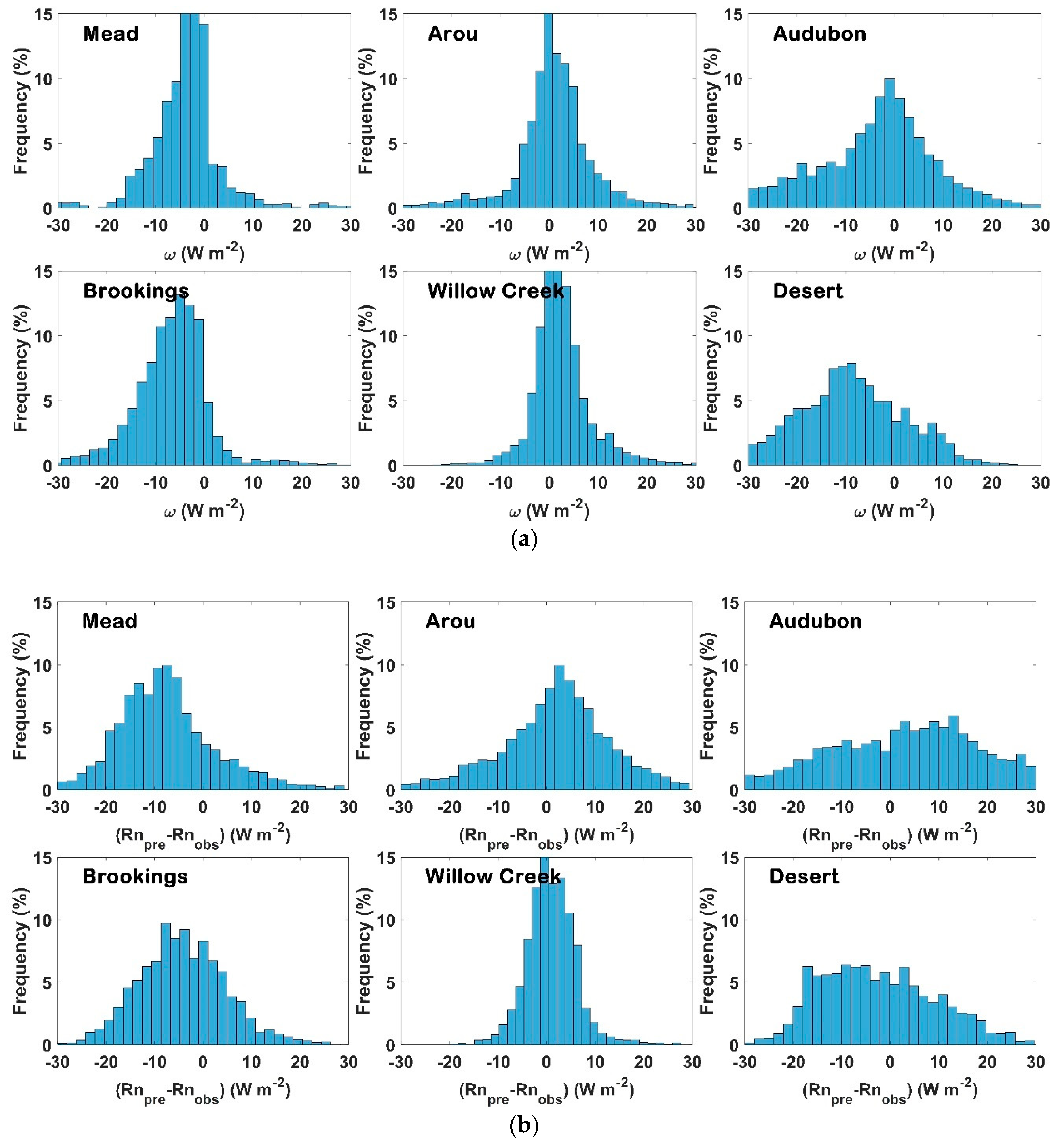
4.5. Model Error Analysis

Figure 5 shows time series of daily-averaged model error term (ω) and misfit between the predicted and observed net radiation (RnpreRnobs) from the WC-VDA approach at the six study sites. The misfit between the predicted and observed Rn is due to the difference between Tobs and Tpre, which itself is mainly because of the simplistic assumptions (i.e., constant soil thermal conductivity (P) and heat capacity (C) in the heat diffusion equation, monthly constant CHN, and daily constant EF). As shown in Figure 5, the estimated ω values show good consistency with the (RnpreRnobs). The model error term increases or decreases to capture the misfit between RnpreRnobs. For example, the model error term estimates at the Desert site with larger RnpreRnobs are higher than those at the Brookings and Willow Creek sites with smaller RnpreRnobs. The positive model error term at the Audubon (e.g., DOY 159–163) and Desert (e.g., DOY 196–200) sites is consistent with the positive (RnpreRnobs). For positive (RnpreRnobs), the model error term becomes positive to capture the overestimated Rn, thereby not allowing the errors in Rnpre to propagate into the sensible and latent heat fluxes. In contrast, when (RnpreRnobs) is negative (i.e., Rn is underestimated), the model error term becomes negative to balance the SEB equation. At some of the sites (e.g., Mead and Arou), there is a weaker consistency between ω and (RnpreRnobs). This is because the noise in the forcing data can affect the patterns of ω and weaken the consistency between ω and (RnpreRnobs).
To further evaluate the model robustness, the frequency histograms of the model error term (ω) and misfit between the predicted and observed net radiation (RnpreRnobs) are shown in Figure 6a,b, respectively. As illustrated, the frequency histograms of ω and (RnpreRnobs) are comparable, and they range from −30 W·m−2 to 30 W·m−2 at most of the sites. At the Mead, Brookings, and Desert sites, the distribution of (RnpreRnobs) is negatively-biased. Most likely this happens due to the inexact soil thermal properties (C and K), and the simplistic assumptions (e.g., constant daily EF and constant monthly CHN). Remarkably, the ω estimates at these sites have a negative bias to capture the negative misfit in (RnpreRnobs). At the Arou and Willow Creek sites, the frequency histograms of ω and RnpreRnobs are unbiased, and they both distribute almost symmetrically around 0 W·m−2. At the Audubon site, there is a weaker consistency between the frequency histograms of ω and RnpreRnobs. A possible explanation for this is because the model error term accounts for not only the structural model deficiencies (e.g., constant daily EF, constant monthly CHN, etc.), which leads to the underestimation or overestimation of Rn, but also the noise in the forcing variables, as well as parametric model errors. It is apparent that the noisy forcing and parametric model errors (pertains to having the inaccurate values of input parameters) can affect the distribution of ω and weaken the consistency between ω and (RnpreRnobs).
Two numerical experiments were conducted to examine whether the VDA approach with model uncertainty can capture errors in the meteorological input data. In the first (second) numerical experiment, positive (negative) noises with mean of 4 K (−4 K), 2 K (−2 K), 0.1 (−0.1), 30 W·m−2 (−30 W·m−2), and 1 m·s−1 (−1 m·s−1) and standard deviation of 2 K, 1 K, 0.02, 10 W·m−2, and 0.2 m s−1 were added respectively to the measured LST, air temperature, air humidity, incoming solar radiation, and wind speed at the Audubon site. The noises generated by the random Gaussian number generator were used to test the performance of the WC-VDA and SC-VDA approaches. Figure 7a shows the errors of H and LE estimates when the positively noised input variables were used in the WC-VDA and SC-VDA approaches. Analogously, Figure 7b indicates the errors of estimated H and LE values for negatively noised input variables. As shown, the WC-VDA approach can capture both the positive and negative noises in the input variables and reduces their effect on the H and LE estimates. In contrast, the SC-VDA approach is more susceptible to errors in the input data, which can be seen by higher errors in its H and LE estimates. As shown in Figure 7a,b, the time series of errors in the LE estimates from the WC-VDA and SC-VDA approaches indicates a significant increase from early August until mid-September (i.e., around DOYs 212–255). This happens because the Audubon site experiences high rainfall in this period. Performance of the VDA degrades in wet periods because LE is in Stage-I (energy-limited), is controlled mainly by the atmospheric variables, and the coupling between LST and EF weakens [59,60]. In this case, the retrieval of EF from LST becomes more uncertain, which ultimately causes large errors in the LE estimates. From mid-September towards the end of the modeling period, there is no rainfall and consequently the uncertainty of LE retrievals decreases.

5. Conclusions

In this study, the weak constraint-variational data assimilation (WC-VDA) method was tested at six sites with contrasting hydrological conditions. The key unknown parameters of the WC-VDA approach are neutral bulk transfer coefficient (CHN) and evaporative fraction (EF). The results showed that the neutral heat transfer coefficient (CHN) increases with the increase of leaf area index (LAI) although no information on vegetation phenology was used as input. The variations in evaporative fraction (EF) estimates are consistent with the drying and wetting events, while no precipitation or soil moisture observations were used in the WC-VDA approach. The estimated sensible and latent heat fluxes from the WC-VDA approach were validated with the eddy covariance (EC) observations at the six study sites, and compared to those of strong constraint-variational data assimilation (SC-VDA). For the WC-VDA scheme, the six-site-averaged root mean square errors (RMSEs) of sensible and latent heat fluxes are 59.51 W·m−2 and 67.44 W·m−2, respectively, which are 10.16% and 10.15% lower than those of SC-VDA. The findings indicated that the WC-VDA approach outperforms SC-VDA because the model error term can account for errors resulting from uncertainties in the micrometeorological input variables and inaccurate model parameters, as well as simplistic model parameterizations. This study evaluated the performance of the model error term in different hydrological and vegetative conditions. It was found that the model error term shows good consistency with the misfit between the predicted and observed net radiation (RnpreRnobs), implying that the model error term can capture the difference between the predicted and observed net radiation in various hydrological environments. This hinders the errors in the estimated net radiation values to transfer into the turbulent heat flux estimates. Finally, numerical experiments indicated that the WC-VDA approach can capture the synthetically added positive and negative noises to the nominal input variables and reduce their effect on the H and LE estimates.

Author Contributions

Methodology, S.M.B., T.X. and X.H.; data processing and analyze, X.H.; writing-original draft preparation, X.H.; writing-review and editing, T.X., S.M.B., C.N., T.A., S.L., K.W. K.M., and Y.Y.; Supervision, T.X.; project administration, T.X., S.M.B.; funding acquisition, T.X., S.M.B.

Funding

This work was funded by the National Natural Science Foundation of China (91647104 and 41671335), the United States Department of Agriculture-Natural Resources Conservation Service (USDA-NRCS) grant 69-3A75-17-54 and the United States Geological Service (USGS) grant 2017HI440B awarded to the University of Hawaii at Manoa.

Acknowledgments

The authors would like to thank all the scientists, engineers, and students who participated in HiWATER field campaigns. We thank two reviewers for their valuable comments that greatly improved the presentation of this paper.

Conflicts of Interest

The authors declare no conflict of interest.

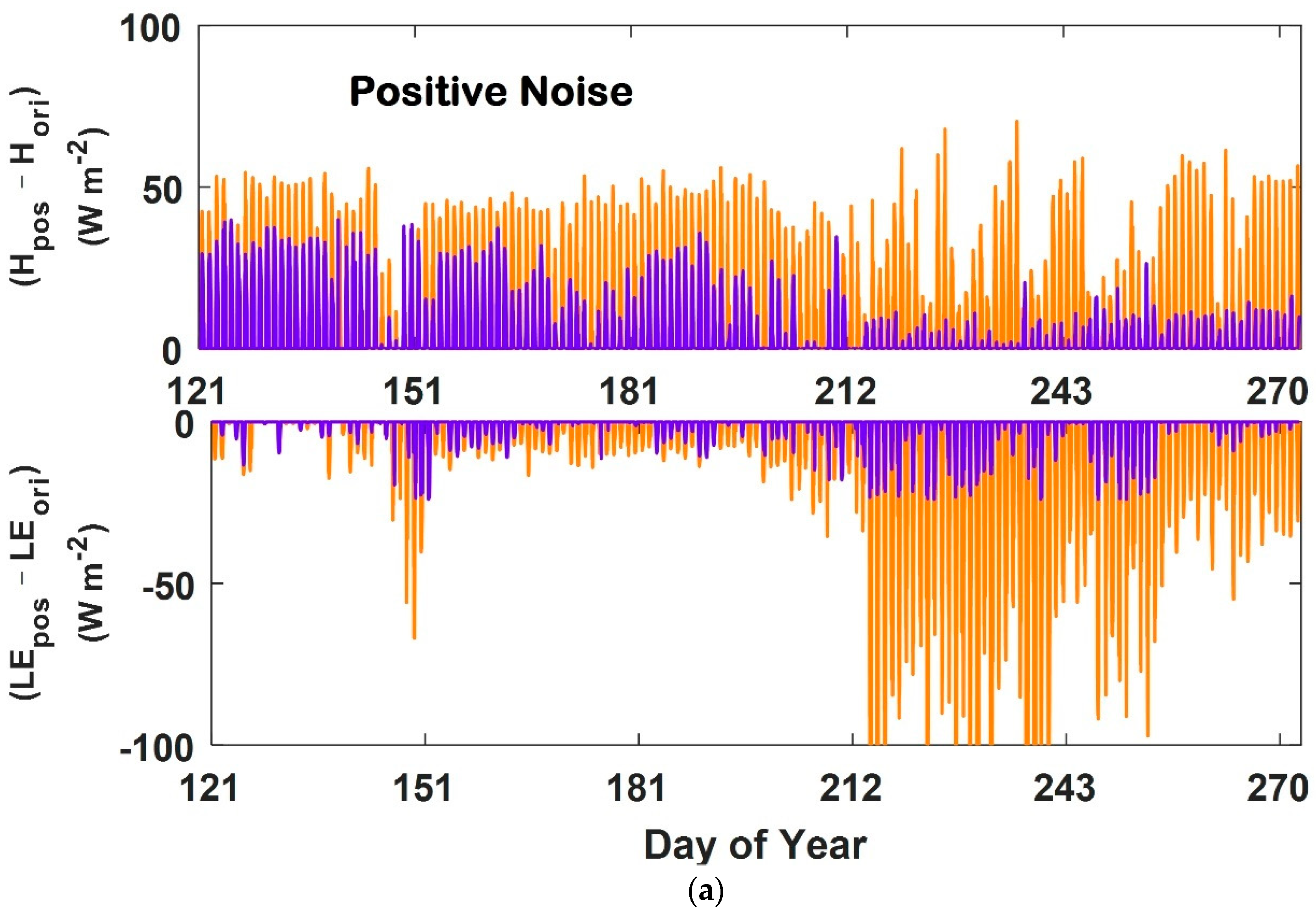
Appendix A. Difference between the 3D- and 4D-VDA Approaches

The principle of three dimensional variational data assimilation (3D-VDA) is to obtain an approximate solution by minimizing the cost function J,
J ( X ) = ( X X b ) T B 1 ( X X b ) + ( y H [ X ] ) T R 1 ( y H [ X ] ) ,
where X and Xb are the analysis model state and background model state, respectively, y is the vector of observations, H is the observation operator, and B and R are the covariance matrix of the background and observation errors, respectively.
Four dimensional variational data assimilation (4D-VDA) is an extension of 3D-VDA, which is used for time series of observations. The 4D-VDA method allows comparison of the model state with observations at the appropriate times. Over a specified assimilation period, the cost function J for the 4D-VDA can be shown as,
J ( X ) = ( X X b ) T B 1 ( X X b ) + i = 1 N ( y i H i [ X i ] ) T R i 1 ( y i H i [ X i ] ) ,
where yi and Xi are the observation and model state at time step i, respectively. Ri and Hi are the observation error covariance matrix and observation operator at time step i, respectively, and N is the total number of time steps in the assimilation period.
The 3D-VDA method collects observations during analysis time and does not require model integration. Therefore, the analysis increment does not evolve over time and requires less computing resources [61]. While, in the 4D-VDA method, all the observations in the assimilation period are incorporated into the model. The 4D-VDA method uses tangent linear and adjoint models to generate the propagation of analytical increments during the assimilation period, and requires more computational resources than 3D-VDA [62,63,64].

Appendix B. Euler-Lagrange Equations

The variational data assimilation (VDA) approach finds optimal values of R, EF, and ω iteratively, through the following steps: (1) integrate the heat diffusion equation (Equation (1)) forward in time using the boundary conditions at the top (Equation (2)) and bottom (Equation (3)) of the soil column, and the initial condition (Equation (4)), (2) integrate the adjoint model (Equation (A3)) backward in time using the final condition (Equation (A4)), and boundary conditions (Equations (A5) and (A6)), (3) update the parameters R, EF, and ω using Equations (A7)–(A9) , respectively, and (4) repeat steps (1)–(3) until convergence is reached.
λ t + ( K C ) 2 λ z 2 = 0 ,
λ ( z , τ 1 ) = 0 ,
λ z | z = 0 = ( C ) ( R T 1 ) K [ T ( 0 , t ) T O B S ( 0 , t ) ]
+ λ ( 0 , t ) p [ 4 ε g σ T 3 ( 0 , t ) + 1 1 EF ρ c p e R f ( R i ) U ] , λ z | z = l = 0
R = R 1 ( C ) ( B R 1 ) i = 1 N τ 0 τ 1 λ i ( 0 , t ) ρ c p e R U ( T ( 0 , t ) T a ) f ( R i ) 1 EF i d t ,
EF i = EF i 1 ( C ) ( B EF 1 ) τ 0 τ 1 λ i ( 0 , t ) ρ c p e R f ( R i ) U ( T ( 0 , t ) T a ) ( 1 EF i ) 2 d t ,
ω ( t ) = 1 c τ 0 τ 1 Q w 1 ( t , t ) λ ( 0 , t ) d t .

References

  1. Alfieri, J.G.; Blanken, P.D.; Smith, D.; Morgan, J. Concerning the measurement and magnitude of heat, watervapor, and carbon dioxide exchange from a semiarid grassland. J. Appl. Meteorol. Climatol. 2009, 48, 982–996. [Google Scholar] [CrossRef]
  2. Stephens, G.L.; Li, J.; Wild, M.; Clayson, C.A.; Loeb, N.; Kato, S.; L’Ecuyer, T.; Stackhouse, P.W.; Lebsock, M.; Andrews, T. An update on Earth’s energy balance in light of the latest global observations. Nat. Geosci. 2012, 5, 691–696. [Google Scholar] [CrossRef]
  3. Xu, T.; Guo, Z.; Liu, S.; He, X.; Meng, Y.; Xu, Z.; Xia, Y.; Xiao, J.; Zhang, Y.; Ma, Y.; et al. Evaluating different machine learning methods for upscaling evapotranspiration from flux towers to the regional scale. J. Geophys. Res. Atmos. 2018, 123, 8674–8690. [Google Scholar] [CrossRef]
  4. Norman, J.M.; Kustas, W.P.; Humes, K. Source approach for estimating soil and vegetation energy fluxes in observations of directional radiometric surface temperature. Agric. For. Meteorol. 1995, 77, 263–293. [Google Scholar] [CrossRef]
  5. Bastiaanssen, W.G.M.; Menenti, M.; Feddes, R.A.; Holtslag, A.A.M. A remote sensing surface energy balance algorithm for land (SEBAL): 1. Formulation. J. Hydrol. 1998, 212–213, 198–212. [Google Scholar] [CrossRef]
  6. Bastiaanssen, W.G.M.; Pelgrum, H.; Wang, J.; Ma, Y.; Moreno, J.F.; Roerink, G.J.; van der Wal, T. A remote sensing surface energy balance algorithm for land (SEBAL): 2. Validation. J. Hydrol. 1998, 212–213, 213–229. [Google Scholar] [CrossRef]
  7. Jiang, L.; Islam, S. Estimation of surface evaporation map over Southern Great Plain using remote sensing data. Water Resour. Res. 2001, 37, 329–340. [Google Scholar] [CrossRef]
  8. Su, Z. The Surface Energy Balance System (SEBS) for estimation of turbulent heat fluxes. Hydrol. Earth Syst. Sci. 2002, 6, 85–100. [Google Scholar] [CrossRef] [Green Version]
  9. Wang, K.C.; Dickinson, R.E. A review of global terrestrial evapotranspiration: Observation, modeling, climatology, and climatic variability. Rev. Geophys. 2012, 50. [Google Scholar] [CrossRef] [Green Version]
  10. Yao, Y.; Liang, S.; Li, X.; Chen, J.; Wang, K.; Jia, K.; Cheng, J.; Jiang, B.; Fisher, J.; Mu, Q.; et al. A satellite-based hybrid algorithm to determine the Priestley-Taylor parameter for global terrestrial latent heat flux estimation across multiple biomes. Remote Sens. Environ. 2015, 165, 216–233. [Google Scholar] [CrossRef]
  11. Song, L.S.; Kustas, W.P.; Liu, S.M.; Colaizzi, P.D.; Nieto, H.; Xu, Z.W.; Ma, Y.F.; Li, M.S.; Xu, T.R.; Agam, N.; et al. Applications of a thermal-based two-source energy balance model using Priestley-Taylor approach for surface temperature partitioning under advective conditions. J. Hydrol. 2016, 540, 574–587. [Google Scholar] [CrossRef] [Green Version]
  12. Fisher, J.B.; Melton, F.; Middleton, E.; Hain, C.; Anderson, M.; Allen, R.; McCabe, M.; Hook, S.; Baldocchi, D.; Townsend, P.A.; et al. The Future of Evapotranspiration: Global requirements for ecosystem functioning, carbon and climate feedbacks, agricultural management, and water resources. Water Resour. Res. 2017, 53, 2618–2626. [Google Scholar] [CrossRef]
  13. Ma, Y.; Liu, S.; Song, L.; Xu, Z.; Liu, Y.; Xu, T.; Zhu, T. Estimation of daily evapotranspiration and irrigation water efficiency at a Landsat-like scale for an arid irrigation area using multi-source remote sensing data. Remote Sens. Environ. 2018, 216, 715–734. [Google Scholar] [CrossRef]
  14. Bateni, S.; Entekhabi, D. Surface heat flux estimation with the ensemble Kalman smoother: Joint estimation of state and parameters. Water Resour. Res. 2012, 48, W08521. [Google Scholar] [CrossRef]
  15. Jiang, L.; Islam, S. An intercomparison of regional latent heat flux estimation using remote sensing data. Int. J. Remote Sens. 2003, 24, 2221–2236. [Google Scholar] [CrossRef]
  16. Nishida, K.; Nemani, R.R.; Glassy, J.M.; Running, S.W. Development of an evapotranspiration Index from Aqua/MODIS for monitoring surface moisture status. IEEE Geosci. Remote Sens. 2003, 41, 493–500. [Google Scholar] [CrossRef]
  17. Wang, K.; Li, Z.; Cribb, M. Estimating of evaporative fraction from a combination of day and night land surface temperature and NDVI: A new method to determine the Priestley-Taylor parameter. Remote Sens. Environ. 2006, 102, 293–305. [Google Scholar] [CrossRef]
  18. Tang, R.; Li, Z.L.; Tang, B. An application of the Ts-VI triangle method with enhanced edges determination for evapotranspiration estimation from MODIS data in arid and semi-arid regions: Implementation and validation. Remote Sens. Environ. 2010, 114, 540–551. [Google Scholar] [CrossRef]
  19. Sun, L.; Liang, S.; Yuan, W.; Chen, Z. Improving a Penman-Monteith evapotranspiration model by incorporating soil moisture control on soil evaporation in semiarid areas. Int. J. Digit. Earth 2013, 6, 134–156. [Google Scholar] [CrossRef]
  20. Zhu, W.; Jia, S.; Lv, A. A universal Ts-VI triangle method for the continuous retrieval of evaporative fraction from MODIS products. J. Geophys. Res. Atmos. 2017, 122, 10206–10227. [Google Scholar] [CrossRef]
  21. Liu, S.M.; Hu, G.; Lu, L. Estimation of regional evapotranspiration by TM/ETM+ data over heterogeneous surfaces. Photogramm. Eng. Remote Sens. 2007, 73, 1169–1178. [Google Scholar] [CrossRef]
  22. Jia, L.; Xi, G.; Liu, S.; Huang, C.; Yan, Y.; Liu, G. Regional estimation of daily to annual regional evapotranspiration with MODIS data in the Yellow River Delta wetland. Hydrol. Earth Syst. Sci. 2009, 13, 1775–1787. [Google Scholar] [CrossRef]
  23. Mallick, K.; Jarvis, A.J.; Fisher, J.B.; Tu, K.P.; Boegh, E.; Niyogi, D. Latent heat flux and canopy conductance based on Penman-Monteith, Priestly-Taylor equation, and Bouchets complementary hypothesis. J. Hydrometeorol. 2013, 14, 419–442. [Google Scholar] [CrossRef]
  24. Mallick, K.; Jarvis, A.J.; Boegh, E.; Fisher, J.B.; Drewry, D.T.; Tu, K.P.; Hook, S.J.; Hulley, G.; Ardö, J.; Beringer, J.; et al. A surface temperature initiated closure (STIC) for surface energy balance fluxes. Remote Sens. Environ. 2014, 141, 243–261. [Google Scholar] [CrossRef]
  25. Peters-Lidard, C.D.; Kumar, S.V.; Mocko, D.M.; Tian, Y. Estimating evapotranspiration with land data assimilation systems, hydrological processes. Hydrol. Processes 2011, 25, 3979–3992. [Google Scholar] [CrossRef]
  26. Xu, T.R.; Liu, S.M.; Liang, S.; Qin, J. Improving predictions of water and heat fluxes by assimilating MODIS land surface temperature products into common land model. J. Hydrometeorol. 2011, 12, 227–244. [Google Scholar] [CrossRef]
  27. Xu, T.R.; Liang, S.; Liu, S. Estimating turbulent fluxes through assimilation of geostationary operational environmental satellites data using ensemble Kalman filter. J. Geophys. Res. 2011, 116, D09109. [Google Scholar] [CrossRef]
  28. Xu, T.R.; Liu, S.M.; Xu, Z.W.; Liang, S.; Xu, L. A dual-pass data assimilation scheme for estimating surface fluxes with FY3A-VIRR land surface temperature. Sci. China Earth Sci. 2015, 58, 211–230. [Google Scholar] [CrossRef]
  29. Xia, Y.; Sheffield, J.S.; Ek, M.B.; Dong, J.; Chaney, N.; Wei, H.; Meng, J.; Wood, E.F. Evaluation of multi-model simulated soil moisture in NLDAS-2. J. Hydrol. 2014, 512, 107–125. [Google Scholar] [CrossRef]
  30. Xia, Y.; Ek, M.; Mocko, D.; Peters-Lidard, C.; Sheffield, J.; Dong, J.; Wood, E. Uncertainties, correlations, and optimal blends of drought indices from the NLDAS multiple land surface model ensemble. J. Hydrometeor. 2014. [Google Scholar] [CrossRef]
  31. Carrera, M.; Belair, S.; Bilodeau, B. The Canadian Land Data Assimilation System (CaLDAS): Description and synthetic evaluation study. J. Hydrometeor. 2015, 16, 1293–1314. [Google Scholar] [CrossRef]
  32. Crow, W.T.; Kustas, W.P. Utility of assimilating surface radiometric temperature observations for evaporative fraction and heat transfer coefficient retrieval. Bound. Layer Meteorol. 2005, 115, 105–130. [Google Scholar] [CrossRef]
  33. Sini, F.; Boni, G.; Caparrini, F.; Entekhabi, D. Estimation of large-scale evaporation fields based on assimilation of remotely sensed land temperature. Water Resour. Res. 2008, 44, W06410. [Google Scholar] [CrossRef]
  34. Bateni, S.M.; Liang, S. Estimating surface energy fluxes using a dual-source data assimilation approach adjoined to the heat diffusion equation. J. Geophys. Res. 2012, 117, D17118. [Google Scholar] [CrossRef]
  35. Bateni, S.M.; Entekhabi, D.; Jeng, D.S. Variational assimilation of land surface temperature and the estimation of surface energy balance components. J. Hydrol. 2013, 481, 143–156. [Google Scholar] [CrossRef]
  36. Xu, T.R.; Bateni, S.M.; Liang, S.; Entekhabi, D.; Mao, K.B. Estimation of surface turbulent heat fluxes via variational assimilation of sequences of land surface temperatures from Geostationary Operational Environmental Satellites. J. Geophys. Res. 2014, 119, 10780–10798. [Google Scholar] [CrossRef]
  37. Xu, T.R.; Bateni, S.M.; Liang, S. Estimating turbulent heat fluxes with a weak-constraint data assimilation scheme: A case study (HiWATER-MUSOEXE). IEEE Geosci. Remote Sens. 2015, 12, 68–72. [Google Scholar]
  38. Xu, T.R.; Bateni, S.M.; Margulis, S.A.; Song, L.; Liu, S.M.; Xu, Z.W. Partitioning Evapotranspiration into Soil Evaporation and Canopy Transpiration via a Two-Source Variational Data Assimilation System. J. Hydrometeorol. 2016, 17, 2353–2370. [Google Scholar] [CrossRef]
  39. Xu, T.; Bateni, S.M.; Neale, C.M.U.; Auligne, T.; Liu, S. Estimation of turbulent heat fluxes by assimilation of land surface temperature observations from GOES satellites into an ensemble Kalman smoother framework. J. Geophys. Res. Atmos. 2018, 123, 2409–2423. [Google Scholar] [CrossRef]
  40. Abdolghafoorian, A.; Farhadi, L.; Bateni, S.M.; Margulis, S.; Xu, T.R. Characterizing the effect of vegetation dynamics on the bulk heat transfer coefficient to improve variational estimation of surface turbulent fluxes. J. Hydrometeorol. 2017, 18, 321–333. [Google Scholar] [CrossRef]
  41. Hu, Z.; Islam, S. Prediction of ground temperature and soil moisture content by the force–restore method. Water Resour. Res. 1995, 31, 2531–2539. [Google Scholar] [CrossRef]
  42. Bateni, S.M.; Entekhabi, D.; Castelli, F. Mapping evaporation and estimation of surface control of evaporation using remotely sensed land surface temperature from a constellation of satellites. Water Resour. Res. 2013, 49, 950–968. [Google Scholar] [CrossRef] [Green Version]
  43. Gentine, P.; Entekhabi, D.; Chehbouni, A.; Boulet, G.; Duchemin, B. Analysis of evaporative fraction diurnal behaviour. Agric. For. Meteorol. 2007, 143, 13–29. [Google Scholar] [CrossRef] [Green Version]
  44. Reichle, R.H. Data assimilation methods in the earth sciences. Adv. Water Resour. 2008, 31, 1411–1418. [Google Scholar] [CrossRef]
  45. Margulis, S.; Entekhabi, D. Variational assimilation of surface temperature and micrometeorology into a model of the atmospheric boundary layer and land surface. Mon. Weather Rev. 2003, 131, 1272–1288. [Google Scholar] [CrossRef]
  46. Rodgers, C. Inverse Methods for Atmospheric Sounding; World Scientific: Singapore, 2000. [Google Scholar]
  47. Tremolet, Y. Accounting for an imperfect model in 4d-var. Quart. J. R. Meteorol. Soc. 2006, 132, 2483–2504. [Google Scholar] [CrossRef]
  48. Baldocchi, D.; Falge, E.; Gu, L.H.; Olson, R. FLUXNET: A new tool to study the temporal and spatial variability of ecosystem-scale carbon dioxide, water vapor, and energy flux densities. Bull. Am. Meteorol. Soc. 2001, 82, 2415–2434. [Google Scholar] [CrossRef]
  49. Liu, S.M.; Xu, Z.W.; Wang, W.Z.; Bai, J.; Jia, Z.; Zhu, M.; Wang, J.M. A comparison of eddy-covariance and large aperture scintillometer measurements with respect to the energy balance closure problem. Hydrol. Earth Syst. Sci. 2011, 15, 1291–1306. [Google Scholar] [CrossRef] [Green Version]
  50. Li, X.; Cheng, G.D.; Liu, S.M.; Xiao, Q.; Ma, M.G.; Jin, R.; Che, T.; Liu, Q.H.; Wang, W.Z.; Qi, Y.; et al. Heihe Watershed Allied Telemetry Experimental Research (HiWATER): Scientific objectives and experimental design. Bull. Am. Meteorol. Soc. 2013, 94, 1145–1160. [Google Scholar] [CrossRef]
  51. Xiao, Z.; Liang, S.; Wang, J.; Chen, P.; Yin, X.; Zhang, L.; Song, J. Use of general regression neural networks for generating the GLASS leaf area index product from time-series MODIS surface reflectance. IEEE Trans. Geosci. Remote Sens. 2013, 52, 209–223. [Google Scholar] [CrossRef]
  52. Xiao, Z.; Liang, S.; Wang, J.; Xiang, Y.; Zhao, X.; Song, J. Long-Time-Series Global Land Surface Satellite Leaf Area Index Product Derived From MODIS and AVHRR Surface Reflectance. IEEE Trans. Geosci. Remote Sens. 2016, 54, 5301–5318. [Google Scholar] [CrossRef]
  53. Chen, S.X. Thermal conductivity of sands. Heat Mass Transf. 2008, 44, 1241–1246. [Google Scholar] [CrossRef]
  54. Farouki, O.T. Thermal Properties of Soils; TransTech: Clausthal-Zellerfeld, Germany, 1986. [Google Scholar]
  55. Usowicz, B.; Lipiec, J.; Marczewski, W.; Ferrero, A. Thermal conductivity modeling of terrestrial soil media—A comparative study. Planet. Space Sci. 2006, 54, 1086–1095. [Google Scholar] [CrossRef]
  56. Song, X.; Liu, F.; Zhang, G.; Li, D.; Zhao, Y. Estimation of soil texture at a regional scale using local soil-landscape models. Soil Sci. 2016, 181, 435–445. [Google Scholar] [CrossRef]
  57. Brutsaert, W. Heat and mass transfer to and from surfaces with dense vegetation or similar permeable roughness. Bound. Layer Meteorol. 1979, 16, 365–388. [Google Scholar] [CrossRef]
  58. Duynkerke, P.G. The roughness length for heat and other vegetation parameters for a surface of short grass. J. Appl. Meteorol. 1992, 31, 579–586. [Google Scholar] [CrossRef]
  59. Shokri, N.; Lehmann, P.; Vontobel, P.; Or, D. Drying front and water content dynamics during evaporation from sand delineated by neutron radiography. Water Resour. Res. 2008, 44, W06418. [Google Scholar] [CrossRef]
  60. Shokri, N.; Lehmann, P.; Or, D. Characteristics of evaporation from partially wettable porous media. Water Resour. Res. 2008, 45, W02415. [Google Scholar] [CrossRef]
  61. Mazzarella, V.; Maiello, I.; Capozzi, V.; Budillon, G.; Ferretti, R. Comparison between 3D-Var and 4D-Var data assimilation methods for the simulation of a heavy rainfall case in central Italy. Adv. Sci. Res. 2017, 14, 271–278. [Google Scholar] [CrossRef] [Green Version]
  62. Errico, R.M. What is an adjoint method? Bull. Am. Meteorol. Soc. 1997, 78, 2577–2591. [Google Scholar] [CrossRef]
  63. Errico, R.M.; Reader, K.D. An examination of the accuracy of the linearization of a mesoscale model with moist physics. Q. J. R. Meteorol. Soc. 1999, 125, 169–195. [Google Scholar] [CrossRef]
  64. Errico, R.M.; Vukicevic, T.; Reader, K. Examination of the accuracy of a tangent linear model. Tellus 1993, 45A, 462–477. [Google Scholar] [CrossRef]
Figure 1. Time series of evaporative fraction (EF) observations and estimates from the weak constraint-variational data assimilation (WC-VDA) approach at the six study sites.
Remotesensing 10 01994 g001
Figure 2. Half-hourly estimated land surface temperature (LST) values from weak constraint-variational data assimilation (WC-VDA) versus observations for the six study sites.
Remotesensing 10 01994 g002
Figure 3. (a) Time series of observed (open circles) and estimated (lines) daytime-averaged sensible heat flux (H) from the weak constraint-variational data assimilation (WC-VDA) approach at the six experimental sites. (b) Time series of observed (open circles) and estimated (lines) daytime-averaged latent heat flux (LE) estimates from the WC-VDA approach at the six experimental sites.
Remotesensing 10 01994 g003aRemotesensing 10 01994 g003b
Figure 4. (a) Scatterplot of half-hourly sensible heat flux estimates from the weak constraint-variational data assimilation (WC-VDA) approach versus measurements at the six sites for DOY 121–273. (b) Scatterplot of half-hourly latent heat flux estimates from the WC-VDA approach versus measurements at the six sites for DOY 121–273.
Remotesensing 10 01994 g004aRemotesensing 10 01994 g004b
Figure 5. Time series of model error term estimates (left column) and misfit between daily estimated and observed net radiation (right column) from the weak constraint-variational data assimilation (WC-VDA) scheme in the six experimental sites.
Remotesensing 10 01994 g005
Figure 6. (a) Frequency histogram of the model error term (ω) at the six experimental sites (blue bars). (b) Frequency histogram of the difference between estimated and observed net radiation (RnpreRnobs) at the six experimental sites (blue bars).
Remotesensing 10 01994 g006
Figure 7. (a) Time series of errors in the sensible (H) and latent (LE) estimates (i.e., Hpositive noiseHoriginal & LEpositive noise − LEoriginal) from the weak constraint-variational data assimilation (WC-VDA) (purple lines) and strong constraint-variational data assimilation (SC-VDA) (orange lines) approaches at the Audubon sites. Horiginal and LEoriginal are obtained by using the nominal input data in the WC-VDA and SC-VDA approaches. Hpositive noise and LEpositive noise are estimated by using the positively noised input data in the WC-VDA and SC-VDA approaches. (b) Time series of errors in the H and LE estimates (i.e., Hnegative noiseHoriginal & LEnegative noise − LEoriginal) from the WC-VDA (purple lines) and SC-VDA (orange lines) approaches. Horiginal and LEoriginal are obtained by using the nominal input data in the WC-VDA and SC-VDA approaches. Hpositive noise and LEpositive noise are estimated by using the negatively noised input data in the WC-VDA and SC-VDA approaches.
Remotesensing 10 01994 g007aRemotesensing 10 01994 g007b
Table 1. Characteristics of the six study sites.
SiteLocationLand CoverLAIfcSMElevation (m)
Mead41.18N, 96.44WCropland1.750.530.25363
Arou38.04N, 100.46EGrassland2.530.720.343033
Audubon31.59N, 110.51WGrassland0.390.170.071469
Brookings44.34N, 96.83WGrassland2.240.670.45510
Willow Creek45.80N, 90.08WForest4.80.910.30520
Desert42.11N, 100.99EBarren land000.011000
LAI, fc, and SM represent the mean leaf area index (m2·m−2), vegetation cover fraction (-), and soil moisture (m3·m−3) over the growing period (DOY 121–273), respectively.
Table 2. Neutral bulk heat transfer coefficient (CHN) estimates from the weak constraint-variational data assimilation (WC-VDA) model, and corresponding leaf area index (LAI) values.
Site 121–151152–181182–212213–243244–273
MeadCHN0.22 × 10−20.40 × 10−21.22 × 10−21.48 × 10−20.78 × 10−2
LAI0.771.282.422.701.54
ArouCHN0.12 × 10−20.46 × 10−23.35 × 10−25.12 × 10−21.98 × 10−2
LAI0.461.773.794.222.42
AudubonCHN0.31 × 10−20.35 × 10−20.42 × 10−20.31 × 10−20.25 × 10−2
LAI0.230.300.350.540.53
BrookingsCHN0.72 × 10−21.54 × 10−23.12 × 10−21.55 × 10−20.62 × 10−2
LAI1.302.372.852.741.94
Willow CreekCHN6.33 × 10−27.45 × 10−28.61 × 10−214.35 × 10−28.13 × 10−2
LAI2.645.355.885.734.40
DesertCHN0.13 × 10−30.14 × 10−30.18 × 10−30.19 × 10−30.12 × 10−3
LAI00000
Table 3. Bias and Root Mean Square Error (RMSE) of half-hourly land surface temperature (LST) estimates from the weak constraint-variational data assimilation (WC-VDA) and strong constraint-variational data assimilation (SC-VDA) approaches at the six experimental sites.
Bias (K)RMSE (K)
Study SitesWC-VDASC-VDAWC-VDA SC-VDA
Mead0.82−1.231.551.71
Arou0.300.51.972.07
Audubon0.060.232.372.75
Brookings−0.76−0.861.711.72
Willow Creek0.210.560.991.06
Desert−0.41−0.922.052.53
Six-sites-average0.04−0.291.771.97
Table 4. a. Statistical indices of half-hourly sensible (H) and latent (LE) estimates from the weak constraint-variational data assimilation (WC-VDA) and strong constraint-variational data assimilation (SC-VDA) approaches at the six experimental sites. b. Statistical indices of daily H and LE estimates from the WC-VDA and SC-VDA approaches at the six experimental sites.
a
Study SiteMethodH (W·m−2)LE (W·m−2)
BiasRMSEBiasRMSE
MeadWC-VDA (SC-VDA)8.73 (10.21)64.60 (69.25)−3.81 (−8.65)63.07 (75.55)
ArouWC-VDA (SC-VDA)−11.64 (−15.75)52.28 (55.63)−0.49 (5.32)70.54 (79.88)
AudubonWC-VDA (SC-VDA)16.25 (20.21)56.44 (67.82)7.95 (12.19)54.37 (57.55)
BrookingsWC-VDA (SC-VDA)4.77 (10.88)42.72 (45.35)−7.31 (−11.60)81.36 (83.86)
Willow CreekWC-VDA (SC-VDA)7.67 (22.17)86.74 (91.18)19.88 (32.49)110.82 (125.60)
DesertWC-VDA (SC-VDA)7.08 (12.68)54.30 (68.21)0.95 (1.25)24.45 (27.91)
b
Study SiteMethodH (W·m−2)LE (W·m−2)
BiasRMSEBiasRMSE
MeadWC-VDA (SC-VDA)5.32 (9.45)40.89 (43.28)−3.05 (−7.51)40.75 (47.62)
ArouWC-VDA (SC-VDA)−0.37 (−3.43)31.56 (38.69)3.56 (17.74)32.71 (50.58)
AudubonWC-VDA (SC-VDA)12.04 (16.15)31.95 (42.09)0.51 (−7.32)28.86 (22.98)
BrookingsWC-VDA (SC-VDA)2.50 (8.82)33.91 (36.54)−13.13 (−17.61)60.52 (64.87)
Willow CreekWC-VDA (SC-VDA)5.38 (19.88)52.46 (57.23)19.12 (25.76)56.59 (73.18)
DesertWC-VDA (SC-VDA)7.51 (12.69)33.30 (49.64)0.43 (0.97)10.04 (12.71)

