Article

Partitioning of Terrain Features Based on Roughness

College of Urban and Environmental Sciences, Northwest University, No. 1 Xuefu Street, Chang’an District, Xi’an 710127, China
*
Author to whom correspondence should be addressed.
Remote Sens. 2018, 10(12), 1985; https://doi.org/10.3390/rs10121985
Submission received: 23 September 2018 / Revised: 5 December 2018 / Accepted: 5 December 2018 / Published: 7 December 2018

Abstract

:
Surface roughness is a key parameter that reflects topographic characteristics and influences surface processes, and characterization of surface roughness is a fundamental problem in geoscience. In recent years, although there have been basic studies on roughness, few studies have compared the concept and quantification of roughness, and there have been few studies that have evaluated the ability of partition terrain features. Based on 1″ resolution Shuttle Radar Topography Mission (SRTM) data and previous studies, we selected the Qinba Mountain region of China and its adjacent areas as our study area, and used 13 different roughness algorithms to extract roughness in this study. Using spatial patterns and statistical distributions, the results were analyzed, and the best algorithm suited to partitioning terrain features was selected. We then evaluated the ability of the algorithm to distinguish the terrain morphology. The results showed the following: (1) The 13 algorithms were able to be classified into four types, that is, gradient (SLOPE), relief (root mean squared height, RMSH), local vector (directional cosine eigenvalue, DCE) and power-spectral (two-dimensional continuous wavelet transform, 2D CWT). (2) The SLOPE and RMSH algorithms were better able to express and distinguish terrain, as they were able to macroscopically distinguish between four types of terrain in the study areas. Based on power-spectral methods, 2D CWT had the same discrimination ability as the first two methods following a normalization transform, whereas the DCE method had a general effect and could only distinguish two types of terrain. (3) Different roughness algorithms had their own applicability for different terrain areas and application directions.

1. Introduction

The basic definition of roughness is the degree of deviation between a real surface and an ideal surface (geoid) in the vertical direction. If the deviations are large, the surface is rough. If the deviations are small, the surface is smooth [1]. The concept of roughness in the literature has been used in three ways: For local variation in surface elevation [2,3], for the influence of topography on surface fluid (flow resistance or roughness height, a property of a flow) [4,5,6], and for random variation in soil surface elevation [7]. These three aspects emphasize the structural characteristics of the topography, the relationship between the surface and airflow or water flow, and the influence of the surface microrelief on runoff at the subpixel level. This article primarily discusses the first aspect.
All surface material movements, such as slope runoff, rivers, wind and sand flows, air currents on vegetation or buildings, and ocean currents, are inevitably affected by rough land surfaces: At the same time, new rough surfaces also evolve over the course of surface movement [8]. The roughness of the surface can effectively reflect the terrain characteristics and degree of erosion. Therefore, surface roughness is an important parameter that is used to identify the individual characteristics of erosive terrain and to analyze the relationship between roughness and surface processes [3]. Accordingly, many scholars have studied land surface roughness.
Hobson was the first to discuss the concept and algorithms of roughness, and summarizes the roughness algorithm as three kinds: The area ratio, the statistical distribution irregularity of the elevation, and the aggregation degree of the unit direction vector [9]. Hoffman specified the various characteristics that the roughness algorithm should have (effect, property, meaning) [10]. Using 60 data sets, Shepard et al. analyzed seven quantitative metrics of roughness and discussed the scale-dependent problems of roughness [2]. Based on Light Detection And Ranging (LiDAR ) topographic data, McKean, Roering, and Glenn et al. and Booth et al. analyzed landslide location distributions and characteristics using different roughness calculation methods [11,12,13]. Grohmann evaluated six roughness algorithms at different spatial scales and resolutions [3]. Pommerol et al. compared and evaluated the degree of roughness by calculating the slope distribution of two types of topography of three planets [14]. Berti et al. used mathematical artificial surfaces and natural surfaces to compare and analyze 10 roughness algorithms and explored the ability of the different algorithms to identify and predict active landslides for automatic mapping [15]. Lane and Smith comprehensively analyzed the concept, quantity and application of roughness [8,16]. However, the main research gaps are as follows: (1) There is a lack of comparison between the concepts and results of the different algorithms, so it is not clear which algorithms are better; (2) there are relatively few studies on the ability of the various algorithms to distinguish rough terrain of large regions, which has profound research significance.
Based on these problems, we used the Qinba Mountain region and its adjacent areas of China as the study area in our research, where the relief is obvious. First, various algorithms were systemically arranged, and the slope [17] and topographic relief [18] were included in the index of roughness. In addition, we calculated a variety of thematic roughness layers in the study area. Second, through analysis of the statistical distribution of the spatial patterns, we determined the optimal algorithm for the partitioning of terrain features based on roughness. Finally, we analyzed and evaluated the ability of this optimal algorithm on the terrain partition and quantization of the terrain shape. This study is of high theoretical significance for classifying surface morphology and analyzing the relationship between roughness and surface processes.

2. Materials and Methods

2.1. Study Area

The study area was located in a transitional zone between central and western China at a latitude and longitude range of 105°13′40″ E–110°44′38″ E and 30°5′38″ N–35°53′49″ N respectively. The study area covered an area of 347,500 km2 and spanned Shaanxi Province, Gansu Province, Ningxia Hui Autonomous Region, Sichuan Province, Chongqing City, Hubei Province, Henan Province, and Shanxi Province (Figure 1). The study area was located on the second topographic terrace. The topography in the study area is complex and diverse, and the terrain is quite undulating. Loess hills and platforms, stony hillsides, alluvial plains, and other types of topography are distributed from north to south in the study area. The study area is a typical area for studying the partitioning of terrain features by extracting roughness.

2.2. Basic Research Data

The raw data for extracting roughness in this manuscript were 1” Shuttle Radar Topographic Mission (SRTM) data downloaded from the United States Geological Survey (USGS) website (https://e4ftl01.cr.usgs.gov/SRTM/) using WGS-84 geographic coordinates and HGT as the data format. Before extracting roughness, the data were first converted to an ArcGrid format, and then a 3 × 3 window Gaussian low-pass filter algorithm was used to preprocess the digital elevation model (DEM) to filter the noise on the surface of the DEM. Finally, the projection was converted to Universal Transverse Mercator (UTM) coordinates with a central meridian of 108° E.

3. Research Methods and Models

3.1. Introduction of the Algorithms

This paper uses the surface roughness to express the topographical structural features (local variation of surface elevation) as the starting point of the study. The algorithm for quantifying surface roughness was compiled by previous research (key characteristics of methods are shown in Table 1). Considering that the calculation results are quantitative expressions of roughness, the calculation methods described below are collectively referred to as algorithms.
(1)
Slope (SLOPE), defined as the angle between the tangent plane and horizontal plane at any point on the surface, is one of the most important surface morphological indicators. By calculating the elevation gradient, the Evans algorithm [19] was adopted to calculate the slope in this study.
(2)
The local elevation range (RANGE), which is measured as the height deviation within a certain amplitude of distances from the ground [5], is the most common algorithm of topographic relief.
(3)
The area ratio (AR) is a commonly used method to measure surface roughness, which is calculated as the ratio of the actual area to the projected area of the surface [3]. In a moving window, the area ratio of each pixel is calculated as the reciprocal of the cosine value of the slope. This principle is based on the triangular relationship between the inclined slope and horizontal projection surface.
(4)
The root mean squared height (RMSH) is the most commonly used algorithm to calculate and evaluate roughness, and its parameters are also easy to obtain. RMSH expresses surface roughness as the standard deviation of the elevation of a set of geographic data (Shepard et al., 2001) [2].
(5)
The root mean squared deviation (RMSD) is the height difference between two points of a constant lag distance in the local range. In the roughness calculation, the RMSD is the mean square deviation of the height difference between an edge pixel and center pixel in a moving window [2].
(6)
The root mean squared slope (RMSS) is another method for calculating roughness based on the mean square root and is defined as the ratio of the mean square deviation of the local elevation to the horizontal distance [2].
(7)
The standard deviation of slope (SDS) calculates the standard deviation of the slope and quantifies the roughness of the surface according to the complexity of the changes in the local surface slope [20].
(8)
The absolute slope (AS) is similar to the root mean square slope. Both are essentially a deformation of SLOPE [21]. This algorithm can reduce the influence of outliers on the RMSS.
(9)
Vector dispersion (VD) can be effectively used to quantify surface roughness based on the spatial variability of the unit direction vector (variability in slope and aspect in local patches of the DEM) [9] (Figure 2). In addition, the variation is measured by calculating the vector strength from the three cosine subvectors of the united orientation vector. The higher the vector intensity, the lower the vector deviation value and the smoother the corresponding ground.
(10)
The directional cosine eigenvalue (DCE) shares some similarities with the VD in principle, but the two methods are different. In this algorithm, an orientation matrix is constructed with direction cosines, and the matrix eigenvalue ratio is solved to quantify roughness. The magnitude of the resultant value is positively correlated with the degree of surface smoothness [11].
(11)
In recent years, two-dimensional semivariograms (2D SEMs) have been gradually used to measure surface roughness. A 2D SEM can directly show the spatial variation characteristics of regionalized variables and can simultaneously describe the randomness and structure of regionalized variables. The rougher the surface, the greater the spatial difference. In this case, the correlation is quickly lost, and the shorter the lag (space length), the higher the sill (the difference value where points are no longer autocorrelated) [12].
(12)
The discrete Fourier transform (2D DFT) is a typical method used to describe surface roughness through spectral analysis [13]. This method transforms discrete data into the frequency domain and provides the distribution characteristics of the amplitude of the terrain in a certain frequency range. The spatial domain can still show different distribution characteristics after being transferred to the frequency domain because of the different surficial spatial domains. For example, flatter terrain features show stronger low-frequency components in the frequency domain, whereas variable terrain shows stronger high-frequency components in the frequency domain. Therefore, it is possible to determine the surface roughness of a particular area by analyzing the characteristic frequencies in the frequency domain.
(13)
A two-dimensional continuous wavelet transform (2D CWT) can be used to calculate the energy distribution in the frequency domain using the amplitude information in the spatial domain. This method transforms discrete spatial data into the position–frequency space. The algorithms provide the frequency distribution characteristics of the amplitude information of the terrain at each position in space [13]. This method extracts the high-frequency components of the terrain by selecting a wavelet scale parameter s. When the wavelet scale parameter s is large, it extracts the long wavelength characteristics of the dataset. When the wavelet scale parameter s is small, the short wavelength characteristics of the dataset are extracted. Therefore, by selecting a range of wavelet scale parameters, we could extract the wavelet coefficients of the required characteristic frequency range of surface roughness.

3.2. Roughness Analysis Methods

Using the 13 algorithms listed in Table 1, the roughness of the study area was calculated, and the spectral analysis method was implemented in MATLAB. The remainder of the surface roughness algorithm was extracted using Python scripting language, with a moving window of 5 × 5 pixels using the neighborhood analysis method. The goal was to create a group of roughness grid thematic layers, and then on a scale of the entire region and 4 sample regions, we analyzed the results of different roughness algorithms from three aspects: Spatial patterns, correlations, and statistical distributions.

3.2.1. Spatial Patterns and Structure

In order to better compare the extraction results of different roughness algorithms, the concept of geospatial patterns was cited, and the difference between the sample region and the information capacity of the image was effectively evaluated by effect size and entropy.
(1) Effect size: The effect size (ES), which can reflect the degree of closeness or difference between variables, is a statistic proposed by Cohen [22]. In this dissertation, we used this indicator to calculate the differences in roughness values between the two sample regions according to the results of the different roughness algorithms. Cohen’s evaluation criteria are as follows: If ES ≥ 0.8, the difference between the two samples is large. If 0.5 ≤ ES < 0.8, there is a moderate difference between the two samples. If 0.2 ≤ ES < 0.5, the difference between the two samples is small. If ES < 0.2, the two samples are nearly the same:
E S = m 1 ¯ m 2 ¯ S .
In Equation (1), ES is the effect size, m 1 ¯   and   m 2 ¯ are the mean roughness of the two sample regions, and S is the standard deviation of all roughness values in the four sample regions.
(2) Entropy: In this study, the concept of entropy proposed by Shannon was used to evaluate the integrity and complexity (richness of the image) of the results of different roughness algorithms [23]. The larger the entropy, the greater the information capacity, the better the expression degree of the details, and the richer the surface information it contains:
H = p i ( x ) ln p i ( x ) .
In Equation (2), H is entropy, p i ( x ) is the frequency of a roughness value in images, and ln p i ( x ) is the natural logarithm of the frequency.

3.2.2. Statistical Distribution

To simply and intuitively show the differences of the results of the different roughness algorithms, the roughness values extracted by each algorithm was stretched from 0–100 by using the range normalization method after the roughness was extracted. Then, frequency curves were drawn to compare the statistical distribution of the different results. We regularized the monotone descent algorithm of the frequency curve and then compared the characteristics of the frequency curves.
The regularization transform uses the Box–Cox transformation method, which was proposed by Box and Cox in 1964, to satisfy the linearity, independence, variance, and normality of the linear regression model without losing information [24]. The transformation formula was as follows:
y ( λ ) = x λ 1 λ , λ 0 ,
y ( λ ) = log λ , λ = 0 .

3.2.3. Correlation Analysis

The measurement methods of different roughness algorithms are different. By comparing the correlation between every two roughness thematic layers in the study area and analyzing the applicability of the different roughness algorithms, we eliminated redundant algorithms. The closer the correlation coefficient was to 1, the stronger the correlation. The correlation algorithm was as follows:
C o v i , j = k = 1 n ( Z i k μ i ) ( Z j k u j ) N 1   ,
C o r r i , j = C o v i , j δ i δ j ,
where C o v i , j is the covariance between layer i and layer j, N is the number of pixels, Z is the pixel value, k is a specific pixel, μ is the average layer value, C o r r i , j is the correlation coefficient value of two grid layers, and δ is the standard deviation of the layer.

3.2.4. Terrain Partition Method

The roughness calculation results include the high frequency components of the surface, so it was necessary to remove the influence of the higher frequency topographic information from the partitioning of macroscopic geomorphological types before analyzing its ability to partition geomorphologic types. In this study, the mean filtering method was used to filter small relief features from roughness images to preserve the macroscopic information. Then, the frequency curve was created, and the terrain in the study area was divided according to the peak distribution of the frequency curve from the valley value. Finally, we evaluated the macroscopic partition ability of the terrain partition method.

4. Results and Analysis

4.1. Spatial Structure and Pattern

4.1.1. Image Surface Feature

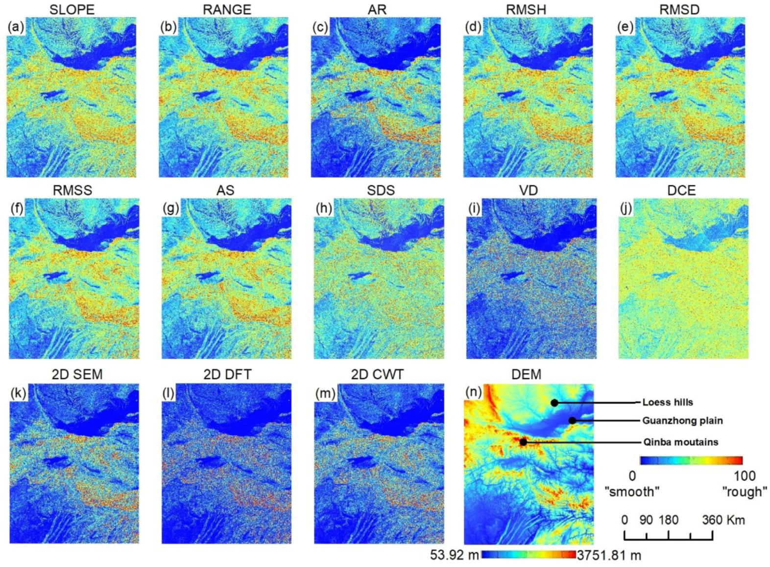
The calculation results of the various roughness algorithms in the study area showed the following (Figure 3): (1) Compared to the elevation surface, the calculated results of the various roughness algorithms represented high-frequency information and, to a certain extent, they could identify the different terrain types (such as plain, hill, and mountain) in the study area. Meanwhile, the calculated results showed good agreement with the spatial variation of the topographic types. For example, the roughness of the Qinba Mountains and loess hilly regions was obviously greater than that of the Hanzhong Basin and Guanzhong Plain. (2) The roughness values extracted by the five AR, VD, 2D SEM, 2D DFT, and 2D CWT algorithms were overall smaller, and the high values were mainly reflected in the area where the elevation of the Qinba Mountain region was changing drastically. However, these algorithms could still reflect the regional variation of the surface roughness even if the values of these algorithms were small.

4.1.2. Effect Size and Entropy

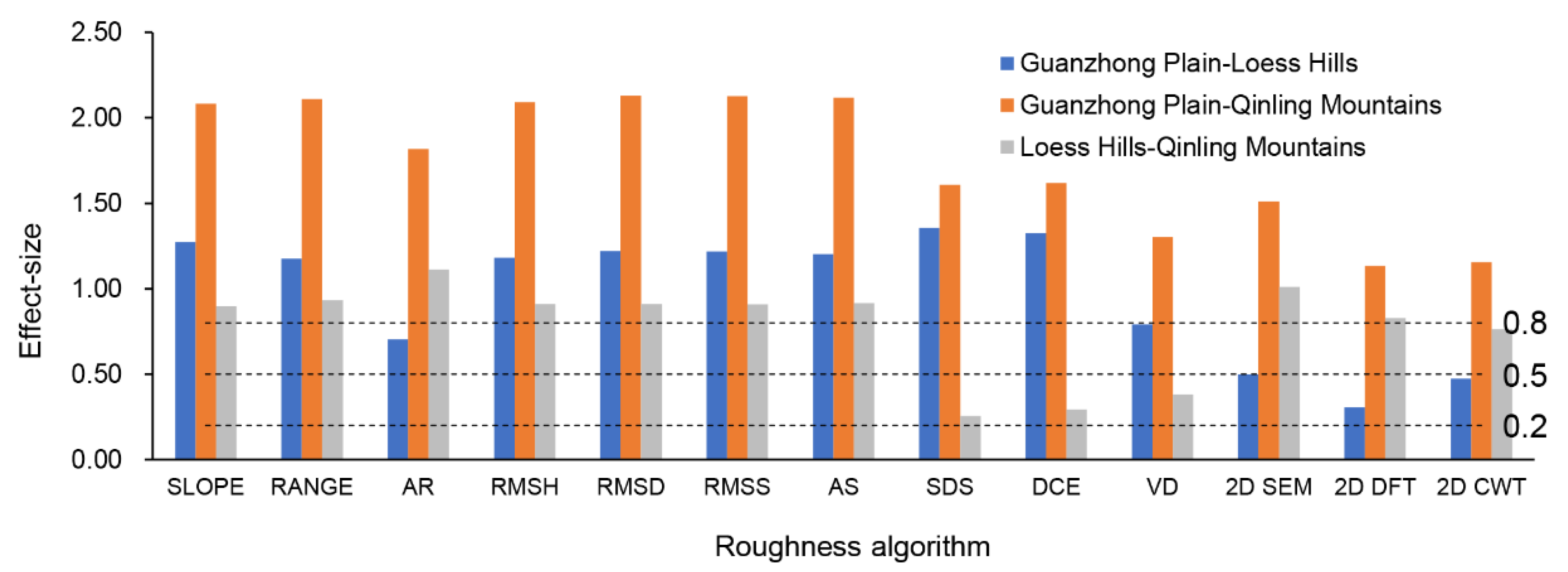
The effect size of the different roughness results in the different regions (Table 2) clearly showed that each method was able to highlight differences between the plain area and mountain area (the effect size was between 1.1 and 2.2), and there was almost no difference between the Qinling Mountains and the Bashan Mountains (with an effect size in the range of 0.01–0.28). We simplified the sample area into three groups: plain–hill, plain–mountain, and hill–mountain (Figure 4), which reflected the effect of the different roughness algorithms on terrain differences in an effective way. The results showed that SLOPE, RANGE, RMSH, RMSD, RMSS, and AS had a similar ability for terrain partition, that their effect sizes were similar (no more than 0.1 difference), and that the differences among the three sample areas were obvious (all of which were larger than 0.8). Among the rest of the algorithms, AR, VD, 2D SEM, and the frequency spectral analysis method did not show significant differences between the plain and hilly areas (with an effect value between 0.5 and 0.8). In addition, the results of the SDS, VD, and DCE algorithms showed little difference between hilly and mountainous areas (with an effect value between 0.2 and 0.5).
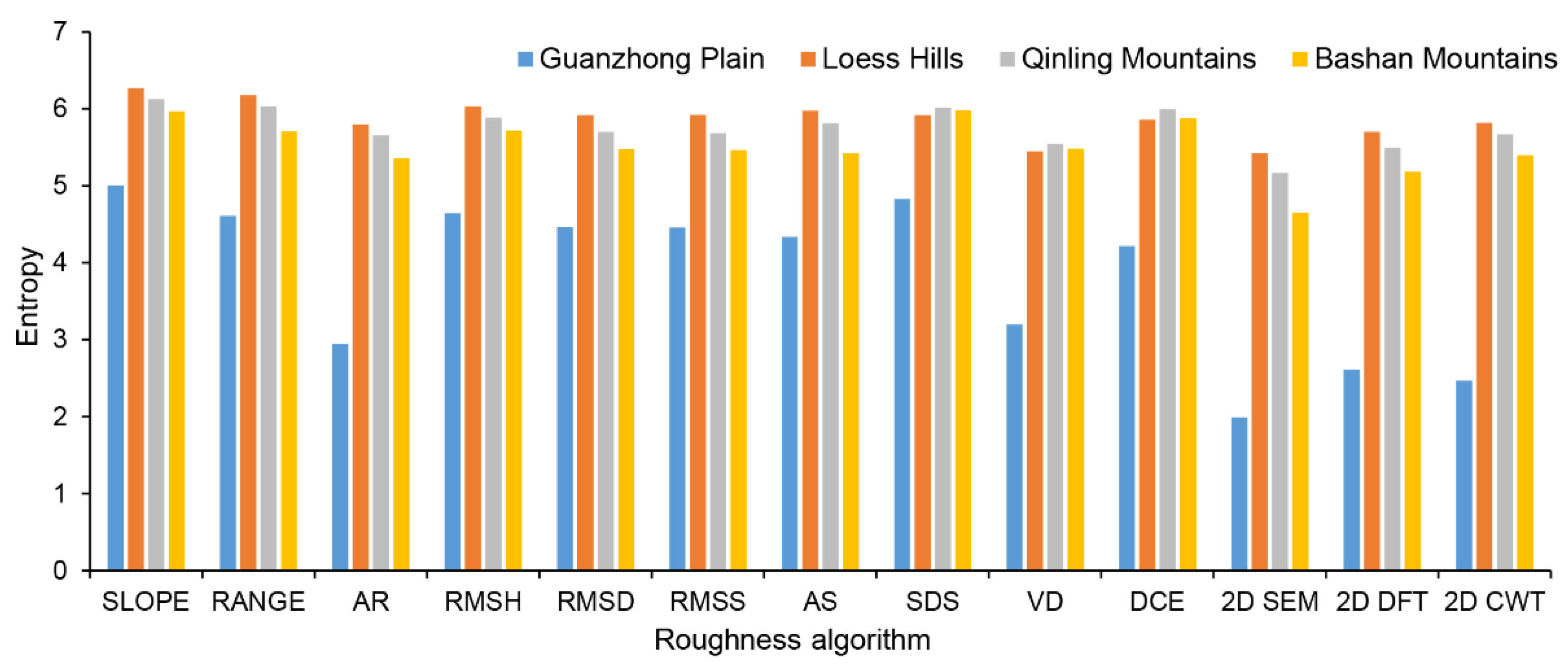
From Figure 5, it can be concluded that for different topographical areas using the same algorithm, the entropy information of areas with more complex topography (such as mountains and hills) was clearly higher than that of areas with flat terrain (such as plains), which shows that the results of these algorithms were in accordance with the distribution of the topographic structure. Among them, the information entropy of the five roughness algorithms—AR, VD, 2D SEM, 2D DFT, and 2D CWT—was slightly higher than that of other algorithms in hilly and plain areas, which means that the five roughness algorithms were more sensitive to areas with large terrain differences and they had a weak ability to represent the details of roughness in areas with less terrain relief. The difference in the information entropy of SDS, VD, and DCE was lower than that of the other algorithms, which was consistent with the results obtained for the effect size. The information entropy of different algorithms in the same area showed that SLOPE had the highest information entropy, followed by SDS, DCE, RANGE, RMSH, RMSD, RMSS, and AS, all of which had a similar order of magnitude of information entropy. Among them, the information entropy of RMSH was the highest. The entropy of the two algorithms that used spectral analysis methods was almost the same order of magnitude, and 2D CWT was better. The remaining three roughness algorithms had a lower order of magnitude of information entropy, which indicated that the roughness extraction results from the remaining three algorithms had lower integrity and complexity.
Based on this, the results of the effect size and information entropy showed that SLOPE, RANGE, RMSH, RMSD, RMSS, and AS all had a moderate ability to accurately represent and distinguish terrain types. However, AR, 2D SEM, 2D DFT, and 2D CWT were not good enough to identify regions with less topographic relief, and SDS, DCE, and VD lacked the ability to distinguish complex terrain areas.

4.1.3. Correlation between Algorithms

As mentioned before, surface roughness algorithms can be divided into three categories: Those based on elevation (or its variation), those based on the slope normal vector, and those that use spectral analysis. By calculating the correlation between the various algorithms (Table 3), it was observed that: (1) The correlation coefficient between seven algorithms—RANGE, AR, RMSH, RMSD, RMSS, AS and 2D SEM, and SLOPE—was higher than 0.8, and the correlation between the root mean square of the elevation and the SLOPE was the highest. Based on these results, we assigned these eight algorithms to a group. (2) The VD and DCE algorithms had correlation coefficients greater than 0.5 with SDS. Therefore, these three algorithms could be assigned to a group. Although two of the algorithms were based on the normal slope vector, they were independent of each other, and their correlation was not high. (3) The correlation coefficients of the two algorithms based on spectral analysis methods were greater than 0.9, so these two algorithms were assigned to one group.
In terms of the mechanisms of the algorithms, the basic meaning of the first group of algorithms was similar to that of the slope, but the specific forms were different. Although some algorithms were based on the elevation difference, the height difference per unit area within a certain distance was similar to the slope algorithm that used a fixed calculation window. In the second group of algorithms, SDS was equivalent to the third derivative of the height, which overemphasized high-frequency information, so it was not comparable to the other algorithms. VD and DCE shared a certain similarity in principle, with both describing the complexity of terrain using the spatial variability of normal vectors of surface elements. However, due to their different mathematical calculation methods, the correlation between the two algorithms was low and more independent than the results of the other algorithms. The third group used the distribution characteristics of the range information in the terrain to represent the roughness over a certain frequency range, so these algorithms were highly correlated. Additionally, because of the particularity of the spectral analysis methods compared to other algorithms, the third group of algorithms had no obvious correlation with other algorithms.
Therefore, we combined the results of the effect size and information entropy in the previous section to extract the best performance methods from each group of roughness algorithms, and then classified them into four categories: SLOPE (slope), RMSH (relief), DCE (based on the slope normal vector), and 2D CWT (based on frequency analysis).

4.2. Characteristics of the Statistical Distributions

4.2.1. Statistical Distribution

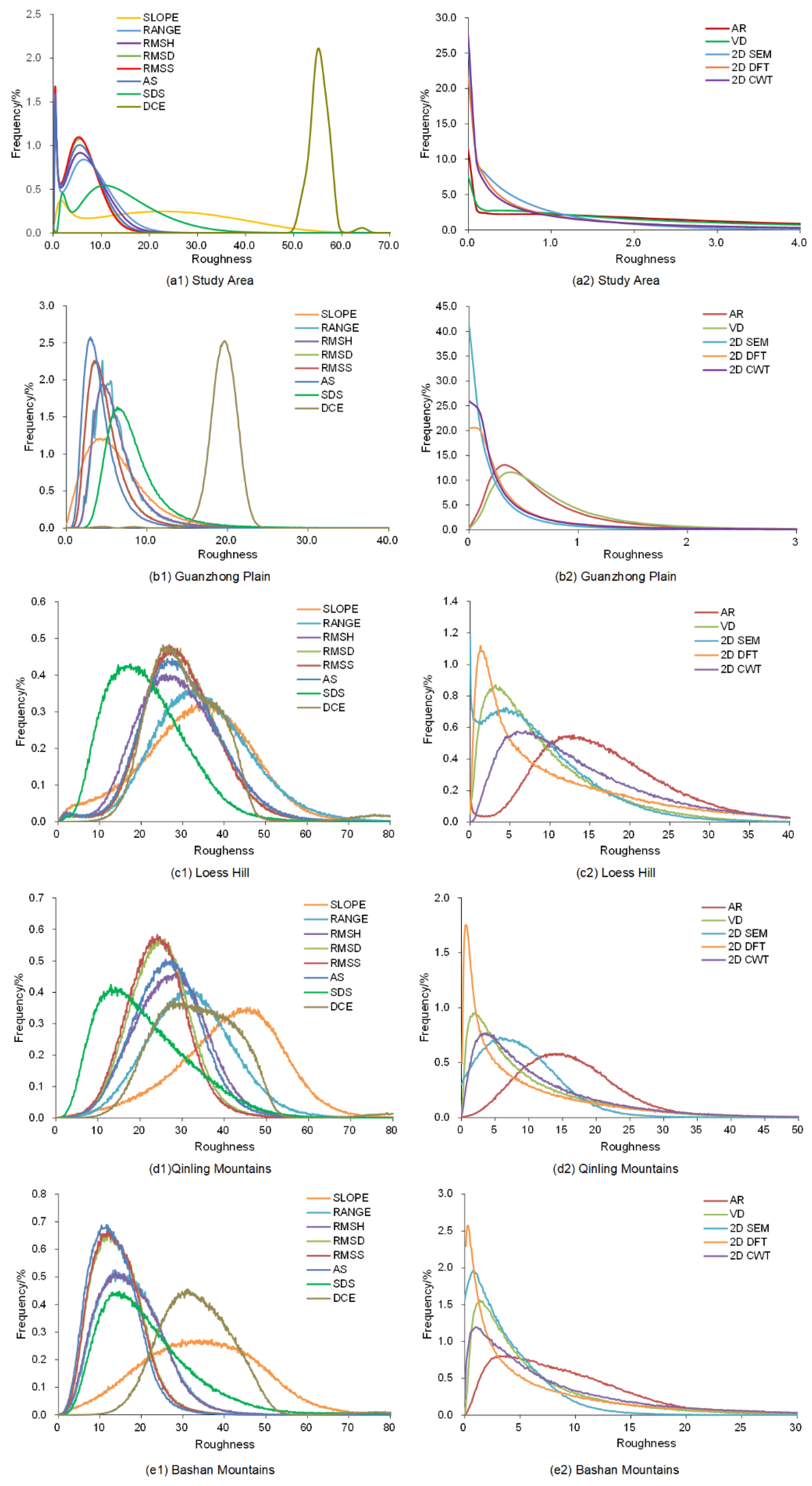
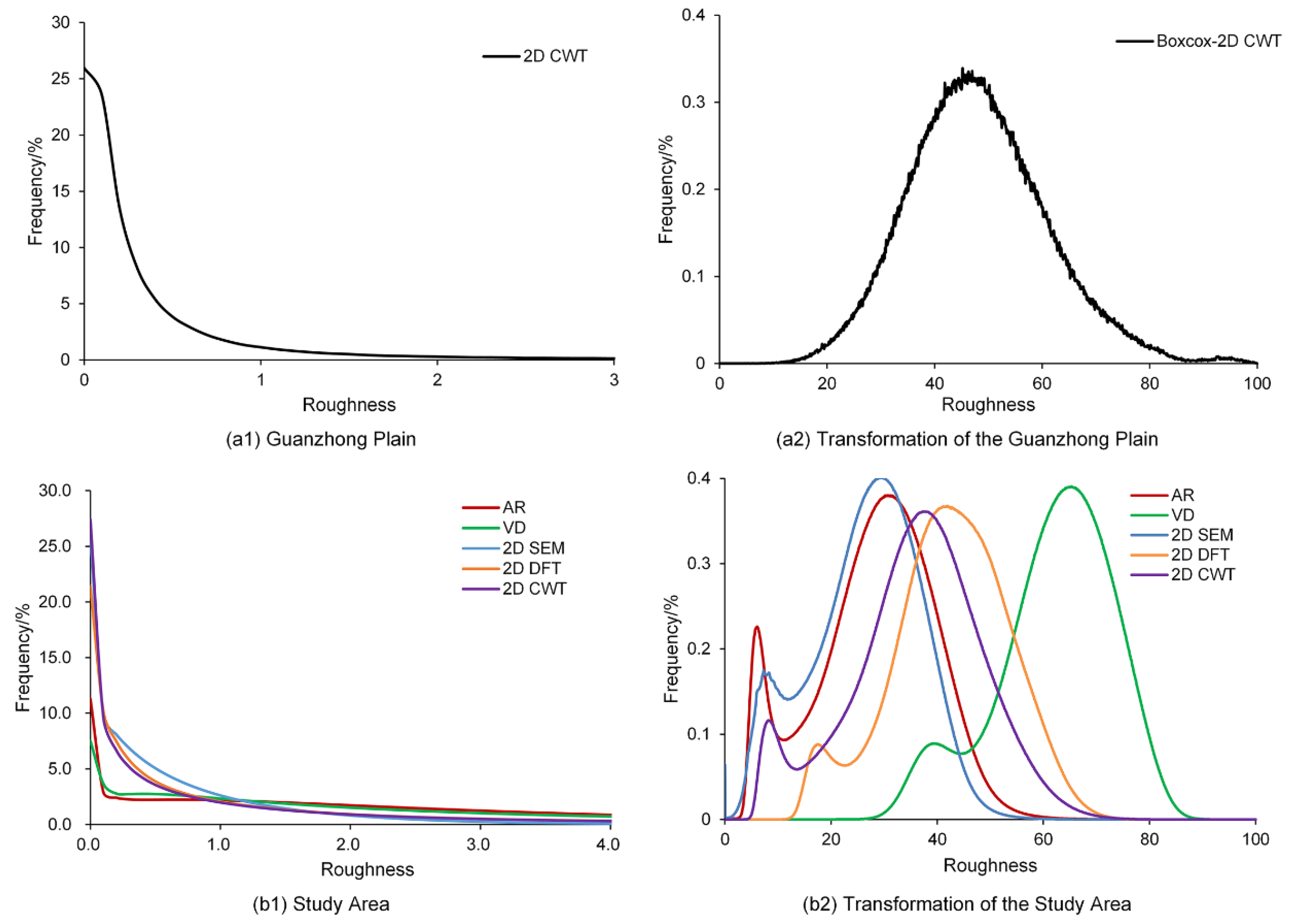
The frequency curve of the distribution of the roughness resulting from different algorithms (Figure 6) showed the following: (1) The SLOPE, RANGE, RMSH, RMSD, RMSS, AS, and SDS algorithms all had a bimodal distribution, which indicated that two types of terrain could be identified based on the above algorithms, but that the actual topographic structure should have been larger than two. In terms of the shape of the frequency curve, the differences between RANGE, RMSH, RMSD, RMSS, and AS were not clear. (2) DCE tended to have a normal distribution and was relatively independent. (3) The curve distributions of the AR, VD, 2D SEM, 2D DFT, and 2D CWT algorithms all decreased monotonically, indicating that the values of the roughness extraction of these five algorithms were small and that the distribution of the roughness values was concentrated in small regions.
For different small sample areas: (1) In bimodally distributed algorithms applied to the entire study area, the SLOPE algorithm was most similar to the normal distribution. Nevertheless, the differences between several algorithms were not obvious in terms of the frequency curve. All had a single peak distribution, which indicated a single type of topography in the sample area. (2) DCE tended to be normally distributed in the plains. In the sample areas where the topography was more complicated (hilly, mountainous), the degree of deviation was obviously increased. The change in the frequency curve was clear, but it still had a single peak. (3) In the plains, the frequency curves of AR and VD had a single peak, whereas the curve distributions of the 2D SEM, 2D DFT, and 2D CWT algorithms all monotonically decreased. In hilly and mountainous regions, although the values of the five algorithms were still concentrated in small regions, the frequency curves had a single peak distribution.

4.2.2. Transformation

In general, deviations in non-normal distribution patterns affect the accuracy of statistical results in many ways, such as during correlation analysis, regression analysis, and variance analysis. Therefore, transformation is used to avoid this effect to increase the accuracy of the results [25]. From the point of view of this study, the purpose was to quantitatively study the number of topographic types in the study region using the number of frequency peaks in histograms, which were the result of roughness calculations. Therefore, it was necessary to transform the results of the frequency histogram to a monotone descent using a transformation method. Using Guanzhong Plain as an example, the results obtained using the Box–Cox transformation were good and approximated a normal distribution. Therefore, we used this method to perform transformation in the whole region for the roughness results of five algorithms: AR, VD, 2D DFT, and 2D CWT. The results showed that the five algorithms were bimodally distributed after the transformation (Figure 7), which showed that the five algorithms could identify at least two different geomorphological types.

4.3. Terrain Partition Based on Roughness

4.3.1. Ability to Distinguish Types of Terrain

Based on the previous analysis of the spatial patterns, statistical distributions, and correlations, we removed the algorithms with high slope correlations from the 13 algorithms. We chose four algorithms to partition the terrain types: SLOPE, RMSH, DCE, and 2D CWT.
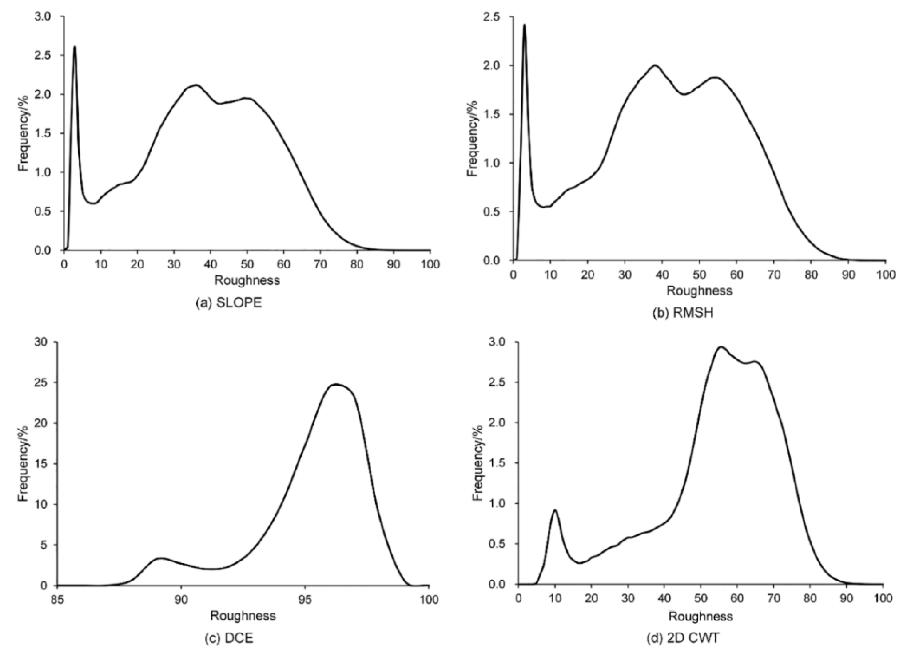
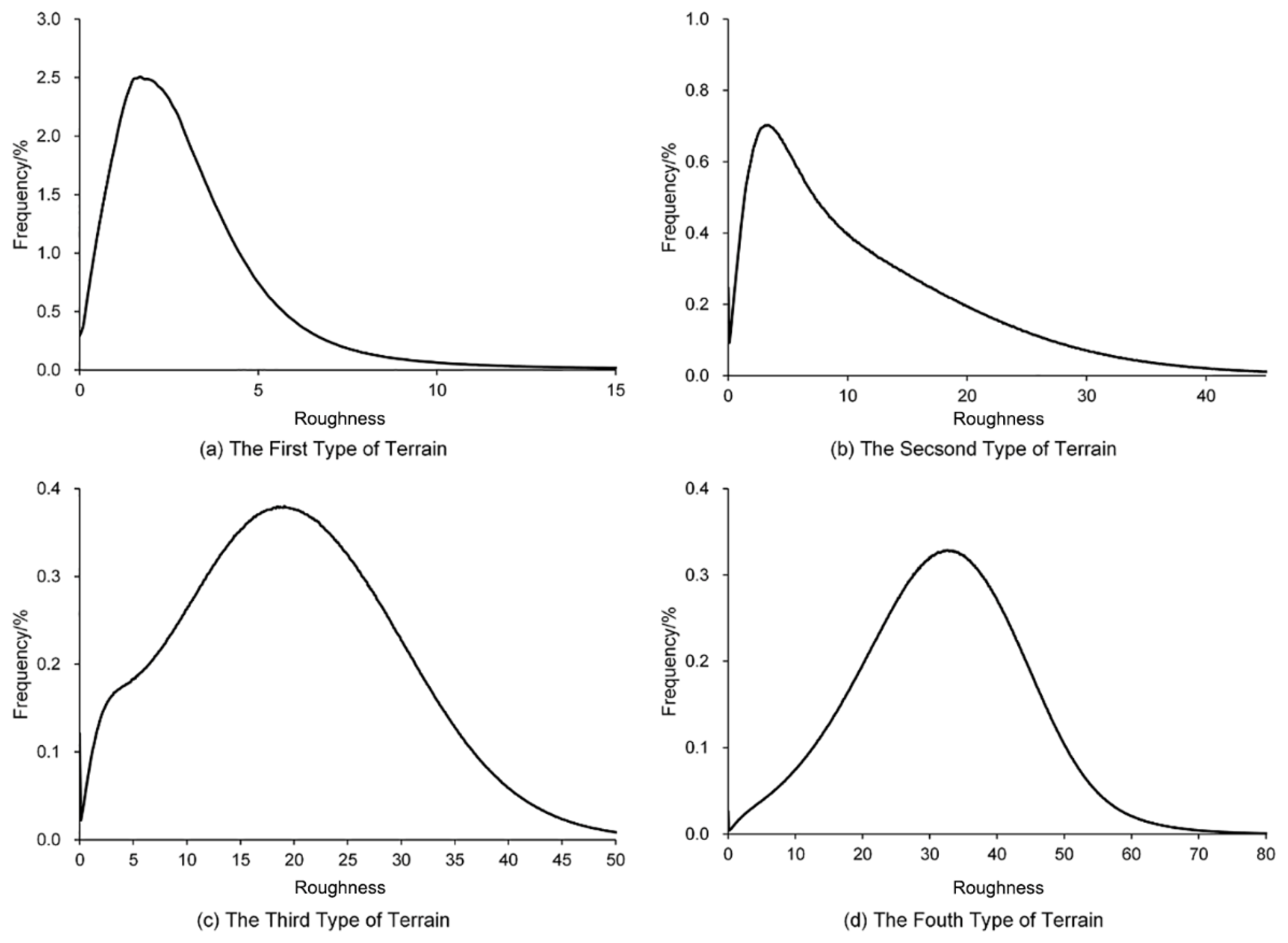
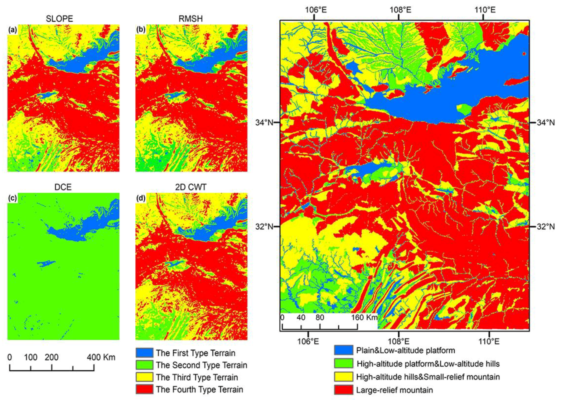
In general, the frequency curve of the single terrain had a normal distribution once it reached a mature stage [26]. Therefore, the mean filtering method was used to remove the small relief from the roughness results, and the different terrain types in the study area were classified macroscopically. After several attempts, we found that the result of a mean filter window of 41 × 41 was ideal for the SLOPE, RMSH, and DCE algorithms, whereas 2D CWT required a 71 × 71 window due to the transformation. Based on Figure 8, we used a set of conditional functions (Equation 7) to subtract the threshold value from the valley value of the frequency rate curve and partitioned the terrain type of the original roughness result. The results showed that all three methods—SLOPE, RMSH, and 2D CWT—had four peaks, which indicated that these three algorithms could recognize four types of terrain. The results of these three methods were not significantly different from each other. The 2D CWT results had a slightly more local mountainous area than the first two, which indicated that 2D CWT emphasized the high-frequency components of the earth’s surface. Using the slope as an example, the frequency curves of the four types of terrain were found to have a single peak distribution (Figure 9), which showed that the four types of terrain were relatively separate. However, the residual DCE algorithm had a poor ability to identify terrain and could only classify two macroscopic types:
RasterN = con(a ≤ rasterF or b ≤ rasterF < c or rasterF ≥ d, RasterX)
In Equation (7), rasterF is the filtered roughness result, RasterX represents the original roughness result, and RasterN represents the types of partition.
To evaluate the effect of the partition, we referred to the 1:1 million-scale geomorphologic map of China (data from the Resource and Environmental Science Data Center of the Chinese Academy of Sciences, http://www.resdc.cn). We used the same color partition to match the landmarks as much as possible to better compare the roughness results. Figure 10 shows that among the four geomorphological types partitioned by SLOPE, RMSH, and 2D CWT, the results of the partition in the plain area of the first terrain type and mountainous area of the fourth terrain type were the most ideal. High-elevation platform and low-elevation hills dominated the second type of terrain. The third type of terrain included high-altitude hills and small-relief low mountains. Although the partitioning of the second and third type of terrain was slightly weaker than that of the first and fourth types, the geomorphological type was not absolutely unique, and the partition could also express the macroscopic spatial variation of the topographic type.
To evaluate the partition ability of terrain features more accurately, we used statistics from a condition function to compare the degree of agreement between the whole study area and the four types within the original geomorphologic map (Table 4). The results showed that the discriminative ability of the SLOPE algorithm was similar to that of the RMSH algorithm. However, the results of these two algorithms for the second type of terrain were not ideal (the matching degree was only approximately 0.4). Based on the result of the 2D CWT algorithm, there were more expressive components for the third and fourth types of terrain, hills, and mountains, respectively, which indicated that the 2D CWT algorithm emphasized the high-frequency components of the surface, but its overall effect was slightly weaker than that of the first two algorithms, which was consistent with the previous results.

4.3.2. Application of Algorithms

The results of the spatial structure, statistical distribution, and terrain partition from different algorithms showed that the SLOPE and several algorithms with high correlations could better describe terrain features. As one of the roughness algorithms, SLOPE is simple to implement, and its application is mature. The result of the SLOPE algorithm showed that its information entropy was the highest, and it had significant differences for the plain–mountain and hilly areas, which indicated that SLOPE could directly and effectively represent the steepness of surface units and the spatial variability of terrain. The SLOPE algorithm was useful for partitioning terrain features. RANGE and RMSH were better among several algorithms with high correlations with SLOPE. Theoretically, the former algorithm represented the elevation range within a given range and was suitable for macroscopic analysis of the terrain relief. The latter focused on the degree of terrain dispersion (the difference between the elevation value and mean value of each pixel within the scope of the statistic), such that compared with the former, RMSH was able to represent the spatial variability of local terrain more effectively. AR and 2D SEM could also express the concave and convex changes of terrain effectively. The information entropy and effect size results showed that these two algorithms were only weakly able to express roughness details in flat terrain and could not clearly distinguish plains and hilly areas. As far as the overall effect was concerned, AR and 2D SEM were not as good as SLOPE and several other algorithms with high slope correlation. Both the DCE and VD algorithms quantify roughness using the spatial variability of the normal vector of the slope surface. These two algorithms could effectively express the irregularity of the surface according to the degree of dispersion or aggregation of the normal vectors. These two algorithms had high sensitivity to areas with large terrain differences in the aspects of the effect size and information entropy, which indicated that the two algorithms were more suitable for representing surface roughness at a fine scale. However, these algorithms had little ability to macroscopically distinguish types of terrain, as they could only distinguish two terrain types. The 2D DFT and 2D CWT algorithms can be used to distinguish the surface roughness of a particular area by analyzing the spectral characteristics in the frequency domain. Their advantage lies in the fact that they can quantify different terrain patterns according to their spatial frequency distribution characteristics, and they have the ability to distinguish terrains. Meanwhile, their defect lies in the fact that the frequency spectrum method cannot be directly transformed into a roughness index. Thus, they did not provide a clear intuitive meaning of roughness.

5. Discussion and Conclusions

5.1. Discussion

(1) Hoffman (1990) has proposed that the characteristics of roughness algorithms should have the following traits: (i) They should be able to effectively distinguish the relief, frequency, and correlation of the surface; (ii) they should be able to represent the intrinsic properties of the earth’s surface, rather than properties that arise after processing (rotation or translation); (iii) they should be able to analyze at the pixel level rather than over the entire workspace; and (iv) they should have intuitive physical meaning.
Based on these criteria, this study classified 13 roughness algorithms into four major types of algorithms based on slope, relief, normal slope vectors, and frequency analysis.
After performing correlation analysis, we found that the correlation coefficients between seven algorithms—RANGE, AR, RMSH, RMSD, RMSS, AS, and 2D SEM—had a high correlation with SLOPE. RANGE and RMSH are frequently used as common indexes to evaluate relief. The former expresses the height difference in a specific range. RMSH calculates the difference between the height and mean value of each pixel in a moving window, so the expression of spatial variation in local scopes is better in RMSH than in the other two algorithms. Therefore, RMSH was chosen as the optimal algorithm for the degree of relief. In essence, RMSS and AS are slope’s variants. Both algorithms express roughness as the degree of local variation (the ratio of the height difference to the horizontal distance) of the surface elevation. AR measures roughness as the ratio of the surface area to the projected area, but the low slope value is compressed because of the triangle function of slope, which leads to a weak ability to distinguish low-relief areas. Thus, the different topographic features could not be well represented. The 2D SEM algorithm also expresses the spatial difference of the surface elevation value. This algorithm calculates the square of the local surface height difference and highlights the obvious aspect of the surface elevation change. Therefore, the effect of 2D SEM was similar to that of AR because the difference was not significant in areas with low relief. Overall, all of the algorithms with high correlations with SLOPE have a substantial meaning similar to slope.
However, the slope algorithm is mature and easy to implement, and various analyses show that it has a significant ability to distinguish types of terrain. Moreover, the slope algorithm is not affected by the calculation window size, so SLOPE and RMSH were selected as the optimal algorithms of the group.
In the second group of algorithms, SDS is equivalent to the third derivative of the elevation. SDS overemphasizes high-frequency information, and although it is able to express the complexity of slope changes in a local area, it cannot be compared to other algorithms. Both VD and DCE are roughness algorithms based on slope normal vectors: They have the same basis, but use different methods to calculate the aggregation degree of the normal vectors. Therefore, there are some differences between them. Thus, the results of DCE are better than those of VD from various analytical perspectives.
The algorithms that use the spectral analysis method can express the distribution characteristics of amplitude information over a certain frequency range. However, 2D CWT transforms discrete data into the spatial–frequency domain and provides the frequency distribution of the terrain’s amplitude information at every location in space. Meanwhile, this algorithm selects the range of the wavelet scale parameter to extract the corresponding frequency range of the surface roughness features. Thus, this algorithm is more optimized than the 2D Fourier transform. Therefore, we chose the 2D CWT to evaluate the final partitioning of terrain features.
(2) Currently, with the development of advanced surveying technology, roughness algorithms have become increasingly mature, which is reflected in the improvement of data resolution. With the expansion of the scope of monitoring and the diversity of topographic data sets, it has become a new trend to combine the former roughness theory research with advanced surveying technology to quantitatively describe topographic changes and formation processes [27,28]. In recent years, an increasing amount of high-resolution terrain data have been used to determine the complexity of small-scale features (such as hillslope). In other words, with the increase of the precision of data, the microterrain and geomorphic information that cannot currently be determined from low-resolution data will be able to be evaluated. Nevertheless, roughness research at large, medium, and small scales inevitably requires the selection of a DEM with an appropriate resolution and a window with an appropriate size, which is helpful for improving the efficiency of data operations and the accuracy of the results. Therefore, the relationship between different scales of research and optimal demand is a problem that still needs to be explored.
(3) The conclusion of this study assigned the 13 roughness algorithms to four categories, then analyzed and evaluated their ability to partition terrain. It was mainly aimed at the macroscopic partition of different topographic types, such as plain, loess hills, and mountainous areas. Moreover, the analysis results were relatively accurate. Therefore, the results have certain universality for terrain differentiation with large differences within a large-scale study area, but the results still need to be verified by actual derivation in regions where the small-scale difference is not significant.
With the new DEMs that are becoming available, based on the different data sources with the input data to extract roughness (e.g., Aster GDEM, TanDEM-X DEM), the potential impact of DEM data on the results of the analysis is also a meaningful research area.
(4) The slope roughness is the variation of the angle that the normal to a slope facet makes with the gravity normal. This drives water and soil movement and land sliding. Surface texture roughness applies to a plane surface as well as to slopes, and does not specifically involve the gravity normal. It is a more detailed variation and affects resistance to flows over the surface. This research was most interested in slope roughness. However, with higher resolutions of input data, finer detail surface textures are also valuable and are being addressed in methods of spectral analysis. Finer detail surface textures are perhaps the next stage of roughness research after primary slope roughness classification.

5.2. Conclusions

On the basis of the representative roughness algorithm studied in previous research, we integrated and compared 13 roughness algorithms with slope and terrain relief as the indexes to measure roughness in this study. The results were as follows.
(1)
An ideal roughness algorithm should have the ability to distinguish surface relief (spatial patterns and statistical distributions). From the macro point of view, the 13 algorithms were able to express the spatial variability of the terrain from image surface features to some extent, but there were some differences in their spatial patterns and statistical distributions. In terms of the ability to express and distinguish the terrain, the effect of slope is relatively strong, and the SLOPE algorithm is mature and easy to calculate and distinguishes the four types of terrain in the study area. The statistical distribution characteristics of these four types of terrain had a single peak distribution according to the slope algorithm. The seven roughness algorithms that had a high slope correlation were RANGE, AR, RMSH, RMSD, RMSS, AS, and 2D SEM, and the results of RMSH were the best in terms of the spatial pattern, statistical distribution, and ability to distinguish terrain types. The advantage of the algorithms based on spectral analysis was that they could quantify different terrain patterns according to different frequency bands and had an equivalent ability to partition terrain as the slope-based methods after canonical transformation. SDS, DCE, and VD have the general ability to distinguish terrain and can only classify two types of terrain.
(2)
In terms of applicability, the SLOPE algorithm could directly reflect the degree of steepness and irregularity of the surface unit. Among several algorithms having high correlation with SLOPE, RANGE could express the undulation of terrain over a relatively wide range of heights, and RMSH focused on expressing the degree of discreteness of the terrain. These algorithms could distinguish terrain well. SDS, DCE, and VD were not suitable for distinguishing terrain features, as the former algorithm is used to represent the complexity of slope variation in local areas, whereas the latter two are more suited for the extraction of terrain features at a fine scale. Two algorithms based on spectral analysis could be used to extract the required frequency components by adjusting the range of characteristic frequencies. Although the obtained spectral parameters could not be directly transformed into roughness indexes, and there was no clear and intuitive roughness meaning, the advantage was that they can quantify different topographic patterns and features according to the spatial characteristics of the frequency distribution.

Author Contributions

Q.Y. is responsible for the original idea; J.W. performed the experiments and wrote the paper; Y.L. contributed to analysis of the data; Q.Y. contributed to revising the paper.

Funding

This research was funded by the National Natural Science Foundation of China: study on theoretical distribution model of slope (grant number 41371274).

Acknowledgments

The author is grateful to the editor and anonymous reviewers for spending their valuable time on constructive comments and suggestions that improved the quality of the manuscript considerably.

Conflicts of Interest

The authors declare no conflicts of interest.

References

  1. Hani, A.F.M.; Sathyamoorthy, D.; Asirvadam, V.S. A method for computation of surface roughness of digital elevation model terrains via multiscale analysis. Comput. Geosci. 2011, 37, 177–192. [Google Scholar] [CrossRef]
  2. Shepard, M.K.; Campbell, B.A.; Bulmer, M.H.; Farr, T.G.; Gaddis, L.R.; Plaut, J.J. The roughness of natural terrain: A planetary and remote sensing perspective. J. Geophys. Res. Planets 2001, 106, 32777–32795. [Google Scholar] [CrossRef] [Green Version]
  3. Grohmann, C.H.; Smith, M.J.; Riccomini, C. Multiscale analysis of topographic surface roughness in the midland valley, scotland. IEEE Trans. Geosci. Remote Sens. 2011, 49, 1200–1213. [Google Scholar] [CrossRef]
  4. Lv, Y.L.; Li, G.Y. Surface roughness and soil wind erosion. Adv. Soil Sci. 1992, 38–42. [Google Scholar]
  5. Lawless, M.; Robert, A. Scales of boundary resistance in coarse-grained channels: Turbulent velocity profiles and implications. Geomorphology 2001, 39, 221–238. [Google Scholar] [CrossRef]
  6. Lacey, R.W.J.; Roy, A.G. The spatial characterization of turbulence around large roughness elements in a gravel-bed river. Geomorphology 2008, 102, 542–553. [Google Scholar] [CrossRef]
  7. Jester, W.; Klik, A. Soil surface roughness measurement—Methods, applicability, and surface representation. Catena 2005, 64, 174–192. [Google Scholar] [CrossRef]
  8. Smith, M.W. Roughness in the earth sciences. Earth-Sci. Rev. 2014, 136, 202–225. [Google Scholar] [CrossRef]
  9. Hobson, R.D. Surface Roughness in Topography: Quantitative Approach. In Spatial Analysis in Geomorphology; Methuen & Co.: London, UK, 1972; pp. 221–245. [Google Scholar]
  10. Hoffman, R.; Krotkov, E. Terrain roughness measurement from elevation maps. Int. Soc. Optics Photon. 1990, 4, 104–114. [Google Scholar] [CrossRef]
  11. Mckean, J.; Roering, J. Objective landslide detection and surface morphology mapping using high-resolution airborne laser altimetry. Geomorphology 2004, 57, 331–351. [Google Scholar] [CrossRef]
  12. Glenn, N.F.; Streutker, D.R.; Chadwick, D.J.; Thackray, G.D.; Dorsch, S.J. Analysis of lidar-derived topographic information for characterizing and differentiating landslide morphology and activity. Geomorphology 2006, 73, 131–148. [Google Scholar] [CrossRef]
  13. Booth, A.M.; Roering, J.J.; Perron, J.T. Automated landslide mapping using spectral analysis and high-resolution topographic data: Puget sound lowlands, washington, and portland hills, oregon. Geomorphology 2009, 109, 132–147. [Google Scholar] [CrossRef]
  14. Pommerol, A.; Chakraborty, S.; Thomas, N. Comparative study of the surface roughness of the moon, mars and mercury. Planet. Space Sci. 2012, 73, 287–293. [Google Scholar] [CrossRef]
  15. Berti, M.; Corsini, A.; Daehne, A. Comparative analysis of surface roughness algorithms for the identification of active landslides. Geomorphology 2013, 182, 1–18. [Google Scholar] [CrossRef]
  16. Lane, S.N. Roughness—Time for a re-evaluation? Earth Surf. Process. Landf. 2010, 30, 251–253. [Google Scholar] [CrossRef]
  17. Moore, I.D.; Grayson, R.B.; Ladson, A.R. Digital terrain modelling: A review of hydrological, geomorphological, and biological applications. Hydrol. Process. 2010, 5, 3–30. [Google Scholar] [CrossRef]
  18. Jiang, H.S.; Yang, Q.K. Algorithm comparison of relief amplitude based on dynamic effect mode. Bull. Soil Water Conserv. 2014, 34, 162–166. [Google Scholar] [CrossRef]
  19. Evans, I.S. An integrated system of terrain analysis and slope mapping. Zeitschrift für Geomorphologie 1980, 36, 274–295. [Google Scholar]
  20. Frankel, K.L.; Dolan, J.F. Characterizing arid region alluvial fan surface roughness with airborne laser swath mapping digital topographic data. J. Geophys. Res. Earth Surf. 2007, 112, 325–327. [Google Scholar] [CrossRef]
  21. Kreslavsky, M.A.; III, J.W.H. Kilometer-scale slopes on mars and their correlation with geologic units: Initial results from mars orbiter laser altimeter (mola) data. J. Geophys. Res. Planets 1999, 104, 21911–21924. [Google Scholar] [CrossRef]
  22. Cohen, J. Statistical Power Analysis for the Behavioral Sciences; L. Lawrence Earlbaum Associates: Hillsdale, NJ, USA, 1988; Volume 2. [Google Scholar]
  23. Shannon, C.E. A mathematical theory of communication: The bell system technical journal. J. Frankl. Inst. 1938, 196, 519–520. [Google Scholar]
  24. Box, G.E.P.; Cox, D.R. An analysis of transformations. J. R. Stat. Soc. 1964, 26, 211–252. [Google Scholar] [CrossRef]
  25. Csillik, O.; Evans, I.S.; Drăguţ, L. Transformation (normalization) of slope gradient and surface curvatures, automated for statistical analyses from dems. Geomorphology 2015, 232, 65–77. [Google Scholar] [CrossRef]
  26. Wolinsky, M.A.; Pratson, L.F. Constraints on landscape evolution from slope histograms. Geology 2005, 33, 477–480. [Google Scholar] [CrossRef]
  27. Bretar, F.; Arab-Sedze, M.; Champion, J.; Pierrot-Deseilligny, M.; Heggy, E.; Jacquemoud, S. An advanced photogrammetric method to measure surface roughness: Application to volcanic terrains in the piton de la fournaise, reunion island. Remote. Sens. Environ. 2013, 135, 1–11. [Google Scholar] [CrossRef]
  28. Jiang, Y.C.; Fang, H.L.; Wei, S.S. Review of land surface roughness parameterization studyreview of land surface roughness parameterization study. Adv. Earth Sci. 2012, 27, 292–303. [Google Scholar]
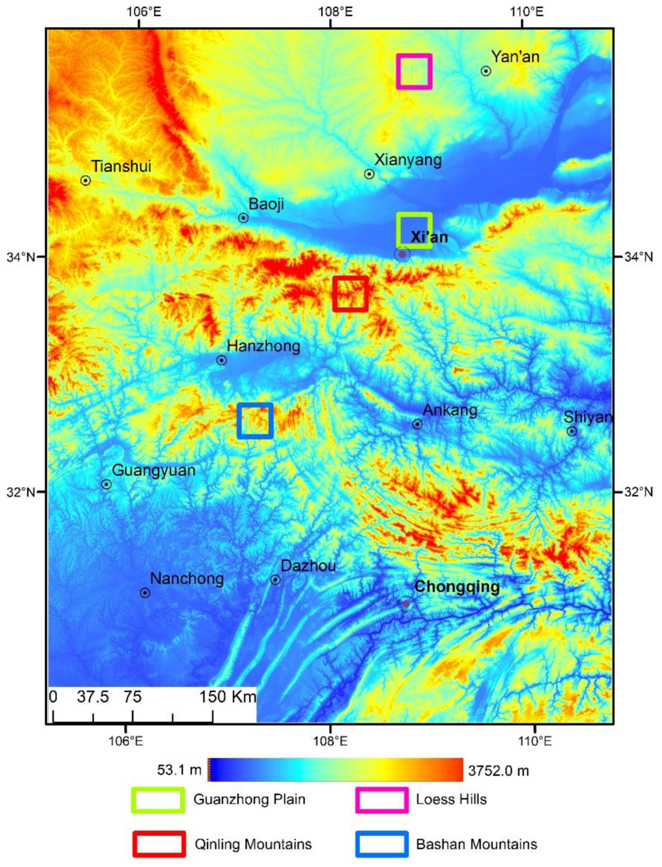
Figure 1. Map of the study area (digital elevation model derived from 1″ Shuttle Radar Topographic Mission (SRTM) data).
Remotesensing 10 01985 g001
Figure 2. Schematic block diagrams showing how the surface roughness of the terrain can be reflected by the unit direction vector of each pixel in a digital elevation model (DEM). If the ground surface is smooth, the unit direction vectors are aggregative. If the ground surface is rough, the unit direction vectors are dispersed.
Remotesensing 10 01985 g002
Figure 3. Extraction results of the different roughness algorithms: (a) SLOPE; (b) RANGE; (c) AR; (d) RMSH; (e) RMSD; (f) RMSS; (g) AS; (h) SDS; (i) VD; (j) DCE; (k) 2D SEM; (l) 2D DFT; (m) 2D CWT; (n) original SRTM.
Remotesensing 10 01985 g003
Figure 4. Comparison of the effect sizes between different roughness algorithms in different regions.
Remotesensing 10 01985 g004
Figure 5. Information entropy of different roughness algorithms.
Remotesensing 10 01985 g005
Figure 6. (a) Frequency curves of different roughness algorithms of whole study area; (b) Frequency curves of different roughness algorithms of Guanzhong plain sample area; (c) Frequency curves of different roughness algorithms of loess hill sample area; (d) Frequency curves of different roughness algorithms of Qinling mountains sample area; (e) Frequency curves of different roughness algorithms of Bashan mountains sample area.
Remotesensing 10 01985 g006
Figure 7. (a) The frequency curves after canonical transformation of the 2D CWT of Guanzhong plain; (b) The frequency curves after canonical transformation of the roughness algorithm of whole study area.
Remotesensing 10 01985 g007
Figure 8. (a)Frequency distribution curves of SLOPE after mean filtering; (b) Frequency distribution curves of RMSH after mean filtering; (c) Frequency distribution curves of DCE after mean filtering; (d) Frequency distribution curves of 2D CWT after mean filtering
Remotesensing 10 01985 g008
Figure 9. (a) Frequency curves of the SLOPE partition of plain; (b) Frequency curves of the SLOPE partition of high-altitude platforms and low-altitude hills; (c) Frequency curves of the SLOPE partition of high-altitude hills and low-relief mountains; (d) Frequency curves of the SLOPE partition of high-relief mountains.
Remotesensing 10 01985 g009
Figure 10. Results of the terrain partition based on geomorphological types and different roughness algorithms in the study areas. (a) Results of the terrain partition of SLOPE; (b) Results of the terrain partition of RMSH; (c) Results of the terrain partition of DCE; (d) Results of the terrain partition of 2D CWT.
Remotesensing 10 01985 g010
Table 1. Algorithms of roughness.
Sequence NumberAlgorithms (ALG)FormulaDimension
1Slope (SLOPE) θ = a r c tan p 2 + q 2
p , q = ( H x , H y )
Degree
2Local Elevation Range (RANGE) R a n g e = H m a x H m i n m
3Area Ratio (AR) A R = i = 1 N 2 1 cos S i None
4Root Mean Squared Height (RMSH) R M S H = 1 N 2 1 i = 1 N 2 ( H i H ¯ ) 2 m
5RMS Deviation (RMSD) R M S D = 1 4 ( N 1 ) b = 1 4 ( N 1 ) ( H c H b ) 2 m
6RMS Slope (RMSS) R M S S = 1 4 ( N 1 ) b = 1 4 ( N 1 ) ( H c H b Δ x b ) 2 Degree
7Absolute Slope (AS) A S = 1 4 ( N 1 ) b = 1 4 ( N 1 ) | ( H c H b ) | c ( N 1 ) 2 Degree
8Standard Deviation of Slope (SDS) S D S = 1 N 2 i = 1 N 2 ( S i S ¯ ) 2 Degree
9Vector Dispersion (VD) V D = ( N 2 R ) ( N 2 1 ) None
10Direction Cosine Eigenvalue (DCE) D C E = [ ln ( S 1 / S 2 ) ] 1 None
112D Semivariogram (2D SEM) γ = 1 2 n i = 1 n [ z ( x i , y i ) z ( x i + h , y i + h ) ] 2 m2
12Discrete Fourier Transform (2D DFT) D F T = f f 1 f 2 V D F T ( f ) m2
13Continuous Wavelet Transform (2D CWT) C W T = f f 1 f 2 V C W T ( f ) m2
Note: In the roughness algorithms, p and q denote the rate of change of height in the x and y directions, respectively. H m a x is the maximum height value of a pixel in the moving window. H m i n is the minimum height value of a pixel in the moving window. N refers to the width of the moving window (the number of pixels). H i is the height value of the pixel in the moving window. H ¯ is the average height value of pixels in the moving window. H b is the height value of pixels in the moving window edge, and Δ x b is the distance from the center pixel to the edge pixel. S i is the slope value of the ith pixel in the moving window (in radians). S ¯ is the mean value of the average slope of pixels in the moving window. R refers to vector strength, which is the square root of the sum of the squared three cosine components and the square root of the three cosine components. S 1 and S 2 are eigenvalues obtained in the 3 × 3 direction cosine matrix. X i and   Y i are the spatial coordinates of the ith pixel in a moving window, h is the lag distance, and f 1 and f 2 represent the lower limit and upper limit of the typical frequency range of terrain roughness. V D F T is the power spectrum of the 2D Fourier transform. V C W T is the power spectrum of the 2D continuous wavelet transform.
Table 2. Effect size for different roughness values in different regions.
ALGEffect Size
Guanzhong Plain–Loess HillsGuanzhong Plain–Qinling MountainsGuanzhong Plain–Bashan MountainsLoess Hills–Qinling MountainsLoess Hills–Bashan MountainsQinling Mountains–Bashan Mountains
SLOPE1.2732.0831.8370.8990.6450.245
RANGE1.1752.1091.8530.9340.6780.257
AR0.7031.8161.5421.1130.8390.274
RMSH1.1812.0921.8450.9110.6640.247
RMSD1.2202.1311.8820.9110.6610.250
RMSS1.2182.1261.8770.9090.6600.249
AS1.2032.1181.8630.9160.6610.255
SDS1.3551.6091.6370.2540.2820.028
DCE1.3251.6191.5480.2940.2230.071
VD0.7921.3021.0840.4270.2620.218
2D SEM0.4991.5091.2931.0100.7940.216
2D DFT0.3061.1340.9650.8280.6590.169
2D CWT0.4731.1551.1390.7620.6660.016
Table 3. Correlation between the extraction results of the roughness algorithm and the slope.
ALGSLOPERANGEARRMSHRMSDRMSSASSDSDCEVD2D SEM 2D DFT2D CWT
SLOPE1.0000
RANGE0.94201.0000
AR0.86550.94201.0000
RMSH0.96710.98710.94911.0000
RMSD0.94030.98040.95420.98971.0000
RMSS0.94420.97920.95400.99050.99971.0000
AS0.94470.97640.95100.99070.99580.99591.0000
SDS0.45730.47910.46300.48700.54110.53960.49531.0000
VD0.25900.32680.37570.31290.40700.40290.36810.73831.0000
DCE0.33660.35730.31120.35190.39500.39280.37570.55080.51911.0000
2D SEM0.81910.89500.94660.90340.88340.88260.88890.28640.18130.11551.0000
2D DFT0.28330.31910.34390.31790.34440.34260.32720.42740.25670.40690.24931.0000
2D CWT0.26930.30550.32850.30140.33340.33120.31480.44710.27810.45720.21640.90131.0000
Table 4. Comparison of the terrain partition results to geomorphologic maps from different roughness algorithms.
AlgStudy AreaThe First Type of TerrainThe Second Type of TerrainThe Third Type of TerrainThe Fourth Type of Terrain
SLOPE0.6820.6090.4070.5610.814
RMSH0.6800.5890.4210.5620.824
2D CWT0.6370.5020.4080.6170.863