Abstract
Multisource remote sensing data acquisition has been increased in the last years due to technological improvements and decreased acquisition cost of remotely sensed data and products. This study attempts to fuse different types of prospection data acquired from dissimilar remote sensors and explores new ways of interpreting remote sensing data obtained from archaeological sites. Combination and fusion of complementary sensory data does not only increase the detection accuracy but it also increases the overall performance in respect to recall and precision. Moving beyond the discussion and concerns related to fusion and integration of multisource prospection data, this study argues their potential (re)use based on Bayesian Neural Network (BNN) fusion models. The archaeological site of Vésztő-Mágor Tell in the eastern part of Hungary was selected as a case study, since ground penetrating radar (GPR) and ground spectral signatures have been collected in the past. GPR 20 cm depth slices results were correlated with spectroradiometric datasets based on neural network models. The results showed that the BNN models provide a global correlation coefficient of up to 73%—between the GPR and the spectroradiometric data—for all depth slices. This could eventually lead to the potential re-use of archived geo-prospection datasets with optical earth observation datasets. A discussion regarding the potential limitations and challenges of this approach is also included in the paper.
Keywords:
remote sensing archaeology; fusion; neural networks; re-use; GPR; spectral signatures; Hungary 1. Introduction
The use of remote sensing data and interpretation for archaeological mapping “is not without risks and challenges. By limiting time spent in the field, and not visiting the majority of identified sites, the approach requires the development of experience and trust in interpreting remote sensed data” [1] (emphasis added). Indeed, besides the long-recognized problems and challenges, “archaeological remote sensing has much to contribute to the future of heritage management and archaeological research” [2].
Multi-sensor data fusion intended for archaeological research is considered a promising but ambitious and challenging task [2,3]. While the application of various prospection methods has been widely adopted by archaeologists [4], the complementary use and fusion of different archaeological prospection data has been identified by the literature as an active area in the field of archaeological remote sensing where further research is required [2]. Indeed, each sensor has its own advantages and disadvantages providing different outcomes in the archaeological context. For instance, ground penetrating radar (GPR) is an active ground sensor able to penetrate ground surface and, therefore, provide 3-D information about sub-surface anomalies. In contrast, passive sensors such as optical satellite sensors or ground spectroradiometers are able to identify spectral anomalies (e.g., crop marks) of the ground surface—in different wavelengths—that are used as proxies for the detection of buried archaeological remains (see more at [5]).
Beyond archaeological applications, the fusion of data obtained from satellite remote sensing sensors has already been well documented. Since each sensor operates on a specific wavelength range and is sensitive to specific environmental conditions, the acquisition of all the required information for detecting an object is not feasible to be acquired by a single sensor. It is, therefore, not surprising that advanced analytical or numerical image fusion techniques have been developed for improved exploitation of multisource data [6]. The importance of fusion is also highlighted by [5] where image fusion provides the capability of combining two or more different images into a single image, expanding this way the information content. At the same time, the fusion process is applicable on a number of various scales (e.g., multi-scale transforms). Combination and fusion of complementary sensors not only increases detection accuracy, but also improves the performance in respect to recall and precision.
In archaeological research and practice, data fusion can enhance and reveal unknown buried features (i.e., image anomalies) [4]. Though different data fusion models and strategies that were reported in the past (see introduction part of [5]), it is shown that their application is limited to superimposition and GIS-layering of geo-datasets for visual and/or semi-automatic multilayer analysis (e.g., [7,8,9,10]). For instance, Yu et al. [11] investigated new methodologies for detecting archaeological features in Northern and Southern China based on multi-source remotely sensed data. However, the overall multi-temporal and multi-scale results were only visually cross-compared with each other. Moreover, data integration is often restricted to similar nature of data (e.g., data obtained from satellite sensors such as pan-sharpening techniques [12,13,14,15], data enhancement of geophysical prospection data [16,17,18,19], etc.).
Recent studies highlight the fact that for many archaeological sites around the world a wealth of digital, spatial, and open remotely sensed data already exists [20]. Large scale applications based on big data engines of earth observation have also been reported in the literature [21,22,23]. It is, therefore, more relevant than ever to explore new ways of fusion of multisource remotely sensed data (archived or not) moving beyond the well-established practices.
The current study is part of an ongoing research; its primary results have been presented in [5]. In that particular study, a few regression models were analyzed between GPR results and vegetation spectral indices. The regression models revealed a medium-correlation between these two different types of data for the superficial layers of an extensive archaeological landscape in Central Europe. Overall, the study concluded that fusion models between various types of remote sensing datasets can further expand the current capabilities and applications for the detection of buried archaeological remains and highlighted the need of more complex fusion models—rather than simple regression models—to further improve the fitting between the various prospection data and minimizing potential errors.
This study firstly attempts to fuse different types of prospection data acquired from dissimilar remote sensors based on a neural network architecture and secondly explores new ways of manipulating remote sensing data already obtained from an archaeological site. This exploration could lead to the re-usage of archived geo-prospection datasets.
The paper is organized as follows: at first, a short introduction of the case study area is presented, followed by a presentation of the available data and the methodology used. Then, the results are presented and discussed. The paper ends with some major conclusions as well as thoughts for future investigations.
2. Methodology and Case Study Area
2.1. Case Study Area
The case study area (Vésztő-Mágor Tell) is located in the southeastern Great Hungarian Plain (Figure 1). The Tell covers about 4.25 hectares and rises to a height of about 9 m above mean sea level. This area was intensively investigated in the previous years as part of the Körös Regional Archaeological Project [24] with various non-invasive techniques, including magnetometry, ground penetrating radar, electrical resistance tomography, hyperspectral spectroradiometry, and soil chemistry. The aim of the general project was to reconstruct the organization of the Neolithic tell-based settlements of Vésztő-Mágor and Szeghalom-Kovácshalom.
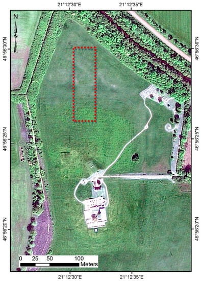
Figure 1.
Case study area—Vésztő-Mágor Tell: The red polygon indicates the area covered from the geophysical survey (GPR measurements) and ground spectroradiometric measurements (Latitude: 46°56′24.36′′; Longitude: 21°12′32.67′′, WGS84) (Figure from [5]).
During the 70s and 80s, excavations were contacted aiming to study the archaeological context of the Tell. During these studies, it was revealed that the area was initially settled by Szakálhát culture farmers during the late Middle Neolithic period, while the area was systematically occupied until the Late Neolithic period (c. 5000–4600 B.C. calibrated). On top of the Late Neolithic levels, a buried humic layer suggests the abandonment of the site until the formation of an Early Copper Age settlement and later on by a Middle Copper Age settlement. Later on, in the 11th century AD a church followed by a monastery were established on top of the Tell. The monastery operated until the end of the 14th century and the two towers of the church were standing until 1798. After various modifications, and reconstructions, the monastery was completely destroyed by the operations that were carried out during the construction of a wine cellar during the early 19th century. The site became one of the Hungarian National Parks in the 1980s. Currently, in addition to the archaeological museum located within the historic wine cellar, the 1986 excavation trench can be seen with a number of features from different periods remain in situ. More information regarding the archaeological context can be found in [25,26,27,28,29,30].
2.2. Data Soruces
Two different types of data have been used in this study: (a) ground spectral signatures collected from the GER-1500 spectroradiometer (Spectra Vista Corporation, New York, NY, USA) and (b) GPR measurements using a Noggin Plus (Sensors & Software) GPR with a 250 MHz antenna. The field portable spectroradiometer has a spectral range between 350–1050 nm, covering the visible and very near infrared part of the spectrum, and providing the capability to read 512 (hyper) spectral bands. For calibration purposes, during the collection of the spectral signatures, sun irradiance was measured using a spectralon panel. The Noggin Plus 250 MHz antenna was able to penetrate up to a depth of 2 m below ground surface, and data were interpolated to create 10 depth slices of 20 cm thickness each. A velocity of about 0.1 m/nsec for the transmission of the electromagnetic waves (250 MHz antennas) was assumed based on the hyperbola fitting. After the acquisition of the data, various filters (such as first peak selection, AGC, Dewow, and DC shift filters) have been used to amplify the average signal amplitude and remove the initial DC bias.
2.3. Methodology
Both in situ measurements were collected moving along parallel transects 0.5 m apart with 5 cm sampling along the lines (see red polygon of Figure 1). The measurements have been collected concurrently to minimize noise. More details regarding the data collection can be found in [30,31], while further information for the spectral signature campaigns are available in [32].
Once the data were collected, the MathWorks MATLAB R2016b was used for the neural network fitting. In our case study the Bayesian Neural Network (BNN) fitting was selected. BNN is a neural network with a prior distribution on its weights, where the likelihood for each data is given by the equation
where NN is a neural network whose weights and biases from the latent variable w [33]. From the whole dataset, an 85% was used for training purposes while the rest 15% was used for testing the fusion models. Based on previous results obtained from [5], this study was focused only on the upper layers of ground surface (e.g., GPR depths up to 0.60 m below ground surface with depth slices of thickness 0.20 m). Depths beyond the 0.60 m below ground surface did not provide any reliable results as found in [5] and confirmed also here (results are not shown).
The fusion was performed for each depth slice (i.e., 0.00–0.20 m; 0.20–0.40 m; and 0.40–0.60 m) against four data clusters (sub-groups) generated from the spectral signature dataset. The clusters were selected based on the spectral characteristics of the optical remote sensed datasets (i.e., spectroradiometer) as follows: the first cluster refers to multispectral bands, covering from visible to the very near infrared part of the spectrum (four bands: Blue–Green–Red–Near Infrared); the second cluster refers to 13 broadband vegetation indices; the third cluster refers to 53 hyperspectral vegetation indices, while the fourth cluster contains all three clusters mentioned earlier (70 datasets). Therefore, these clusters represent different products that can be acquired from optical remote sensing sensors (multispectral and hyperspectral) for the whole area of interest (with and without buried archaeological features). More details about these clusters are provided below.
First cluster: The ground hyperspectral signatures, obtained from the GER 1500, were initially resampled to multispectral bands (blue–green–red–near infrared) using the relative spectral response (RSR) filter as shown in Equation (2). These filters define the instrument’s relative sensitivity to radiance in various parts of the electromagnetic spectrum. RSR filters have a value range from 0 to 1 and are unit-less, since they are relative to the peak response.
here:
Rband = Σ (Ri * RSRi)/ ΣRSRi
Rband = reflectance at a range of wavelength (e.g., blue band)
Ri = reflectance at a specific wavelength (e.g., R450 nm)
RSRi = relative response value at the specific wavelength
Second cluster: Based on the above multispectral bands, a variety of vegetation indices can be calculated, mainly exploiting the red and near infrared bands. In this study, 13 broadband vegetation indices have been calculated as shown in Table 1. More details about these indices can be found in the relevant references as indicated in the last column of Table 1.

Table 1.
Multispectral vegetation indices used in the study.
Third cluster: Beyond the multispectral indices, 53 hyperspectral indices have been calculated as shown in Table 2. These vegetation indices were calculated based on the initial ground spectral signatures (i.e., before the application of the RSR filters). Similarly to the previous cluster, more details about these indices can be found in the relevant references as indicated in the last column of Table 2.
Table 2.
Hyperspectral vegetation indices used in the study.
Fourth cluster: The fourth cluster contains the whole sample from the ground spectroscopy campaign: the 4 multispectral bands, the 13 multispectral vegetation indices, and the 53 hyperspectral vegetation indices.
The aforementioned datasets were imported into the MATLAB Neural Network Fitting application. The four clusters—as previously described—have been imported separately as input parameters, while the first three GPR depth slices (i.e., 0.00−0.20 m; 0.20−0.40 m; and 0.40−0.60 m) have been used as targets. A cross validation procedure based on the assessment of numerical indices of performance, such as the mean absolute error (MAE) and regression value (R), was followed (see Equations (3) and (4), respectively) for estimating the number of hidden neurons needed in the neural network. In this study, two results using two and ten hidden neurons are demonstrated, as shown in the neural network diagram at Figure 2. For more research related to the numbers of hidden layers in a neural network see [77].
where x is the observed GPR-measurement, y is the BNN modelled GPR result, and n is the total number of measurements.
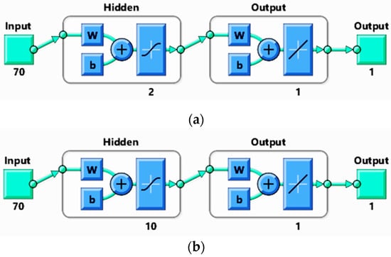
Figure 2.
Neural network diagrams used in this study: (a) using two hidden layers and (b) using 10 hidden layers. As input parameters, the four aforementioned clusters have been used.
Artificial neural networks have received considerable attention due to its powerful ability in image processing, natural language processing, etc. [78]. In this study, the Bayesian regularatzaion was used as a training algorithm of the neural network. The Bayesian framework allows the combination of uncertain and incomplete information with multi-source datasets, while it can provide a probabilistic information on the accuracy of the updated model [79]. The estimated parameters are modeled with random variables while their prior distribution is updated with data and observations to a posterior distribution through application of Bayes’ rule [79].
Once the BNN fusion models are estimated, their accuracy and performance is evalauted based on the MAE and R parameters (see Equations (3) and (4)) as well as the error historgams. Selected fused models, based on their performance, are then compared with the original GPR depth slices using several image quality indicators.
3. Results
3.1. Neural Netowork Regression Values
The results from the BNN using as inputs the first cluster—four multispectral bands—are depicted in Figure 3. The BNN model for the first depth slice (0.00–0.20 m below ground surface) has given a 0.50 regression value (R) as shown in Figure 3a. Similar regression values have also been reported in the rest depth slices (0.20–0.40 m and 0.40–0.60 m below ground surface) as shown in Figure 3b,c, respectively. R values are even lower when we fuse the GPR depth slices with individual vegetation indices from the second and third cluster. As shown in Figure 4, for the NDVI index (Table 1, no 1), R value is less than 0.40 (see Figure 4a,c) while for the depth slice between 0.20–0.40 m (Figure 4b) the R value is even less than 0.20. For the hyperspectral REP index (Table 2, no. 19) the R value results (Figure 5) are similar to the multispectral bands (Figure 3). It should be stated that these results are also in agreement to the linear regerssion models obtained from [5].
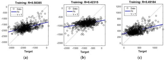
Figure 3.
BNN two hidden layers fitting results based on the 85% of the samples: (a) RGB-NIR bands against GPR slice depth between 0.00–0.20 m; (b) RGB-NIR bands against GPR slice depth between 0.20–0.40 m; and (c) RGB-NIR bands against GPR slice depth between 0.40–0.60 m.
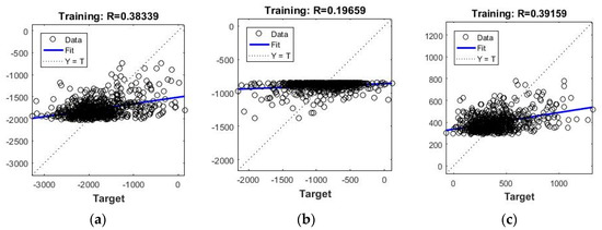
Figure 4.
BNN two hidden layers fitting results based on the 85% of the samples: (a) NDVI against GPR slice depth between 0.00–0.20 m; (b) NDVI against GPR slice depth between 0.20–0.40 m; and (c) NDVI against GPR slice depth between 0.40–0.60 m.
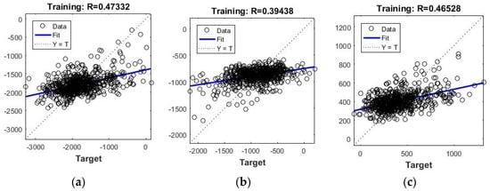
Figure 5.
BNN two hidden layers fitting results based on the 85% of the samples: (a) REP against GPR slice depth between 0.00–0.20 m; (b) REP against GPR slice depth between 0.20–0.40 m; and (c) REP against GPR slice depth between 0.40–0.60 m.
In our experiments, it was evident that no single vegetation index could sufficiently explain the GPR anomalies found in the various depth slices. This was also demonstrated in other studies focusing on the detection of buried features in optical remote sensing datasets based on crop marks [80,81]. To this end, the second, third and fourth clusters (i.e., multispectral vegetation indices, hyperspectral vegetation indices, and whole dataset respectivelly) was used.
The results obtained from the second cluster using the multispectral vegetation indices were similar with the first cluster (results in Figure 6). More specifically, the regression value was found to be 0.50, 0.41, and 0.41 for the depth slices 0.00–0.20 m, 0.20–0.40 m, and 0.40–0.60 m respectively. Even if these values are much more improved compared to the NDVI index (Figure 4), the results are not sufficient as the R value is still lower of 0.50.
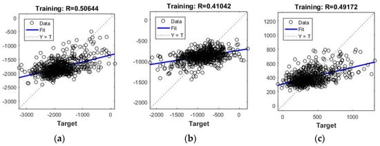
Figure 6.
BNN two hidden layers fitting results based on the 85% of the samples: (a) Group of multispectral vegetation indices against GPR slice depth between 0.00–0.20 m; (b) Group of multispectral vegetation indices against GPR slice depth between 0.20–0.40 m; and (c) Group of multispectral vegetation indices against GPR slice depth between 0.40–0.60 m.
In contrast, when the third cluster was used as input in the fusion model (i.e., hyperspectral vegetation indices), it was observed a major increased of the regression value; 0.67, 0.64, and 0.64 for the depth slices 0.00–0.20 m, 0.20–0.40 m, and 0.40–0.60 m below ground surface respectively (see Figure 7). Thus, hyperspectral indices provided more accurate fusion models between the ground spectral signatures and the GPR results. On the other hand, analysis based on the use of the whole dataset did not significantly improve these results as shown in Figure 8.
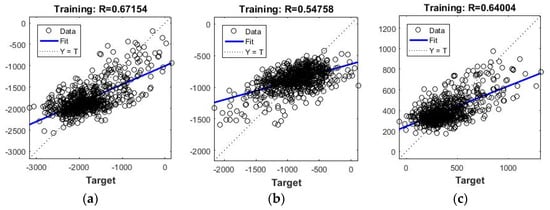
Figure 7.
BNN two hidden layers fitting results based on the 85% of the samples: (a) Group of hyperspectral vegetation indices against GPR slice depth between 0.00–0.20 m; (b) Group of hyperspectral vegetation indices against GPR slice depth between 0.20–0.40 m; and (c) Group of hyperspectral vegetation indices against GPR slice depth between 0.40–0.60 m.
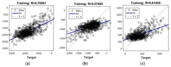
Figure 8.
BNN two hidden layers fitting results based on the 85% of the samples: (a) Group of multispectral bands, multispectral and hyperspectral vegetation indices against GPR slice depth between 0.00–0.20 m; (b) Group of multispectral bands, multispectral and hyperspectral vegetation indices against GPR slice depth between 0.20–0.40 m; and (c) Group of multispectral bands, multispectral and hyperspectral vegetation indices against GPR slice depth between 0.40–0.60 m.
In an effort to further investigate and improve the fusion model, the number of the hidden layers was increased from 2 to 10. The results using the whole dataset are shown in Figure 9. It is apparent that the overall regression values are quite high for the depth slices 0.00–0.20 m and 0.40–0.60 m (Figure 9a,c respectively) recording an R value higher than 0.80. However the results for the second depth slice 0.20–0.40 m are still poor with an R value of approximately 0.55. It is interesting and worth hightlighting that results with high regression values (more than 0.73) were found using 10 hidden layers and the hyperspectral vegetation indices (third cluster). These results are considered fairly sufficient for the fusion models between the spectral signatures and the GPR results for all the depth slices. The increased number of the hidden layers has increased the R value up to 0.20 in comparon to the results of Figure 7 and Figure 10 (10 and 2 hidden layers respectively). The regression values obtained in this study were also improved compared to the linear regression models tested in [5]. The higher regression values of [5] were 0.49, 0.38 and 0.47 using the REP index for the depth slices 0.00–0.20 m, 0.20–0.40 m, and 0.40–0.60 m below ground surface respectively. In this study, the results are 0.77, 0.73, and 0.80 (see Figure 10).
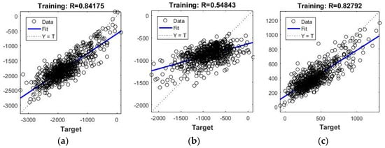
Figure 9.
BNN 10 hidden layers fitting results based on the 85% of the samples: (a) Group of multispectral bands, multispectral and hyperspectral vegetation indices against GPR slice depth between 0.00–0.20 m; (b) Group of multispectral bands, multispectral and hyperspectral vegetation indices against GPR slice depth between 0.20–0.40 m; and (c) Group of multispectral bands, multispectral and hyperspectral vegetation indices against GPR slice depth between 0.40–0.60 m.
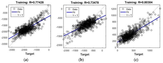
Figure 10.
BNN 10 hidden layers fitting results based on the 85% of the samples: (a) Group of hyperspectral vegetation indices against GPR slice depth between 0.00–0.20 m; (b) Group of hyperspectral vegetation indices against GPR slice depth between 0.20–0.40 m; and (c) Group of hyperspectral vegetation indices against GPR slice depth between 0.40–0.60 m.
3.2. Errors in Neural Netoworks
Various errors might occur in the fusing process of two different multi-instrument remotely sensed data. To avoid overfitted statistical models, the data were retrained several times using a random data division approach. As mentioned earlier, in our fusion models 85% of the data was used for training, while the rest 15% of the data was used for validation.
Beyond the regression value R, which is a numerical index of overall performance, the overall performance can be further monitored by the MAE and the training error diagrams. However, the interpretation of the MAE index can be problematic in cases like ours, where the global absolute error of the GPR signal is not so significant, since the signal value varies upon the case study area and the anomalies of the ground surface. Therefore, MAE index can be used during the training purposes along with the regression values as a proxy of good performance of the fusion model but not as an indicator of the quality of the specific fusion model trained for a specific archaeological site. In contrast, the distribution of the error (rather than the global error MAE) in the form of a histogram error (Figure 11), may be used not only for validation purposes, but also as a tool when interpreting the data after the application of the fusion model with other datasets.
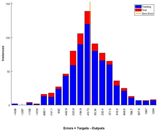
Figure 11.
Error histogram obtained after the application of BNN two hidden layers using the hyperspectral vegetation indices as an input parameter and the GPR slice depth between 0.00–0.20 m results as targets.
3.3. Comparison with Real GPR Slices
The overall performance of the fusion models was directly compared with the real GPR depth slices. For this task, the BNN fusion model generated using the hypespectral indices cluster, which provided high regression values for all three depth slices has been used. The application of the BNN fusion model was once again performed in the MATLAB environment. The GPR results acquired at the archaeological site of Vésztő-Mágor Tell—over the area shown in red polygon at Figure 1—are demonstrated in Figure 12a–c. The fused BNN results are shown in Figure 12d–f for the depth slices 0.00 up to 0.60 m. A linear horizontal feature exists at around 75–80 m north at all GPR depth slices (indicated with red arrow) up to a depth to 0.60 m. The same anomaly can be also observed in the BNN fused model (Figure 12d–f). Absolute differences (i.e., GPR results—BNN results) can be obviously reported between the real and the fused models (see results in Figure 13). These absolute differences are scattered accross the whole area of investigation, whereas no any specific pattern distribution can be seen for the three depth slices (Figure 13a–c).
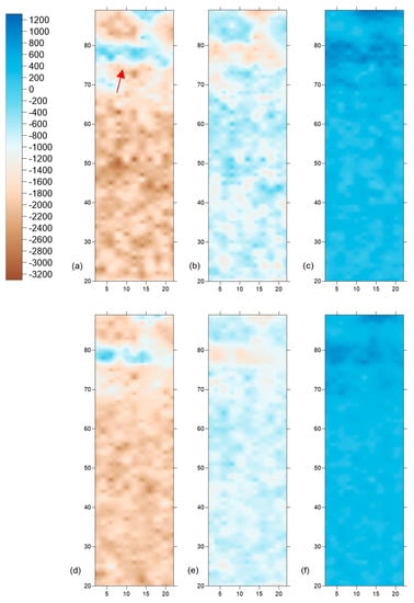
Figure 12.
GPR depth slices results for 0.00–0.20 m (a), 0.20–0.40 m (b), and 0.40–0.60 m (c) below ground surface and BNN fused results for 0.00–0.20 m (d), 0.20–0.40 m (e), and 0.40–0.60 m (f) below ground surface using the hyperspectral vegetation cluster. All depth slices have been rescaled to the same GPR amplitude range for consistency in the interpretation of the figure. High amplitude values are shown with blue color, while low amplitude values are shown with brown.
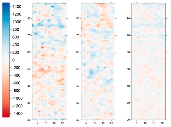
Figure 13.
Errors observed between the GPR in measurements (see Figure 12a–c) and the BNN fusion model (see Figure 12d–f) for the depth slices between 0.00–0.20 m (a), 0.20–0.40 m (b), and 0.40–0.60 m (c). Higher amplitude error values are shown with red colour while lower amplitude error values with blue.
The images generated from the GPR measurements and the BNN fused models (see Figure 12) were further analyzed using five different quality image methods: (a) bias, (b) image entropy, (c) ERGAS (erreur relative globale adimensionnelle de synthèse), (d) RASE (relative average spectral error), and (e) RMSE (root mean squared error). The equations for these image quality methods are given below (Equations. 5–9). More details regarding the details of the aforementioned quality image methods can be found in [82,83].
The results of the quality image methods are demonstrated in Figure 14. Each row of the figure represents a different depth slice: the first row refers to the depth slice 0.00–0.20 m, the second row refers to the depth slice 0.20–0.40 m, while the third row refers to the depth slice 0.40–0.60 m. Images are labelled as follow: (a) refers to the result after the bias, (b) to image entropy, (c) to ERGAS, (d) to RASE, and (e) to RMSE quality indices. The different quality indices indicate similar results for each depth, while the same observation can be made for the same index across the three depth slices. The main differences between the ‘real’ and the ‘modeled’ data are visible at the location of the linear feature.
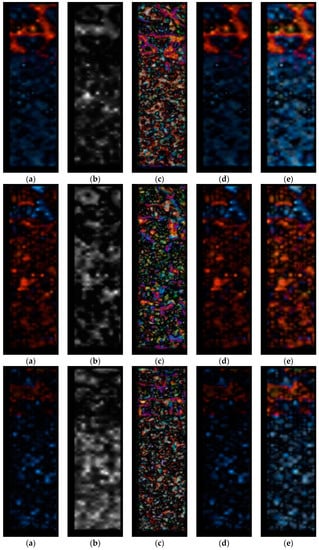
Figure 14.
Results from the (a) bias, (b) image entropy, (c) ERGAS (erreur relative globale adimensionnelle de synthèse), (d) RASE (relative average spectral error), and (e) RMSE (root mean squared error) quality image methods. The first row refers to the first depth slice (0.00–0.20 m), the second row to the 0.20–0.40 m depth slice and the third row to the 0.40–0.60 m depth slice. Red values represent higher mismatch between the ‘real’ image (GPR) and the ‘modeled’ image (BNN model) while blue color lower values. The radiometric scale of the images was set to 8 bit (0–255).
A quantitative analysis of the comparison between the real GPR measurements and the BNN fused datasets, are indicated in Table 3. Table 3 shows the results for the different quality image method used before (i.e., bias, entropy, ERGAS, RASE, and RMSE) for different depths (i.e., 0.00–0.20 m, 0.20–0.40 m, and 0.40–0.60 m below surface). Values close to zero (0) are considered ideal, since the fused images results are matched with the real GPR datasets. Based on these results, it is important to highlight the fact that layers 0.20–0.40 m and 0.40–0.60 m below surface seem to provide slightly more ‘realistic’ results compared to the upper layer, as indicated for instance for the bias method (0.11 for layer 0.00–0.20 m, 0.06 for layer 0.20–0.40 m, and 0.08 for layer 0.40–0.60 m below surface). The layer 0.20–0.40 m provide the best results for all quality image methods examined providing average results of 0.06, 0.59, 1.80, 7.43, and 13.75 for bias, entropy, ERGAS, RASE, and RMSE methods respectively.
Table 3.
Quantitative Analysis of original GPR results with the fused image results through BNN application in different levels.
4. Discussion
In the recent years, advances in remote sensing have shown its potential strengths in archaeological research [84,85,86]. Despite these new technological improvements in terms of spatial, spectral and temporal resolution, the combination and fusion of different types of remotely sensed data is still open for research. Fusion of different datasets can further explore the way we interpret remotely sensed data for archaeological research. In this study, ground sensors (i.e., GPR and spectroradiometer) were used to examine potential correlation between the two datasets. Based on the results demonstrated in the previous section, recent advancements in machine learning for image analysis, such as neural networks, can establish high correlation coefficient (>0.70) between the datasets. This correlation has been relative increased by 40% compared to the findings of previous studies [5]. In study [5], the best results were reported using the REP index with a correlation coefficient value ranging from 0.38–0.49. One important aspect found in this study is the ability of the neural networks to produce high correlation coefficient regression models for all the upper layers of soil (i.e., for layer 0.00–0.20 m, 0.20–0.40 m, and 0.40–0.60 m below surface).
Once a high correlation between the two different datasets is achieved then the established BNN model, i.e., from GPR to optical remote sensed datasets, enables us to ‘transfer’ the model to optical remotely sensed data in various depth slices. The results also indicated that aerial and low altitude hyperspectral datasets can be considered as ideal for similar investigations as proposed in this study due to their ability to provide not only high spatial resolution images but also due to the higher correlation coefficient of the regression models in contrast to multispectral sensors.
In this way, hyperspectral datasets can be trained to ‘predict’ GPR depth slices up to a depth of 0.60 m below ground surface and therefore identify hot-spot areas. The model does not follow a supervised approach, i.e., firstly to identify and extract archaeological features from the GPR dataset and then to apply the model, but rather to model the entire area of investigation between the two different datasets. Significant variability in the R values obtained in different depth slices can also lead to errors and misleading. Of course, this is impossible to predict since it needs to be assumed that soil and vegetation characteristics along with archeological features’ properties are uniform across the study area (but not necessarily spatially uniform).
Of course, this predictive model should be further investigated, improved, and incorporate new insights from on-going archaeological excavations, other geophysical prospection datasets, etc. However, the propose method enable us to re-use the numerous archived hyperspectral datasets from airborne campaigns blended with ground geophysical prospection data. The results from this experiment demonstrated that this fusion model is feasible, with unavoidable differences between the ‘real’ and the ‘modeled’ data. It should be also stressed that the fused model is reliable in areas with similar context (i.e., archaeological and environmental context), therefore a prior knowledge of the area of interest in essential.
An overall methodology of the proposed work is demonstrated in following Figure 15. The various steps include the collection of the ground datasets (GPR and ground spectroradiometric measurements) over the same area and their pre-processing steps for noise removal and co-registration of the data. It should be mentioned that the collection of the ground datasets should be carried out almost simultaneously so as to minimize any phenological changes of the crops and soil moisture levels. Then various multispectral and hyperspectral indices can estimate using the ground spectral signatures as these are described in Table 1 and Table 2. The next step includes the fusion modeling between the vegetation indices and the different depth slices based on BNN. The results are then evaluated and compared with the in-situ GPR measurements. This step is of high importance since it will assess the overall performance of the fused model with the different GPR slices. Once the fused model is acceptable, then this can be applied to satellite image.
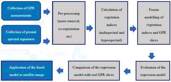
Figure 15.
Overall methodology of the proposed work.
5. Conclusions
This paper presents the results from an ongoing research oriented towards the fusion of multi-source and multi-instrument remote sensing datasets acquired for archaeological applications. This study aims to push research towards new ways of exploiting different remote sensing data, through the integration and fusion of them. For this purpose, archive GPR and ground spectral signature data have been acquired and processed using Bayesian neural network models.
The results have shown that hyperspectral vegetation indices can be strongly correlated with the GPR results for the upper layers of ground surface (i.e., up to a depth of 0.60 m) providing a statistical correlation coefficient of more than 0.73 for all depth slices. Even though defining a threshold to R value for providing a strong correlation between the different datasets is difficult—since each case study has its own characteristics—an R value of more than 0.70 is considered a good starting point. The BNN fusion results have also been compared, using various ways, with the initial GPR measurements. The fused models were able to detect the linear feature originally detected by the GPR, at all the shallow depth slices.
Potential errors and overfitting models have also been discussed in this paper. Of course, as already mentioned earlier, the use of remote sensing data and their interpretation for archaeological mapping “is not without risks and challenges” [1]. Further investigation is needed since the fused models are sensitive to the study area and need to be adjusted for each site in order to preserve as much information as possible.
Our approach can be potentially used in two ways: (a) firstly, someone may re-use archived geophysical prospection data and blend them with optical remote sensing datasets (either aerial or space, including drone sensors) and (b) secondly, somebody may ‘predict’ (model) priority areas based on geophysical or other remotely sensed data for further non-contact remote sensing techniques. Of course, high correlation achieved between the different datasets is reliable only for similar soil characteristics and targets (i.e., archaeological features). Future work may be focused on other areas with different soil conditions and underneath targets in order to further explore the feasibility of this methodology.
Author Contributions
Conceptualization and Methodology, A.A., Data Analysis AA., A.S., Writing—Original Draft Preparation, A.A.; Writing—Review & Editing, A.S.
Funding
This research received no external funding.
Acknowledgments
The fieldwork campaign was supported by USA-NSF (U.S.-Hungarian-Greek Collaborative International Research Experience for Students on Origins and Development of Prehistoric European Villages) and Wenner-Gren Foundation (International Collaborative Research Grant, “Early Village Social Dynamics: Prehistoric Settlement Nucleation on The Great Hungarian Plain”). William A. Parkinson, Richard W. Yerkes, Attila Gyucha, and Paul R. Duffy provided their expertise and support in the fieldwork activities. The authors would like also to thank D.G. Hadjimitsis for his support, as well as the Eratosthenes Research Center of the Cyprus University of Technology. Thanks are also given to Milto Miltiadou of the same university for her grammar editing and comments. The authors would like also to acknowledge the “CUT Open Access Author Fund” for covering the open access publication fees of the paper.
Conflicts of Interest
The authors declare no conflict of interest.
References
- Banaszek, Ł.; Cowley, D.C.; Middleton, M. Towards National Archaeological Mapping. Assessing Source Data and Methodology—A Case Study from Scotland. Geosciences 2018, 8, 272. [Google Scholar] [CrossRef]
- Opitz, R.; Herrmann, J. Recent Trends and Long-standing Problems in Archaeological Remote Sensing. J. Comput. Appl. Archaeol. 2018, 1, 19–41. [Google Scholar] [CrossRef]
- Leisz, S.J. An overview of the application of remote sensing to archaeology during the twentieth century. In Mapping Archaeological Landscapes from Space; Springer: New York, NY, USA, 2013; pp. 11–19. [Google Scholar]
- Filzwieser, R.; Olesen, L.H.; Verhoeven, G.; Mauritsen, E.S.; Neubauer, W.; Trinks, I.; Nowak, M.; Nowak, R.; Schneidhofer, P.; Nau, E.; et al. Integration of Complementary Archaeological Prospection Data from a Late Iron Age Settlement at Vesterager—Denmark. J. Archaeol. Method Theory 2018, 25, 313–333. [Google Scholar] [CrossRef]
- Agapiou, A.; Lysandrou, V.; Sarris, A.; Papadopoulos, N.; Hadjimitsis, D.G. Fusion of Satellite Multispectral Images Based on Ground-Penetrating Radar (GPR) Data for the Investigation of Buried Concealed Archaeological Remains. Geosciences 2017, 7, 40. [Google Scholar] [CrossRef]
- Gharbia, R.; Hassanien, A.E.; El-Baz, A.H.; Elhoseny, M.; Gunasekaran, M. Multi-spectral and panchromatic image fusion approach using stationary wavelet transform and swarm flower pollination optimization for remote sensing applications. Future Gener. Comput. Syst. 2018, 88, 501–511. [Google Scholar] [CrossRef]
- Alexakis, D.; Sarris, A.; Astaras, T.; Albanakis, Κ. Detection of neolithic settlements in thessaly (Greece) through multispectral and hyperspectral satellite imagery. Sensors 2009, 9, 1167–1187. [Google Scholar] [CrossRef] [PubMed]
- Alexakis, A.; Sarris, A.; Astaras, T.; Albanakis, K. Integrated GIS, remote sensing and geomorphologic approaches for the reconstruction of the landscape habitation of Thessaly during the Neolithic period. J. Archaeol. Sci. 2011, 38, 89–100. [Google Scholar] [CrossRef]
- Traviglia, A.; Cottica, D. Remote sensing applications and archaeological research in the Northern Lagoon of Venice: The case of the lost settlement of Constanciacus. J. Archaeol. Sci. 2011, 38, 2040–2050. [Google Scholar] [CrossRef]
- Gallo, D.; Ciminale, M.; Becker, H.; Masini, N. Remote sensing techniques for reconstructing a vast Neolithic settlement in Southern Italy. J. Archaeol. Sci. 2009, 36, 43–50. [Google Scholar] [CrossRef]
- Yu, L.; Zhang, Y.; Nie, Y.; Zhang, W.; Gao, H.; Bai, X.; Liu, F.; Hategekimana, Y.; Zhu, J. Improved detection of archaeological features using multi-source data in geographically diverse capital city sites. J. Cult. Herit. 2018, 33, 145–158. [Google Scholar] [CrossRef]
- Nsanziyera, F.A.; Lechgar, H.; Fal, S.; Maanan, M.; Saddiqi, O.; Oujaa, A.; Rhinane, H. Remote-sensing data-based Archaeological Predictive Model (APM) for archaeological site mapping in desert area, South Morocco. C. R. Geosci. 2018, 350, 319–330. [Google Scholar] [CrossRef]
- Morehart, T.C.; Millhauser, K.J. Monitoring cultural landscapes from space: Evaluating archaeological sites in the Basin of Mexico using very high resolution satellite imagery. J. Archaeol. Sci. Rep. 2016, 10, 363–376. [Google Scholar] [CrossRef]
- Lasaponara, R.; Masini, N. Beyond modern landscape features: New insights in the archaeological area of Tiwanaku in Bolivia from satellite data. Int. J. Appl. Earth Obs. Geoinform. 2014, 26, 464–471. [Google Scholar] [CrossRef]
- Agapiou, A.; Lysandrou, V.; Hadjimitsis, D.G. Optical Remote Sensing Potentials for Looting Detection. Geosciences 2017, 7, 98. [Google Scholar] [CrossRef]
- Di Maio, R.; La Manna, M.; Piegari, E.; Zara, A.; Bonetto, J. Reconstruction of a Mediterranean coast archaeological site by integration of geophysical and archaeological data: The eastern district of the ancient city of Nora (Sardinia, Italy). J. Archaeol. Sci. Rep. 2018, 20, 230–238. [Google Scholar] [CrossRef]
- Balkaya, Ç.; Kalyoncuoğlu, Ü.Y.; Özhanlı, M.; Merter, G.; Çakmak, O.; Talih Güven, İ. Ground-penetrating radar and electrical resistivity tomography studies in the biblical Pisidian Antioch city, southwest Anatolia. Archaeol. Prospect. 2018, 1–16. [Google Scholar] [CrossRef]
- Küçükdemirci, M.; Özer, E.; Piro, S.; Baydemir, N.; Zamuner, D. An application of integration approaches for archaeo-geophysical data: Case study from Aizanoi. Archaeol. Prospect. 2018, 25, 33–44. [Google Scholar] [CrossRef]
- Gustavsen, L.; Cannell, R.J.S.; Nau, E.; Tonning, C.; Trinks, I.; Kristiansen, M.; Gabler, M.; Paasche, K.; Gansum, T.; Hinterleitner, A.; et al. Archaeological prospection of a specialized cooking-pit site at Lunde in Vestfold, Norway. Archaeol. Prospect. 2018, 25, 17–31. [Google Scholar] [CrossRef]
- Bevan, A. The data deluge. Antiquity 2015, 89, 1473–1484. [Google Scholar] [CrossRef]
- Orengo, H.; Petrie, C. Large-Scale, Multi-Temporal Remote Sensing of Palaeo-River Networks: A Case Study from Northwest India and its Implications for the Indus Civilisation. Remote Sens. 2017, 9, 735. [Google Scholar] [CrossRef]
- Agapiou, A. Remote sensing heritage in a petabyte-scale: Satellite data and heritage Earth Engine© applications. Int. J. Digit. Earth 2017, 10, 85–102. [Google Scholar] [CrossRef]
- Liss, B.; Howland, D.M.; Levy, E.T. Testing Google Earth Engine for the automatic identification and vectorization of archaeological features: A case study from Faynan, Jordan. J. Archaeol. Sci. Rep. 2017, 15, 299–304. [Google Scholar] [CrossRef]
- Gyucha, A.; Yerkes, W.R.; Parkinson, A.W.; Sarris, A.; Papadopoulos, N.; Duffy, R.P.; Salisbury, B.R. Settlement Nucleation in the Neolithic: A Preliminary Report of the Körös Regional Archaeological Project’s Investigations at Szeghalom-Kovácshalom and Vésztő-Mágor. In Neolithic and Copper Age between the Carpathians and the Aegean Sea: Chronologies and Technologies from the 6th to the 4th Millennium BCE; Hansen, S., Raczky, P., Anders, A., Reingruber, A., Eds.; International Workshop Budapest 2012; Dr. Rudolf Habelt: Bonn, Germany, 2012; pp. 129–142. [Google Scholar]
- Hegedűs, K. Vésztő-Mágori-domb. In Magyarország Régészeti Topográfiája VI; Ecsedy, I., Kovács, L., Maráz, B., Torma, I., Eds.; Békés Megye Régészeti Topográfiája: A Szeghalmi Járás 1982 IV/1; Akadémiai Kiadó: Budapest, Hungary, 1982; pp. 184–185. [Google Scholar]
- Hegedűs, K.; Makkay, J. Vésztő-Mágor: A Settlement of the Tisza Culture. In The Late Neolithic of the Tisza Region: A Survey of Recent Excavations and Their Findings; Tálas, L., Raczky, P., Eds.; Szolnok County Museums: Szolnok, Hungary, 1987; pp. 85–104. [Google Scholar]
- Makkay, J. Vésztő–Mágor. In Ásatás a Szülőföldön; Békés Megyei Múzeumok Igazgatósága: Békéscsaba, Hungary, 2004. [Google Scholar]
- Parkinson, W.A. Tribal Boundaries: Stylistic Variability and Social Boundary Maintenance during the Transition to the Copper Age on the Great Hungarian Plain. J. Anthropol. Archaeol. 2006, 25, 33–58. [Google Scholar] [CrossRef]
- Juhász, I. A Csolt nemzetség monostora. In A középkori Dél-Alföld és Szer; Kollár, T., Ed.; Csongrád Megyei Levéltár: Szeged, Hungary, 2000; pp. 281–304. [Google Scholar]
- Sarris, A.; Papadopoulos, N.; Agapiou, A.; Salvi, M.C.; Hadjimitsis, D.G.; Parkinson, A.; Yerkes, R.W.; Gyucha, A.; Duffy, R.P. Integration of geophysical surveys, ground hyperspectral measurements, aerial and satellite imagery for archaeological prospection of prehistoric sites: The case study of Vészt˝o-Mágor Tell, Hungary. J. Archaeol. Sci. 2013, 40, 1454–1470. [Google Scholar] [CrossRef]
- Agapiou, A.; Sarris, A.; Papadopoulos, N.; Alexakis, D.D.; Hadjimitsis, D.G. 3D pseudo GPR sections based on NDVI values: Fusion of optical and active remote sensing techniques at the Vészto-Mágor tell, Hungary. In Archaeological Research in the Digital Age, Proceedings of the 1st Conference on Computer Applications and Quantitative Methods in Archaeology Greek Chapter (CAA-GR), Rethymno Crete, Greece, 6–8 March 2014; Papadopoulos, C., Paliou, E., Chrysanthi, A., Kotoula, E., Sarris, A., Eds.; Institute for Mediterranean Studies-Foundation of Research and Technology (IMS-Forth): Rethymno, Greece, 2015. [Google Scholar]
- Agapiou, A. Development of a Novel Methodology for the Detection of Buried Archaeological Remains Using Remote Sensing Techniques. Ph.D. Thesis, Cyprus University of Technology, Limassol, Cyprus, 2012. (In Greek). Available online: http://ktisis.cut.ac.cy/handle/10488/6950 (accessed on 7 November 2018).
- Neal, R.M. Bayesian Learning for Neural Networks; Springer Science & Business Media: New York, NY, USA, 2012; p. 118. [Google Scholar]
- Rouse, J.W.; Haas, R.H.; Schell, J.A.; Deering, D.W.; Harlan, J.C. Monitoring the Vernal Advancements and Retrogradation (Greenwave Effect) of Nature Vegetation; NASA/GSFC Final Report; NASA: Greenbelt, MD, USA, 1974. [Google Scholar]
- Roujean, J.L.; Breon, F.M. Estimating PAR absorbed by vegetation from bidirectional reflectance measurements. Remote Sens. Environ. 1995, 51, 375–384. [Google Scholar] [CrossRef]
- Gamon, J.A.; Surfus, J.S. Assessing leaf pigment content and activity with a reflectometer. New Phytol. 1999, 143, 105–117. [Google Scholar] [CrossRef]
- Richardson, A.J.; Wiegand, C.L. Distinguishing vegetation from soil background information. Photogramm. Eng. Remote Sens. 1977, 43, 15–41. [Google Scholar]
- Pearson, R.L.; Miller, L.D. Remote Mapping of Standing Crop Biomass and Estimation of the Productivity of the Short Grass Prairie, Pawnee National Grasslands, Colorado. In Proceedings of the 8th International Symposium on Remote Sensing of the Environment, Ann Arbor, MI, USA, 2–6 October 1972; pp. 1357–1381. [Google Scholar]
- Baret, F.; Guyot, G. Potentials and limits of vegetation indices for LAI and APAR assessment. Remote Sens. Environ. 1991, 35, 161–173. [Google Scholar] [CrossRef]
- Qi, J.; Chehbouni, A.; Huete, A.R.; Kerr, Y.H.; Sorooshian, S. A modified soil adjusted vegetation index. Remote Sens. Environ. 1994, 48, 119–126. [Google Scholar] [CrossRef]
- Kaufman, Y.J.; Tanré, D. Atmospherically resistant vegetation index (ARVI) for EOS-MODIS. IEEE Trans. Geosci. Remote Sens. 1992, 30, 261–270. [Google Scholar] [CrossRef]
- Pinty, B.; Verstraete, M.M. GEMI: A non-linear index to monitor global vegetation from satellites. Plant Ecol. 1992, 101, 15–20. [Google Scholar] [CrossRef]
- Rondeaux, G.; Steven, M.; Baret, F. Optimization of soil-adjusted vegetation indices. Remote Sens. Environ. 1996, 55, 95–107. [Google Scholar] [CrossRef]
- Tucker, C.J. Red and photographic infrared linear combinations for monitoring vegetation. Remote Sens. Environ. 1979, 8, 127–150. [Google Scholar] [CrossRef]
- Gong, P.; Pu, R.; Biging, G.S.; Larrieu, M.R. Estimation of forest leaf area index using vegetation indices derived from Hyperion hyperspectral data. IEEE Trans. Geosci. Remote Sens. 2003, 41, 1355–1362. [Google Scholar] [CrossRef]
- Kim, M.S.; Daughtry, C.S.T.; Chappelle, E.W.; McMurtrey, J.E., III; Walthall, C.L. The Use of High Spectral Resolution Bands for Estimating Absorbed Photosynthetically Active Radiation (APAR). In Proceedings of the 6th Symposium on Physical Measurements and Signatures in Remote Sensing, Val D’Isere, France, 17–21 January 1994. [Google Scholar]
- Zarco-Tejada, P.J.; Berjón, A.; López-Lozano, R.; Miller, J.R.; Martín, P.; Cachorro, V.; González, M.R.; de Frutos, A. Assessing vineyard condition with hyperspectral indices: Leaf and canopy reflectance simulation in a row-structured discontinuous canopy. Remote Sens. Environ. 2005, 99, 271–287. [Google Scholar] [CrossRef]
- Gandia, S.; Fernández, G.; García, J.C.; Moreno, J. Retrieval of Vegetation Biophysical Variables from CHRIS/PROBA Data in the SPARC Campaing. In Proceedings of the 4th ESA CHRIS PROBA Workshop, Frascati, Italy, 28–30 April 2004; pp. 40–48. [Google Scholar]
- Daughtry, C.S.T.; Walthall, C.L.; Kim, M.S.; de Colstoun, E.B.; McMurtrey, J.E. Estimating corn leaf chlorophyll concentration from leaf and canopy reflectance. Remote Sens. Environ. 2000, 74, 229–239. [Google Scholar] [CrossRef]
- Haboudane, D.; Miller, J.R.; Pattey, E.; Zarco-Tejada, P.J.; Strachan, I. Hyperspectral vegetation indices and novel algorithms for predicting green LAI of crop canopies: Modeling and validation in the context of precision agriculture. Remote Sens. Environ. 2004, 90, 337–352. [Google Scholar] [CrossRef]
- Sims, D.A.; Gamon, J.A. Relationships between leaf pigment content and spectral reflectance across a wide range of species, leaf structures and developmental stages. Remote Sens. Environ. 2002, 81, 337–354. [Google Scholar] [CrossRef]
- Castro-Esau, K.L.; Sánchez-Azofeifa, G.A.; Rivard, B. Comparison of spectral indices obtained using multiple spectroradiometers. Remote Sens. Environ. 2006, 103, 276–288. [Google Scholar] [CrossRef]
- Chen, J.; Cihlar, J. Retrieving leaf area index of boreal conifer forests using Landsat Thematic Mapper. Remote Sens. Environ. 1996, 55, 153–162. [Google Scholar] [CrossRef]
- Dash, J.; Curran, P.J. The MERIS terrestrial chlorophyll index. Int. J. Remote Sens. 2004, 25, 5403–5413. [Google Scholar] [CrossRef]
- Gitelson, A.; Merzlyak, M.N. Quantitative estimation of chlorophyll-a using reflectance spectra: Experiments with autumn chestnut and maple leaves. J. Photochem. Photobiol. B Biol. 1994, 22, 247–252. [Google Scholar] [CrossRef]
- Guyot, G.; Baret, F.; Major, D.J. High spectral resolution: Determination of spectral shifts between the red and near infrared. Int. Arch. Photogramm. Remote Sens. Spat. Inf. Sci. 1988, 11, 750–760. [Google Scholar]
- Peñuelas, J.; Filella, I.; Lloret, P.; Munoz, F.; Vilajeliu, M. Reflectance assessment of mite effects on apple trees. Int. J. Remote Sens. 1995, 16, 2727–2733. [Google Scholar] [CrossRef]
- Penuelas, J.; Baret, F.; Filella, I. Semi-empirical indices to assess carotenoids/chlorophyll-a ratio from leaf spectral reflectance. Photosynthetica 1995, 31, 221–230. [Google Scholar]
- Vincini, M.; Frazzi, E.; D’Alessio, P. Angular Dependence of Maize and Sugar Beet Vis from Directional CHRIS/PROBA Data. In Proceedings of the 4th ESA CHRIS PROBA Workshop, Frascati, Italy, 19–21 September 2006; pp. 19–21. [Google Scholar]
- Jordan, C.F. Derivation of leaf area index from quality of light on the forest floor. Ecology 1969, 50, 663–666. [Google Scholar] [CrossRef]
- Gitelson, A.A.; Merzlyak, M.N. Remote estimation of chlorophyll content in higher plant leaves. Int. J. Remote Sens. 1997, 18, 2691–2697. [Google Scholar] [CrossRef]
- Datt, B. Remote sensing of chlorophyll a, chlorophyll b, chlorophyll a+b, and total carotenoid content in eucalyptus leaves. Remote Sens. Environ. 1998, 66, 111–121. [Google Scholar] [CrossRef]
- Haboudane, D.; Miller, J.R.; Tremblay, N.; Zarco-Tejada, P.J.; Dextraze, L. Integrated narrow-band vegetation indices for prediction of crop chlorophyll content for application to precision agriculture. Remote Sens. Environ. 2002, 81, 416–426. [Google Scholar] [CrossRef]
- Broge, N.H.; Leblanc, E. Comparing prediction power and stability of broadband and hyperspectral vegetation indices for estimation of green leaf area index and canopy chlorophyll density. Remote Sens. Environ. 2001, 76, 156–172. [Google Scholar] [CrossRef]
- Vogelmann, J.E.; Rock, B.N.; Moss, D.M. Red edge spectral measurements from sugar maple leaves. Int. J. Remote Sens. 1993, 14, 1563–1575. [Google Scholar] [CrossRef]
- Zarco-Tejada, P.J.; Pushnik, J.C.; Dobrowski, S.; Ustin, S.L. Steady-state chlorophyll a fluorescence detection from canopy derivative reflectance and double-peak red-edge effects. Remote Sens. Environ. 2003, 84, 283–294. [Google Scholar] [CrossRef]
- Gitelson, A.A.; Merzlyak, M.N.; Chivkunova, O.B. Optical properties and nondestructive estimation of anthocyanin content in plant leaves. Photochem. Photobiol. 2001, 74, 38–45. [Google Scholar] [CrossRef]
- Gitelson, A.A.; Zur, Y.; Chivkunova, O.B.; Merzlyak, M.N. Assessing carotenoid content in plant leaves with reflectance spectroscopy. Photochem. Photobiol. 2002, 75, 272–281. [Google Scholar] [CrossRef]
- Lichtenthaler, H.K.; Lang, M.; Sowinska, M.; Heisel, F.; Miehe, J.A. Detection of vegetation stress via a new high resolution fluorescence imaging system. J. Plant Physiol. 1996, 148, 599–612. [Google Scholar] [CrossRef]
- Peñuelas, J.; Gamon, J.A.; Fredeen, A.L.; Merino, J.; Field, C.B. Reflectance indices associated with physiological changes in nitrogen- and water-limited sunflower leaves. Remote Sens. Environ. 1994, 48, 135–146. [Google Scholar] [CrossRef]
- Barnes, J.D.; Balaguer, L.; Manrique, E.; Elvira, S.; Davison, A.W. A reappraisal of the use of DMSO for the extraction and determination of chlorophylls a and b in lichens and higher plants. Environ. Exp. Bot. 1992, 32, 85–100. [Google Scholar] [CrossRef]
- Gamon, J.A.; Serrano, L.; Surfus, J.S. The photochemical reflectance index: An optical indicator of photosynthetic radiation use efficiency across species, functional types, and nutrient levels. Oecologia 1997, 112, 492–501. [Google Scholar] [CrossRef] [PubMed]
- Filella, I.; Amaro, T.; Araus, J.L.; Peñuelas, J. Relationship between photosynthetic radiation-use efficiency of barley canopies and the photochemical reflectance index (PRI). Physiol. Plant. 1996, 96, 211–216. [Google Scholar] [CrossRef]
- Merzlyak, M.N.; Gitelson, A.A.; Chivkunova, O.B.; Rakitin, V.Y. Nondestructive optical detection of pigment changes during leaf senescence and fruit ripening. Physiol. Plant. 1999, 106, 135–141. [Google Scholar] [CrossRef]
- White, D.C.; Williams, M.; Barr, S.L. Detecting sub-surface soil disturbance using hyperspectral first derivative band rations of associated vegetation stress. Int. Arch. Photogramm. Remote Sens. Spat. Inf. Sci. 2008, 27, 243–248. [Google Scholar]
- Peñuelas, J.; Filella, I.; Biel, C.; Serrano, L.; Savé, R. The reflectance at the 950–970 nm region as an indicator of plant water status. Int. J. Remote Sens. 1993, 14, 1887–1905. [Google Scholar] [CrossRef]
- Gnana Sheela, K.; Deepa, S.N. Review on Methods to Fix Number of Hidden Neurons in Neural Networks. Math. Probl. Eng. 2013, 2013, 425740. [Google Scholar] [CrossRef]
- Cao, W.; Wang, X.; Ming, Z.; Gao, J. A review on neural networks with random weights. Neurocomputing 2018, 275, 278–287. [Google Scholar] [CrossRef]
- Giovanis, G.D.; Papaioannou, I.; Straub, D.; Papadopoulos, V. Bayesian updating with subset simulation using artificial neural networks. Comput. Methods Appl. Mech. Eng. 2017, 319, 124–145. [Google Scholar] [CrossRef]
- Cerra, D.; Agapiou, A.; Cavalli, R.M.; Sarris, A. An Objective Assessment of Hyperspectral Indicators for the Detection of Buried Archaeological Relics. Remote Sens. 2018, 10, 500. [Google Scholar] [CrossRef]
- Agapiou, A.; Hadjimitsis, D.G.; Alexakis, D.D. Evaluation of Broadband and Narrowband Vegetation Indices for the Identification of Archaeological Crop Marks. Remote Sens. 2012, 4, 3892–3919. [Google Scholar] [CrossRef]
- Ghassemian, H. A review of remote sensing image fusion methods. Inf. Fusion 2016, 32 Pt A, 75–89. [Google Scholar] [CrossRef]
- Vaiopoulos, A.D. Developing Matlab scripts for image analysis and quality assessment. In Proceedings of the SPIE 8181, Earth Resources and Environmental Remote Sensing/GIS Applications II, 81810B, Prague, Czech Republic, 26 October 2011. [Google Scholar] [CrossRef]
- Agapiou, A.; Lysandrou, V. Remote sensing archaeology: Tracking and mapping evolution in European scientific literature from 1999 to 2015. J. Archaeol. Sci. Rep. 2015, 4, 192–200. [Google Scholar] [CrossRef]
- Tapete, D.; Cigna, F. Trends and perspectives of space-borne SAR remote sensing for archaeological landscape and cultural heritage applications. J. Archaeol. Sci. Rep. 2017, 14, 716–726. [Google Scholar] [CrossRef]
- Chen, F.; Lasaponara, R.; Masini, N. An overview of satellite synthetic aperture radar remote sensing in archaeology: From site detection to monitoring. J. Cult. Herit. 2017, 23, 5–11. [Google Scholar] [CrossRef]
© 2018 by the authors. Licensee MDPI, Basel, Switzerland. This article is an open access article distributed under the terms and conditions of the Creative Commons Attribution (CC BY) license (http://creativecommons.org/licenses/by/4.0/).