Abstract
Parametric cyclonic wind fields are widely used worldwide for insurance risk underwriting, coastal planning, and storm surge forecasts. They support high-stakes financial, development and emergency decisions. Yet, there is still no consensus on a potentially “best” parametric approach, nor guidance to choose among the great variety of published models. The aim of this paper is to demonstrate that recent progress in estimating extreme surface wind speeds from satellite remote sensing now makes it possible to assess the performance of existing parametric models, and select a relevant one with greater objectivity. In particular, we show that the Cyclone Global Navigation Satellite System (CYGNSS) mission of NASA, along with the Advanced Scatterometer (ASCAT), are able to capture a substantial part of the tropical cyclone structure, and to aid in characterizing the strengths and weaknesses of a number of parametric models. Our results suggest that none of the traditional empirical approaches are the best option in all cases. Rather, the choice of a parametric model depends on several criteria, such as cyclone intensity and the availability of wind radii information. The benefit of using satellite remote sensing data to select a relevant parametric model for a specific case study is tested here by simulating hurricane Maria (2017). The significant wave heights computed by a wave-current hydrodynamic coupled model are found to be in good agreement with the predictions given by the remote sensing data. The results and approach presented in this study should shed new light on how to handle parametric cyclonic wind models, and help the scientific community conduct better wind, wave, and surge analyses for tropical cyclones.
Keywords:
CYGNSS; ASCAT; cyclones; hurricanes; parametric models; storm surges; waves; winds; remote sensing 1. Introduction
Since the overview of Vickery et al. [1], numerical atmospheric models have been increasingly applied in storm surge prediction and coastal hazard assessment studies [2,3,4,5]. Nonetheless, parametric models deriving cyclonic wind fields from a few input parameters (pressure drop, maximum velocity, wind radii, location of the cyclone center, etc.) are still widely used by the research and insurance communities, due to their simplicity, efficiency, and low-computational cost [6,7,8,9,10,11,12]. This is especially true for studies investigating storm surge hazards with statistical approaches, for which a large number of synthetic storms need to be represented [13,14,15,16].
For a few decades (and even today), the parametric surface winds have simply been derived as the sum of an axisymmetric wind field and a uniform vector to mimic the asymmetry due to the storm’s translational motion. Debates have arisen to determine the best way to estimate both components, which is a particularly relevant issue, as large discrepancies of the synthesized wind field occur depending on the chosen method [17]. This kind of approach, in which the tropical cyclone (TC) size is generally determined by a single parameter, the radius of maximum winds, presents several limitations. In particular, it does not always satisfactorily represent the TC wind asymmetry, which can be due to many factors, such as a blocking action by a neighboring anticyclone, boundary layer friction, or terrestrial effects [18].
To date, the increasing availability of satellite remote sensing data makes it possible to better depict and forecast the wind structure of TCs and its variations with azimuth. Whether based on infrared imagery and data [19,20,21], scatterometry [22,23], X-band, C-band and L-band radiometry [24,25,26,27,28,29], or global navigation satellite system-reflectometry (GNSS-R) [30,31,32], all these data can provide information about the 34-kt, 50-kt, and/or 64-kt wind radii in each TC quadrant. These radii are now commonly reported in advisories issued by warning centers.
Yet, to our knowledge, few studies investigating TC winds, cyclonic-induced waves, or storm surges using parametric models make use of all the available information, whether for forecasts or hindcasts. Often, only the estimated radius of maximum winds or the 64-kt wind radius is used, which can lead to systematic errors in the extended wind field. Additionally, there is little guidance to help choose a relevant gradient wind model, i.e., a parametric model that is expected to accurately represent the increase and decay of wind speed as a function of distance from the TC center. One example of this is the Holland [33] vortex. Although known to have significant limitations [34], this model is still widely used by the research and insurance communities worldwide. Other commonly used parametric wind models (for which there is room for improvement) include, for example, those by Jelesnianski and Taylor [35] and Emanuel and Rotunno [36]. New models are frequently proposed [18,37], but no consensus has been reached in favor of any one of them.
The difficulty in choosing among the great variety of gradient wind profiles can be attributed to a number of factors, including the fact that:
- Validations of parametric wind models are generally performed using a limited number of “ground-truth” data. In-situ observations of surface wind speeds are relatively sparse for TCs, as they spend most of their lifetime over the oceans, where the density of buoys able to record extreme winds is relatively small. Besides, the wind recorded by meteorological stations can be biased because of terrestrial effects, which makes it difficult to compare observations with parametric values in a consistent way. Although these issues are offset to some extent in the North Atlantic and East Pacific thanks to aircraft reconnaissance, it remains a major problem in all oceanic basins;
- new proposed parametric models are generally compared with a limited number of existing gradient wind profiles. Except the work of Lin and Chavas [17], we are not aware of any study investigating parametric wind models over a wide range of parameters and methods. New proposed models are often compared to the Holland [33] or Jelesnianski and Taylor [35] approaches to assess their quality, and disregard more recent models, such as Willoughby et al. [38] or Emanuel and Rotunno [36]. It is thus difficult to assert that these new models really perform better than all existing approaches;
- new proposed parametric models are generally tested without considering all the available information on TC wind structure. As noted above, very few studies take into account all the available information about wind structure, such as the 34-kt, 50-kt, and 64-kt wind radii for each quadrant. Most of the time, only the radius of maximum winds or the hurricane-force (i.e., 64-kt) wind radii are used, which can potentially result in errors far from the cyclone center. It is thus unclear whether the discrepancies between the model and the observed data are due to the model itself, or to the fact that the model is not sufficiently constrained by available information (such as the 34-kt, 50-kt, and 64-kt wind radii); and
- some of the parameters used in parametric wind models are not always clearly specified. For example, the surface wind reduction factor (SWRF [39]), i.e., the empirical ratio between the surface and the top of the boundary layer, is rarely indicated, although it generally plays a significant role in the estimated parametric wind speeds [17].
The main objective of this paper is to demonstrate that the recent availability of data from CYGNSS [32], in addition to other products, such as ASCAT [22], now makes it possible to select a relevant parametric approach to represent cyclonic wind speeds. After a short description of data and wind models used in the present study (Section 2), we compare CYGNSS and ASCAT data with parametric winds for 16 hurricanes of the 2017 Atlantic and Eastern Pacific season (Section 3). The aim is to determine in which cases CYGNSS and/or ASCAT products are good proxies for surface wind speeds. Our preliminary findings are then tested to investigate the consistency of the results. To this aim, we first check whether using CYGNSS and/or ASCAT data as wind speed proxies enable reproduction of the strengths and weaknesses of various parametric models reported by previous studies (Section 4). The performance of a few parametric formulas is then tested in the case of hurricane Maria (2017), for which numerical hindcasts are performed (Section 5). Finally, we discuss the main results of the manuscript and give concluding remarks (Section 6).
2. Data and Methods
2.1. CyclonesSelection
The Atlantic Ocean had a very active hurricane season in 2017, with six major hurricanes, two of which reached category 5. Thanks to aircraft reconnaissance, large quantities of high-quality in-situ data were collected and incorporated into models to better reproduce the hurricanes and their evolution for a wide range of intensities and sizes. The CYGNSS mission of NASA, dedicated to surface wind speed measurements in extreme conditions, was launched just in time to collect data for this season. In this study, we considered most of the hurricanes that occurred in both the Atlantic (ATL) and East Pacific (EP) during the 2017 season. In total, 16 storms were selected (Table 1).

Table 1.
List and characteristics of the 16 hurricanes considered in this study. The minimum and maximum radii at 34-kt, 50-kt, and 64-kts (R34, R50, and R64, respectively) are given in nautical miles at the time of peak intensity. WS stands for wind speed. The data sources are the best tracks provided by the National Hurricane Center (NHC).
For each of these events, we consider the following data provided by the NHC (National Hurricane Center, https://www.nhc.noaa.gov/) advisories: Location of the cyclone center, minimum pressure, maximum wind speed, and radii of the 34-, 50-, and 64-knot winds in the four quadrants every 6 h. These data were obtained using a number of methods, such as infrared satellite imagery (Dvorak technique), microwave data, and aircraft reconnaissance. According to the NHC, the potential error on these values generally amount to several nautical miles for the location and a few knots for the maximum velocity. Although this is clearly non-negligible, it remains relatively small in most cases compared to the maximum velocity and the wind radii considered here (Table 1). A notable exception to this are wind speeds close to the core of cyclones. We will see below (Section 3 and Section 4) that potential errors on data provided by the NHC may be a limit of the approach described here in this specific case.
2.2. Remote Sensing Data
The complete ASCAT and CYGNSS datasets (distributed by the KNMI and PODAAC data center, respectively) was collected for the 2017 hurricane season in the Atlantic and East Pacific.
The CYGNSS mission [31] consists of a constellation of eight satellites in a circular orbit at ~520 km altitude and 35° inclination. Each spacecraft receives direct and reflected Global Positioning System (GPS) L1 (1.575 Ghz) signals to infer surface wind speed and sea roughness, even for intense rainfalls typically observed during hurricanes. It allows for good spatial and temporal coverage, with mean and median revisit times over the tropics of 7.2 h and 2.8 h, respectively [32]. The 25 km-resolution data considered here (v2.1) have been validated using measurements by the Stepped Frequency Microwave Radiometer (SFMR) surface wind sensors on the National Oceanographic and Atmospheric Administration (NOAA)“hurricane hunter” P-3 aircraft. The measurements were made during reconnaissance flights through Atlantic hurricanes in the 2017 season. Twenty-five eyewall penetration passes by the aircraft were aligned and timed to coincide both spatially and temporally with overpasses by CYGNSS spacecraft. The RMS difference between CYGNSS and SFMR wind speeds, averaged over all 674 near-coincident measurements with wind speeds of 20–59 m/s is 22%. After removing the 4 m/s root-mean-square (RMS) error in SFMR measurements [40], the RMS error attributable to CYGNSS is found to be 17%. At lower wind speeds away from major storms, the error in CYGNSS winds is determined from comparisons with near-coincident ECMWF reanalysis wind products. In this case, the RMS error is found to be 1.4 m/s for wind speeds below 20 m/s. A detailed analysis of the CYGNSS performance assessment in both low and high wind speed regimes is provided in [41]. Regarding the contributing sources of error to CYGNSS winds in storms, roughly half of the 17% error is explained by overall biases between SFMR and CYGNSS winds. If that bias were removed by forcing the average CYGNSS wind to equal that of the SFMR winds, the remaining scatter between the two winds is reduced by roughly one half. The current (v2.1) CYGNSS high wind data product is not debiased in this way and so we can expect maximum biases of a few meters per second at high wind speeds.
We consider here several Level 2-wind speed products:
- The “wind speed” (ws) product is derived from the best fit to both the normalized bistatic radar cross-section (NBRCS) and leading edge slope (LES) of the integrated delay waveform given by the delay-Doppler maps (DDM [42]), using the geophysical model function (GMF) appropriate for fully developed seas;
- the “yslf_les_wind_speed” (les) wind product is derived from only the LES of the DDM, using a young seas/limited-fetch GMF; and
- the “yslf_nbrcs_wind_speed” (nbrc) product is derived from only the NBRCS, using the young seas/limited-fetch GMF.
ASCAT [22,43] consists of C-band scatterometers mounted on the satellites, MetOp-A and MetOp-B, which were launched in 2006 and 2012, respectively. The emitting antennas transmit pulses at 5.255 GHz and extend on either side of the instrument, which results in a double 500 km-wide swath of observations. These scatterometers provide very accurate estimates of wind speeds up to at least 17.5 m/s (34-kt). However, they lose sensitivity in extreme conditions and can be plagued by rain contamination. We use here the 25 km-resolution coastal product, which gives more wind data close to the coast [44].
2.3. Parametric Wind Models
At the location and time of each CYGNSS and ASCAT data point, we compute the corresponding parametric surface wind speeds given by each gradient wind profile. The following procedure is applied:
- From the NHC advisories, the surface background wind relative to the cyclone translation velocity is estimated at the time of acquisition of the CYGNSS/ASCAT data point under consideration. Following the approach of Lin and Chavas [17], we assume that this wind is decelerated by a factor of α = 0.56 and rotated counter-clockwise by an angle of β = 19.2° from the free tropospheric wind.
- The translational portion of the wind speed is removed from the maximum observed wind velocity and the 34-, 50-, and 64-kt winds.
- Surface velocities given by the NHC are converted to velocities at the top of the atmospheric boundary layer by applying an empirical surface wind reduction factor, SWRF [39]. In the following sections, we use SWRF = 0.9. Other values were tested, but they did not change the conclusions of this paper. For the sake of brevity, these results are not presented here.
- The radii of maximum winds are estimated for the four quadrants, using the chosen parametric gradient wind profile, and the available wind radii information. For each quadrant, up to three radii of maximum winds are thus obtained: One estimated using the 64-kt wind radius (Rm64), another one from the 50-kt wind radius (Rm50), and a third from the 34-kt wind radius (Rm34).
- Depending on the case, Rm64, Rm34, or all the radii of maximum winds (Rm64, Rm50, and Rm34) are computed for the data point azimuth, using a spline interpolation.
- The parametric wind speed value at the CYGNSS/ASCAT data point is computed using the chosen parametric gradient wind profile. This step is straightforward if a single radius of maximum winds is considered. In the case where all the radii of maximum winds (Rm64, Rm50, and Rm34) are considered, the parametric wind speed is computed using a linear weighting approach similar to the one proposed by Hu et al. [45]. For example, for a CYGNSS/ASCAT point located at a distance, r, from the cyclone center larger than the 64-kt wind radius (r64), but lower than the 50-kt wind radius (r50), we:
- (a) Compute VRm64, the parametric wind speed at the CYGNSS/ASCAT data point location obtained using Rm64;
- (b) compute VRm50, the parametric wind speed at the CYGNSS/ASCAT data point location obtained using Rm50; and
- (c) compute the final parametric wind speed, V, using the following equation:
This approach ensures that all the wind radii information are satisfied. - The velocity, V, is multiplied by SWRF to obtain the parametric wind speed at the surface.
- The wind speed obtained in the previous step is combined with the surface background wind computed in step 1 to get the final parametric wind speed at the CYGNSS/ASCAT data point considered.
This procedure is repeated for all the storms, gradient wind profiles, and CYGNSS/ASCAT Level 2-data points within a distance of 200 km from the cyclone center. The parametric models considered here are given in Table 2.
Table 2.
Parametric wind models considered in this study. For all of them, an empirical surface wind reduction factor [39], SWRF = 0.9, is used. Comparisons are only made for data within a distance of 200 km from the cyclone center. The translation vector is reduced by a factor of α = 0.56 and rotated counter-clockwise by an angle of β = 19.2°, according to the findings of Lin and Chavas [17]. Here, Vm and Rm are the maximum wind speed and the radius of maximum winds. r refers to the distance to the TC center, and f to the Coriolis parameter.
2.4. Methodology
The methodology adopted in this study is summarized in the flowchart given in Figure 1. Three main steps are involved:
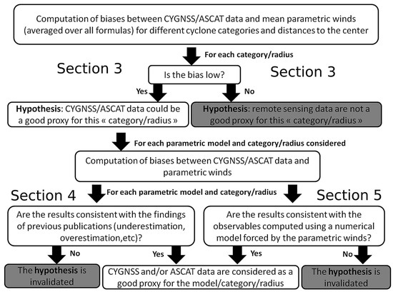
Figure 1.
Flowchart summarizing the key steps of this study.
- First, the biases between CYGNSS/ASCAT data and wind speeds inferred from the ensemble mean parametric winds (i.e., averaged over all formulas) are computed for different cyclone categories and distances to the center, to identify the cases for which CYGNSS and/or ASCAT could be good proxies for wind speeds. Due to the relatively large number of independent parametric formulations we consider (seven), individual errors are indeed expected to be trimmed down in such an ensemble mean.
- Second, based on assumptions about CYGNSS/ASCAT data, the biases of individual parametric models are computed to check whether our hypotheses enable reproduction of the findings of previous studies in terms of performance for wind gradient profiles.
- Third, we investigate whether our assumptions about CYGNSS/ASCAT data allow for identification of relevant parametric models for a specific case study: The category 5 hurricane Maria.
3. Comparison of CYGNSS and ASCAT Data
To get a preliminary idea of the usefulness of CYGNSS and ASCAT data as a proxy for surface wind speed, we compute the biases between these data and the mean (i.e., averaged over all empirical models) parametric winds for different cyclone categories and distances to the center (Figure 2). Computations are performed only when more than 30 data points are available for a given intensity/distance class. In practice, the comparison is possible in almost all cases, as hundreds to thousands of space-borne observations are available for each class. Parametric models are constrained by all the information provided by the NHC in the advisories to ensure that they give the best approximation possible of real winds. In classes for which the biases are large, remote sensing data are not consistent with the mean parametric winds. We choose not to investigate these cases further in the following sections, even if there is no evidence that the discrepancy is due to remote sensing errors rather than parametric models. On the contrary, small biases (in absolute terms) suggest that remote sensing data and parametric winds are consistent, so that they both give satisfactory results a priori. In the following, we will make the assumption that these CYGNSS/ASCAT data are indeed good proxies, and will also check whether or not this leads to consistent results.
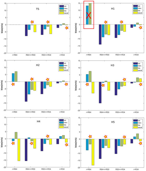
Figure 2.
Bias between the remote sensing data and the parametric winds averaged over all empirical models. Negative (resp. positive) values indicate that remote sensing data display lower (resp. higher) wind speeds compared to the mean parametric winds. Different categories of distance to the cyclone center (r) and cyclone intensities are considered. TS stands for tropical storms, H1, H2, H3, H4, and H5 to the Saffir-Simpson hurricane category (Cat 1, 2, 3, 4, and 5, respectively). R34, R50, and R64 are the radii for the 34-kt, 50-kt, and 64-kt winds. ws, nbrc, and les are three different CYGNSS products (see Section 2). The stars indicate which product has been selected as proxy for wind speeds in Section 4 and Section 5. The red box/cross shows the intensity/category class for which CYGNSS/ASCAT data are not expected to give adequate information about wind speeds.
Regarding ASCAT data, Figure 2 shows that the bias is low (less than about 2 m/s–3 m/s in absolute value) for wider radii than R34, but becomes increasingly negative with larger wind speeds, up to almost −20 m/s for category 5 cyclones and smaller radii than R64. These results suggest that ASCAT data are a good proxy for wind speeds lower than 34-kt, but that they underestimate extreme winds. This conclusion is consistent with previous published papers [48] based on methodologies and datasets different from ours.
The “wind speed” (ws) product is found to give systematically more negative biases than ASCAT, and thus probably often underestimates the velocities (Figure 2). However, the absolute value of bias remains relatively low for wider radii than R34, which suggests that this product might still be a good proxy for moderate and (potentially even more) low wind speeds. As this product was obtained for fully developed seas and not for cyclones, these results were also expected.
The LES and NBRCS products generally display lower biases for smaller radii than 50-kt, and are thus expected to outperform the other wind speed estimations close to the center of cyclones. Again, this finding is not surprising since these products have been derived using young seas/limited-fetch GMFs that are expected to be more suitable in strong cyclonic wind regions. It is not clear here whether one of these two products yields better results compared to the other, since they show similar biases of a few meters per second. It must be noted, however, that none of them is expected to perform well for smaller radii than R64 and category 1 storms, since the bias reaches very large values (10 m/s to 15 m/s). One plausible explanation is that the resolution of CYGNSS (25 km) is too low to capture the surface wind speeds in this range of radii for weak cyclones, for which the distance between the eyewall and the 64-kt wind radius is relatively small. Indeed, wind speeds vary quickly as a function of distance to the center in these regions. This issue is presumably less severe for stronger cyclones, because of their larger extent of hurricane-force winds (Table 1). It should also be recalled that close to the cyclone center, errors on NHC data may be sufficient to significantly reduce the accuracy of parametric wind speeds. This issue might be part of the reason why results are not satisfactory for smaller radii than R64 in the case of category 1 storms.
The results displayed in Figure 2 are used to make assumptions about the best proxy for wind speeds, depending on the considered radius and cyclone intensity. In the following sections, we will assume in particular that:
- ASCAT performs well for r > R34;
- ASCAT also performs well for R34 < r < R50 and category 3/5 cyclones (this product shows the lowest biases in these cases);
- none of the space-borne products tested here are reliable for smaller radii than R64 in the case of category 1 cyclones. We will not investigate these conditions in the next sections; and
4. Performance of Parametric Wind Models
Using the assumptions made in the previous section, we compute the bias in the various parametric models as a function of storm intensity, distance to the cyclone center, and calibration method (using only radii at 34-kt, only radii at 64-kt, and all radius information). The results are shown in Figure 3 and Figure 4. Blue colors correspond here to small biases (in absolute value), and thus suggest that the parametric model should work well for the intensity/distance class considered. Conversely, red colors suggest that the model will perform poorly.
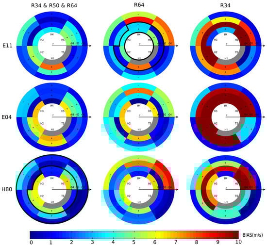
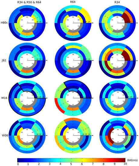
Figure 3.
Diagrams displaying the bias between various parametric models and the surface wind speeds estimated by CYGNSS/ASCAT data for all the events considered here, as a function of storm intensity and distance to the cyclone center, as well as calibration method (using all radius information, or only radii at 64-kt and 34-kt, for the left, middle and right panels, respectively). The color bar shows the absolute bias. The values are displayed for each category/distance cell. The black contours indicate the category/distance classes for which we consider E11 or H80 to build the E11H80 model in Section 5.
First of all, it appears that the bias is significantly reduced in almost all cases when constraining the parametric models by R64, R50, and R34. This suggests that not only the “mean” parametric wind values computed in Section 3 are consistent with the CYGNSS/ASCAT data: Almost all of the parametric models, taken individually, are also consistent, as long as they are constrained by the observations (i.e., the 64-kt, 50-kt, and 34-kt wind radii given by the NHC). This finding further validates the assumptions made in Section 3. One notable exception arises for radii between R64 and R50 for category 1 cyclones, for which the biases amount to 5 m/s or more in absolute value for most gradient wind profiles, even when constraining the wind fields with all the wind radius information. This suggests that the remote sensing data considered here as a proxy for wind speeds may be less accurate in this particular case. Referring back to Figure 2, CYGNSS products are seen to give negative biases similar to ASCAT for this radius/intensity class. Since ASCAT is expected to underestimate wind speeds for values larger than about 17 m/s [48], CYGNSS data can also be expected to do so in this case.
The strengths and weaknesses of each parametric formula can be investigated using the results shown in Figure 3 and Figure 4. For example:
- The inner region solution of Emanuel and Rotunno [36], E11, gives relatively small biases (hence, good results) close to the storm center, especially for intense and well defined cyclones. It is also found to underestimate wind speeds far from the center when constrained only by R64, as found in Lin and Chavas [17]. E04 performs better for the outer region, but poorly near the center. E11 and E04 can thus be merged to develop a complete TC radial wind structure as proposed by Chavas et al. [49];
- when solely constrained by radii close to the cyclone center (here R64), the Holland profile (H80) underestimates the winds in the outer region, as noted by Willoughby and Rahn [34]. This can also lead to broad wind maxima, and thus wind overestimations several dozens of kilometers from the center for strong cyclones, as can be seen also in Figure 3.
- J92 gives significantly higher wind speeds far from the center compared to most of the other parametric formulas, when constrained by R64 only. This is consistent with the findings of Lin and Chavas [17]. Our results suggest, however, that these wind speeds are generally not overestimated, and might better represent the wind decay as a function of the radius compared to other formulas;
- the results are generally much better when considering a family of profiles with two characteristic lengths, as proposed by Willoughby et al. [38]. For example, as stated above, the performance of the Holland model, H80, is significantly improved when both radii at 34-kt and 64-kt are prescribed; and
- models, such as W06 or M16 (which decay exponentially or as a power-law outside the eye), perform well in the outer region when the 34-kt radii are prescribed properly, which is consistent with the findings of Willoughby et al. [38] and Murty et al. [37].
The consistency of these results with the findings of past studies further suggests that the CYGNSS and ASCAT products are relatively good proxies for high and moderate surface wind speeds, respectively. The only exceptions are regions close to the eyewall, for which the spatial resolution is too low to capture the strong wind speed gradients (and where errors on NHC data may reduce the accuracy of wind speeds estimated using parametric models).
To further build confidence in our results, we perform numerical hindcasts of hurricane Maria (2017) in the following section (Section 5), and compare computed significant wave heights with real in-situ data. The aim is to investigate the potential of the results presented in Figure 3 and Figure 4 to objectively identify suitable parametric models.
5. Comparison with In-Situ Oceanic Data
Hurricane Maria was the deadliest storm of the 2017 Atlantic season. Recorded as a category 5 event, it caused catastrophic damage in Dominica and Puerto Rico, as well as widespread flooding and crop destructions in Guadeloupe. We test here the ability of the results presented in Figure 3 and Figure 4 to identify parametric models able to satisfactorily represent the temporal evolution of the wind pattern that took place during Maria. To do so, we compared the significant wave heights observed at buoys in the Lesser Antilles with those computed using a wave-current coupled model forced by a sub-set of the various parametric winds considered in the previous sections. The model is based on the code, SCHISM-WWM [50]. The computational domain is represented in Figure 5. Resolution spans from 10 km far from the region of interest (where the bathymetry is derived from GEBCO), up to about 100 m in Guadeloupe and Martinique, where we have the best bathymetric data (ship-based soundings from the SHOM, the French Naval Hydrographic and Oceanographic Department). The model is forced by:
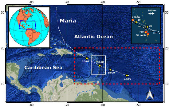
Figure 5.
Study area. The computational domain is depicted with the dashed red contour. The dashed white line represents the track of hurricane Maria. The location of the buoys used for comparison is given in the upper-right corner box. H3, H4, and H5 represent the Saffir-Simpson category of hurricane Maria along its trajectory.
- Astronomic tidal potential over the whole domain (12 constituents);
- 26 tidal harmonic constituents at the open boundaries, provided by the global FES2012 model [51];
- parametric pressure fields [33]; and
- parametric winds blended with CFSR (Climate Forecast System Reanalysis [52]) wind data. The parametric winds are prescribed for smaller radii than R34, whereas CFSR data are imposed for r > 1.5 R34. In between, a smooth transition is ensured using a weighing coefficient, which varies linearly with radius r.
We considered here six parametric models:
- E11 and H80, constrained using the 64-kt wind radii only (E11(R64) and H80(R64) in Figure 6);
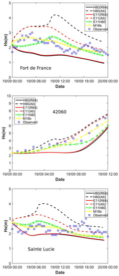 Figure 6. Significant wave height time series for different parametric models. “R64” denotes a model constrained only by the 64-kt wind radius. “ALL” indicates a model constrained with all the available information (34-kt, 50-kt, and 64-kt wind radii). E11H80 corresponds to a blend of the model E11 (for the inner core region) and H80 (for the outer region). M16b is the result of a blend between wind speeds obtained from M16 constrained by R64 only and with all wind radii information. Results for Fort-de-France, 42060, and the Sainte-Lucie station are displayed in the upper, middle, and lower panels, respectively.
 - E11 and H80, constrained using all the wind radii information (E11(All) and H80(All) in Figure 6);
- E11H80, for which we choose to blend the wind speeds inferred from E11 for the inner core region with those given by H80 for the outer region (see the black contours in Figure 3); and
- M16b, a blend between wind speeds obtained from M16 constrained by R64 only and with all wind radii information (see black contours in Figure 4).
E11H80 and M16b were chosen to test whether the results presented in Figure 3 and Figure 4 could be of benefit to build a relevant parametric model for the cyclone considered, using a combination of models that is expected to reduce the biases. We strongly emphasize the fact that the new models tested here are provided only as examples. They should in no way be considered as the “best” possible option. Better results can certainly be obtained with other wind gradient profiles. As an example, J92 also generally displays low biases, and could be a good candidate in a number of cases.
The reader is referred to Zhang et al. [50] and Krien et al. [9] for greater details about the model and the numerical strategy. Here, we compare the significant wave heights (Hs) computed by the model with Hs recorded by three buoys located in the Lesser Antilles (Figure 5): Fort de France (FdF) and Sainte Lucie, owned by Météo France, as well as 42060, maintained by the National Data Buoy Center (NDBC). The latter went adrift during the peak of Maria, hence the decrease in Hs was unfortunately not captured.
Results (Table3, Figure 6) show that:
- H80 and E11 constrained only by the 64-kt wind radius (R64) give the worst results, with Hs generally significantly underestimated, and NRMS ranging between 20% and 50% (Table 3). This is consistent with the results of Figure 3 and Figure 4, which show large negative biases for H80 and E11 in the case of category 4–5 cyclones and wider radii than R64;
Table 3. Bias, root mean square error (RMS), and RMS normalized by the mean observed values (NRMS) obtained when comparing numerical simulations with in-situ significant wave heights.
- constraining all the 34-kt, 50-kt, and 64-kt wind radii (All) results in better performance for E11, with reduced bias and NRMS (15% to 22% approximately), although significant wave heights are now overestimated. This is again consistent with the findings of Figure 3, which shows a positive bias at all radii for category 4 and 5 events;
- H80 constrained by all wind-radii information strongly overestimates Hs when Maria is closest to the storm. This is also consistent with the results of Figure 3 (and the findings of Willoughby and Rahn [34]), which show that H80 tends to overestimate wind speeds close to the center of strong (category 4–5) cyclones. The prediction is better when Maria moves further away, which is also expected and
- the best results are obtained for E11H80 and M16b, the two parametric models built to minimize the biases. NRMS values of the order of 9%–20% are obtained for significant wave heights, which is a good score considering the cyclone asymmetry due to the complexity of the area, characterized by a number of mountainous islands separated by just a few dozen kilometers.
These results, obtained with observed and completely independent data, support our assumption that the ASCAT and CYGNSS products are relatively good proxies for moderate and strong surface wind speeds, respectively, with the exception of the region close to the core for which higher spatial resolution is needed.
6. Conclusions
Taking advantage of an extremely active 2017 hurricane season in the tropical Atlantic Ocean and the Eastern Pacific, we investigated the feasibility of using the recent satellite remote sensing CYGNSS and ASCAT data to identify the strengths and weaknesses of several parametric wind models used for storm surge hazard assessment and the prediction of cyclonic waves.
Under the assumption that ASCAT and CYGNSS data can be considered as good proxies for surface wind speeds in the outer and inner regions, respectively (with an exception in the core of cyclones), we were able to confirm the findings of a number of previous studies (e.g., Willoughby et al. [38], Lin and Chavas [17], or Chavas et al. [49]) regarding biases present in several parametric models. Using a wave-current coupled numerical model, we also showed that this assumption is reasonable enough to be used to identify suitable parametric models for a specific case study.
We emphatically note that our aim here is not to encourage using or discarding a specific parametric model, nor to propose a new one. If we wanted to do that, we should have tested all published models. Such a comprehensive assessment is well beyond the scope of the current work. Besides, the models considered here have been tested with a unique combination of parameters (e.g., SWRF) and approaches to synthesize the wind field. It would be premature to draw definitive conclusions. In addition, it should be kept in mind that there are also errors in remote sensing data, so differences of 2 m/s–3 m/s in bias are probably not always significant.
The main finding of this paper is the following: Satellite remote sensing is now mature enough to provide relevant information about the structure of wind fields in cyclones, and can be used to assess the performance of parametric cyclonic wind models. Further work is yet needed to retrieve the detailed structure of TCs close to the eyewall. We focused here mainly on CYGNSS and ASCAT, but there is little doubt that other types of data may also be valuable. Remote sensing has now become a powerful tool that should be used to validate or improve existing parametric approaches, in order to conduct better wind, wave, and surge analyses for TCs.
It is noteworthy to conclude by mentioning that even with the models tested here for Maria (see Section 5), the NRMS remains significant (about 9%–20%). This might be attributed (at least partially) to the fact that the temporal resolution of the available track data (six hours) is not yet sufficient to allow parametric models to capture the short-term variations of track, translation speed, or wind asymmetry. This highlights the need for even higher temporal sampling of data (location of the cyclone center, maximum wind speed, wind radii, etc.), and for greater efforts to improve the efficiency of numerical atmospheric models.
Author Contributions
Y.K. conceived the idea and wrote most of the paper; G.A., R.C. and J.K. contributed to the development of the analysis tools; G.A., A.B. and A.K.M.S.I. arranged the figures and corrected a number of errors in the first version of the manuscript. C.R. wrote the description part on remote sensing data. D.B., P.P. and N.Z. prepared the project C3AF which funded about 66% of the work presented here. F.D., L.T. and A.K.M.S.I. played a major role for obtaining the IRD grant (about one third of total fundings). The manuscript also greatly benefited from their proofreading and suggestions.
Funding
This research was funded by the ERDF/C3AF project (grant number: CR/16-115) and the ANR/TIREX (ANR-18-OURA-0002-05). The main author also benefited from a grant by the IRD (Institut de Recherche pour le Développement).
Acknowledgments
Our warm thanks to the teams working on CYGNSS and ASCAT for their efforts, and to make the data available. ASCAT and CYGNSS data were provided here by the KNMI and PODAAC data center respectively. Data at Fort-de-France and Sainte-Lucie were made available by the CEREMA (CANDHIS database).The significant wave heights at station 42060 were provided by NDBC.
Conflicts of Interest
The authors declare no conflict of interest.
References
- Vickery, P.J.; Masters, F.J.; Powell, M.D.; Wadhera, D. Hurricane hazard modeling: The past, present, and future. J. Wind Eng. Ind. Aerodyn. 2009, 97, 392–405. [Google Scholar] [CrossRef]
- Lin, N.; Smith, J.A.; Villarini, G.; Marchok, T.P.; Baeck, M.L. Modeling extreme rainfall, winds, and surge from Hurricane Isabel (2003). Weather Forecast. 2010, 25, 1342–1361. [Google Scholar] [CrossRef]
- Hsiao, L.F.; Chen, D.S.; Kuo, Y.H.; Guo, Y.R.; Yeh, T.C.; Hong, J.S.; Fong, C.T.; Lee, C.S. Application of WRF 3DVAR to operational typhoon prediction in Taiwan: Impact of outer loop and partial cycling approaches. Weather Forecast. 2012, 27, 1249–1263. [Google Scholar] [CrossRef]
- Powers, J.; Klemp, J.; Skamarock, W.; Davis, C.; Dudhia, J.; Gill, D.; Coen, J.; Gochis, D.; Ahmadov, R.; Peckham, S.; et al. The weather research and forecasting (WRF) model: Overview, system efforts, and future directions. Bull. Am. Meteorol. Soc. 2017. [Google Scholar] [CrossRef]
- Lakshmi, D.; Murty, P.L.N.; Bhaskaran, P.K.; Sahoo, B.; Srinivasa Kumar, T.; Shenoi, S.S.C.; Srikanth, A.S. Performance of WRF-ARW winds on computed storm surge using hydrodynamic model for Phailin and Hudhud cyclones. Ocean Eng. 2017, 131, 135–148. [Google Scholar] [CrossRef]
- Mattocks, C.; Forbes, C. A real-time, event-triggered storm surge forecasting system for the state of North Carolina. Ocean Model. 2008, 25, 95–119. [Google Scholar] [CrossRef]
- Lin, N.; Emanuel, K.A. Grey swan tropical cyclones. Nat. Clim. Chang. 2016, 6, 106–111. [Google Scholar] [CrossRef]
- Orton, P.M.; Hall, T.M.; Talke, S.A.; Blumberg, A.F.; Georgas, N.; Vinogradov, S. A validated tropical-extratropical flood hazard assessment for New York harbor. J. Geophys. Res. Oceans 2016, 121, 8904–8929. [Google Scholar] [CrossRef]
- Krien, Y.; Testut, L.; Durand, F.; Mayet, C.; Islam, A.K.M.S.; Tazkia, A.R.; Becker, M.; Calmant, S.; Papa, F.; Ballu, V.; et al. Towards improved storm surge models in the northern Bay of Bengal. Cont. Shelf Res. 2017, 135, 58–73. [Google Scholar] [CrossRef]
- Shao, Z.; Liang, B.; Li, H.; Wu, G.; Wu, Z. Blended wind fields for wave modeling of tropical cyclones in the South China Sea and East China Sea. Appl. Ocean Res. 2018, 71, 20–33. [Google Scholar] [CrossRef]
- Feng, X.; Li, M.; Yin, B.; Yang, D.; Yang, H. Study of storm surge trends in typhoon-prone coastal areas based on observations and surge-wave coupled simulations. Int. J. Appl. Earth Obs. Geoinf. 2018. [Google Scholar] [CrossRef]
- Tan, C.; Fang, W. Mapping the Wind Hazard of Global Tropical Cyclones with Parametric Wind Field Models by Considering the Effect of Local Factors. Int. J. Disaster Risk Sci. 2018. [Google Scholar] [CrossRef]
- Niedoroda, A.W.; Resio, D.T.; Toro, G.R.; Divoky, D.; Das, H.S.; Reed, C.W. Analysis of the coastal Mississippi storm surge hazard. Ocean Eng. 2010, 37, 82–90. [Google Scholar] [CrossRef]
- Haigh, I.D.; MacPherson, L.R.; Mason, M.S.; Wijeratne, E.M.S.; Pattiaratchi, C.B.; Crompton, R.P.; George, S. Estimating present day extreme water level exceedance probabilities around the coastline of Australia: Tropical cyclone-induced storm surges. Clim. Dyn. 2014, 42, 139–157. [Google Scholar] [CrossRef]
- Krien, Y.; Dudon, B.; Roger, J.; Zahibo, N. Probabilistic hurricane-induced storm surge hazard assessment in Guadeloupe, Lesser Antilles. Nat. Hazards Earth Syst. Sci. 2015, 15, 1711–1720. [Google Scholar] [CrossRef]
- Krien, Y.; Dudon, B.; Roger, J.; Arnaud, G.; Zahibo, N. Assessing storm surge hazard and impact of sea level rise in Lesser Antilles-Case study of Martinique. Nat. Hazards Earth Syst. Sci. 2017, 17, 1559–1571. [Google Scholar] [CrossRef]
- Lin, N.; Chavas, D. On hurricane parametric wind and applications in storm surge modeling. J. Geophys. Res. 2012, 117, D09120. [Google Scholar] [CrossRef]
- Olfateh, M.; Callaghan, D.P.; Nielsen, P.; Baldock, T.E. Tropical cyclone wind field asymmetry—Development and evaluation of a new parametric model. J. Geophys. Res. Oceans 2017, 122, 458–469. [Google Scholar] [CrossRef]
- Knaff, J.A.; Longmore, S.P.; DeMaria, R.T.; Molenar, D.A. Improved Tropical-Cyclone Flight-Level Wind Estimates Using Routine Infrared Satellite Reconnaissance. J. Appl. Meteorol. Clim. 2015, 54, 463–478. [Google Scholar] [CrossRef]
- Dolling, K.; Ritchie, E.; Tyo, J. The Use of the Deviation Angle Variance Technique on Geostationary Satellite Imagery to Estimate Tropical Cyclone Size Parameters. Weather Forecast. 2016, 31, 1625–1642. [Google Scholar] [CrossRef]
- Mueller, K.J.; DeMaria, M.; Knaff, J.A.; Kossin, J.P.; VonderHaar, T.H. Objective estimation of tropical cyclone wind structure from infrared satellite data. Weather Forecast. 2006, 21, 990–1005. [Google Scholar] [CrossRef]
- Figa-Saldana, J.; Wilson, J.J.W.; Attema, E.; Gelsthorpe, R.; Drinkwater, M.R.; Stoffelen, A. The advanced scatterometer (ASCAT) on the meteorological operational (MetOp) platform: A follow on for European wind scatterometers. Can. J. Remote Sens. 2002, 28, 404–412. [Google Scholar] [CrossRef]
- Madsen, N.M.; Long, D.G. Calibration and Validation of the RapidScat Scatterometer Using Tropical Rainforests. IEEE Trans. Geosci. Remote Sens. 2016, 54, 2846–2854. [Google Scholar] [CrossRef]
- Meissner, T.; Wentz, F.J. Wind vector retrievals under rain with passive satellite microwave radiometers. IEEE Trans. Geosci. Remote Sens. 2009, 47, 3065–3083. [Google Scholar] [CrossRef]
- El-Nimri, S.F.; Lindwood Jones, W.; Uhlhorn, E.; Ruf, C.; Johnson, J.; Black, P. An improved C-band ocean surface emissivity model at hurricane-force wind speeds over a wide range of Earth incidence angles. IEEE Geosci. Remote Sens. Lett. 2010, 7, 641–645. [Google Scholar] [CrossRef]
- Reul, N.; Tenerelli, J.; Chapron, B.; Vandemark, D.; Quilfen, Y.; Kerr, Y. SMOS satellite L-band radiometer: A new capability for ocean surface remote sensing in hurricanes. J. Geophys. Res. 2012, 117, C02006. [Google Scholar] [CrossRef]
- Reul, N.; Chapron, B.; Zabolotskikh, E.; Donion, C.; Mouche, A.A.; Tenerelli, J.; Collard, F.; Piolle, J.F.; Fore, A.; Yueh, S.; et al. A new generation of tropical cyclone size measurements from space. Bull. Am. Meteorol. Soc. 2017, 98, 2367–2385. [Google Scholar] [CrossRef]
- Zabolotskikh, E.; Mitnik, L.M.; Reul, N.; Chapron, B. New Possibilities for Geophysical Parameter Retrievals Opened by GCOM-W1 AMSR2. IEEE J. Sel. Top. Appl. Earth Obs. Remote Sens. 2015, PP, 1–14. [Google Scholar] [CrossRef]
- Fore, A.G.; Yueh, S.H.; Tang, W.; Stiles, B.; Hayashi, A.K. Combined Active/Passive Retrievals of Ocean Vector Wind and Sea Surface Salinity with SMAP. IEEE Trans. Geosci. Remote Sens. 2016, 54, 7396–7404. [Google Scholar] [CrossRef]
- Foti, G.; Gommenginger, C.; Jales, P.; Unwin, M.; Shaw, A.; Robertson, C.; Rosell, J. Spaceborne GNSS reflectometry for ocean winds: First results from the UK TechDemoSat-1 mission. Geophys. Res. Lett. 2015, 42, 5435–5441. [Google Scholar] [CrossRef]
- Ruf, C.S.; Atlas, R.; Chang, P.S.; Clarizia, M.P.; Garrison, J.L.; Gleason, S.; Katzberg, S.J.; Jelenak, Z.; Johnson, J.T.; Majumdar, S.J.; et al. New Ocean Winds Satellite Mission to Probe Hurricanes and Tropical Convection. Bull. Am. Meteorol. Soc. 2016, 97, 385–395. [Google Scholar] [CrossRef]
- Morris, M.; Ruf, C. Determining Tropical Cyclone Surface Wind Speed Structure and Intensity with the CYGNSS Satellite Constellation. J. Appl. Meteorol. Clim. 2017. [Google Scholar] [CrossRef]
- Holland, G. An Analytic Model of the Wind and Pressure Profiles in Hurricanes. Mon. Weather Rev. 1980, 108, 1212–1218. [Google Scholar] [CrossRef]
- Willoughby, H.E.; Rahn, M.E. Parametric representation of the primary hurricane vortex. Part I: Observations and evaluation of the Holland (1980) model. Mon. Weather Rev. 2004, 132, 3033–3048. [Google Scholar] [CrossRef]
- Jelesnianski, C.P.; Taylor, A.D. A Preliminary View of Storm Surges before and after Storm Modifications; NOAA Technical Memorandum, ERL WMPO-3; Environmental Research Laboratories, Weather Modification Program Office: Boulder, CO, USA, 1973; p. 33. [Google Scholar]
- Emanuel, K.; Rotunno, R. Self-stratification of tropical cyclone outflow, Part I: Implications for storm structure. J. Atmos. Sci. 2011, 68, 2236–2249. [Google Scholar] [CrossRef]
- Murty, P.L.N.; Bhaskaran, P.K.; Gayathri, R.; Sahoo, B.; Srinivasa Kumar, T.; SubbaReddy, B. Numerical study of coastal hydrodynamics using a coupled model for Hudhud cyclone in the Bay of Bengal. Estuar.Coast. Shelf Sci. 2016, 183, 13–27. [Google Scholar] [CrossRef]
- Willoughby, H.E.; Rahn, M.E.; Darling, R.W.R. Parametric representation of the primary hurricane vortex. Part II: A new family of sectionally continuous profiles. Mon. Weather Rev. 2006, 134, 1102–1120. [Google Scholar] [CrossRef]
- Powell, M.D.; Vickery, P.J.; Reinhold, T.A. Reduced drag coefficient for high wind speeds in tropical cyclones. Nature 2003, 422, 279–283. [Google Scholar] [CrossRef] [PubMed]
- Uhlhorn, E.W.; Black, P.G.; Franklin, J.L.; Goodberlet, M.A.; Carswell, J.R.; Goldstein, A.S. Hurricane surface wind measurements from an operational stepped frequency microwave radiometer. Mon. Weather. Rev. 2007, 135, 3070–3085. [Google Scholar] [CrossRef]
- Ruf, C.S.; Gleason, S.; McKague, D.S. Assessment of CYGNSS Wind Speed Retrieval Uncertainty. IEEE J. Sel. Top. Appl. Earth Obs. Remote Sens. 2018, PP, 1–11. [Google Scholar] [CrossRef]
- Saïd, F.; Katzberg, S.J.; Soisuvarn, S. Retrieving Hurricane Maximum Winds Using Simulated CYGNSS Power-Versus-Delay Waveforms. IEEE J. Sel. Top. Appl. Earth Obs. Remote Sens. 2017, 10, 3799–3809. [Google Scholar] [CrossRef]
- ASCAT Wind Product User Manual, KNMI, De Bit, The Netherlands. 2013. Available online: http://projects.knmi.nl/ scatterometer/publications/pdf/ASCAT_Product_Manual.pdf. (accessed on 1 October 2018).
- Verhoef, A.; Portabella, M.; Stoffelen, A. High-resolution ASCAT scatterometer winds near the coast. IEEE Trans. Geosci. Remote Sens. 2012, 50, 2481–2487. [Google Scholar] [CrossRef]
- Hu, K.; Chen, Q.; Kimball, S.K. Consistency in hurricane surface wind forecasting: An improved parametric model. Nat. Hazards 2012, 61, 1029–1050. [Google Scholar] [CrossRef]
- Emanuel, K. Tropical cyclone energetics and structure. In Atmospheric Turbulence and Mesoscale Meteorology; Fedorovich, E., Rotunno, R., Stevens, B., Eds.; Cambridge University Press: Cambridge, UK, 2004; pp. 165–192. [Google Scholar]
- Jelesnianski, C.P.; Chen, J.; Shaffer, W.A. SLOSH: Sea, Lake, and Overland Surges from Hurricanes; NOAA Technical Report NWS 48; NOAA AOML Library: Miami, FL, USA, 1992. [Google Scholar]
- Brennan, M.J.; Hennon, C.C.; Knabb, R.D. The Operational Use of QuikSCAT Ocean Surface Vector Winds at the National Hurricane Center. Weather Forecast. 2009, 24, 621–645. [Google Scholar] [CrossRef]
- Chavas, D.R.; Lin, N.; Emanuel, K. A model for the complete radial structure of the tropical cyclone wind field. Part I: Comparison with observed structure. J. Atmos. Sci. 2015, 72, 3647–3662. [Google Scholar] [CrossRef]
- Zhang, Y.; Ye, F.; Stanev, E.V.; Grashorn, S. Seamless cross-scale modeling with SCHISM. Ocean Model. 2016, 102, 64–81. [Google Scholar] [CrossRef]
- Carrère, L.; Lyard, F.; Cancet, M.; Guillot, A.; Roblou, L. FES2012: A new global tidal model taking advantage of nearly 20 years of altimetry. Paper presented at Proceedings of The Symposium 20 Years of Progress in Radar Altimetry, Venice-Lido, Italy, 24–29 September 2012. [Google Scholar]
- Saha, S.; Moorthi, S.; Wu, X.; Wang, J.; Nadiga, S.; Tripp, P.; Behringer, D.; Hou, Y.T.; Chuang, U.Y.; Iredell, M.; et al. NCEP Climate Forecast System Version 2(CFSv2) Monthly Products; Research Data Archive at the National Center for Atmospheric Research; Computational and Information Systems Laboratory: Boulder, CO, USA, 2012. [Google Scholar]


© 2018 by the authors. Licensee MDPI, Basel, Switzerland. This article is an open access article distributed under the terms and conditions of the Creative Commons Attribution (CC BY) license (http://creativecommons.org/licenses/by/4.0/).