Abstract
The downward-looking sparse linear array three-dimensional synthetic aperture radar (DLSLA 3D SAR) has attracted a great deal of attention, due to the ability to obtain three-dimensional (3D) images. However, if the velocity and the yaw rate of the platform are not measured with enough accuracy, the azimuth signal cannot be compressed and then the 3D image of the scene cannot be obtained. In this paper, we propose a method for platform motion parameter estimation, and downward-looking 3D SAR imaging. A DLSLA 3D SAR imaging model including yaw rate was established. We then calculated the Doppler frequency modulation, which is related to the cross-track coordinates rather than the azimuth coordinates. Thus, the cross-track signal reconstruction was realized. Furthermore, based on the minimum entropy criterion (MEC), the velocity and yaw rate of the platform were accurately estimated, and the azimuth signal compression was also realized. Moreover, a deformation correction procedure was designed to improve the quality of the image. Simulation results were given to demonstrate the validity of the proposed method.
1. Introduction
Three-dimensional synthetic aperture radar (3D SAR) imaging can obtain 3D images of targets, and obtain more abundant target information than traditional SAR imaging, which often suffers from shading and layover effects [1,2,3]. Compared with other 3D SAR techniques, e.g., SAR tomography [4,5], which is a multi-baseline extension and employs many passes over the same area, downward-looking sparse linear array 3D SAR (DLSLA 3D SAR) can obtain the 3D image by single voyage and works in a more flexible mode [6,7]. The 3D resolution is acquired by pulse compression with wideband chirp signal, along-track aperture synthesis with flying platform movement, and cross-track aperture synthesis with physical sparse linear arrays [8,9,10]. In a practical system, array distribution is usually non-uniform and sparse due to some inevitable factors, e.g., installation restriction, wing vibration, etc. [11,12].
Existing DLSLA 3D SAR researchers have been focusing on three main aspects: Imaging methods, array optimization, and improving the cross-track resolution. Uniform linear array imaging algorithms are usually based on the beam-forming theory and multiple signal classification (MUSIC) algorithm to realize 3D imaging [13,14]. Sparse array methods exploit the sparsity of the 3D scene, and employ compressed sensing (CS) [15,16] and regularization methods [17] for DLSLA 3D SAR imaging [18,19]. Under the traditional CS framework, the continuous scene must be discretized. However, the coordinates to be estimated do not usually fall on discrete points, which may cause the off-grid effect [20,21]. To mitigate against the off-grid effect, continuous CS (CCS) based on atomic norm minimization (ANM) is applied to DLSLA 3D SAR [22]. A multilayer first-order approximation model is also proposed in [23] to deal with this issue. On the other hand, for sparse array methods, designing the arrays to obtain better imaging effects is a key research topic. An array design method based on the spatial convolution principle is proposed in [24]. An array optimization method based on the minimum average mutual coherence of the observation matrix is proposed in [25]. A particular issue in DLSLA 3D SAR imaging is that the cross-track resolution is relatively low, because the length of the array is limited by the platform size. Thus, a large amount of research is focused on how to improve the cross-track resolution, e.g., the two dimensional smoothed L0 (2D SL0) algorithm [26], the Bayesian compressed sensing algorithm [27], etc.
However, the above articles do not consider signal processing under non-ideal conditions. In practical applications, the actual path of the platform usually deviates from its ideal path. A joint multi-channel auto-focusing technology is proposed in [28] to estimate motion error, but the performance of this method is degraded when the synthetic aperture time is short. A method based on wavenumber domain sub-block is proposed in [29] to compensate the yaw angle error, but this method requires the velocity and yaw angle to be known, which restricts its application. Moreover, the yaw angle will cause image deformation, another aspect that was not considered. Actually, there is a difference between traditional SAR and DLSLA 3D SAR in motion compensation. Conventional SAR usually works in a long-range imaging mode, which has the characteristics of long synthetic aperture and long synthetic aperture time. Therefore, it is necessary to compensate the motion error with the sub-aperture technique [30,31]. However, in DLSLA 3D SAR, the cross-track resolution depends on the wavelength of the transmitted signal, the length of the array, and the flying height of the platform. Due to the fact that the length of the array is limited by the platform size, the flying height of the platform cannot be too high if the cross-track resolution is to be within an acceptable level. When the flying height of the platform is limited, the corresponding synthetic aperture length will be relatively short, resulting in a very short synthetic aperture time, especially for fast moving platforms. Thus, it can be considered that platform motion is constant during the synthetic aperture time. As long as the motion parameters of the platform are obtained, they can be used to construct a compensation function to compensate for motion errors and realize 3D imaging of the scene.
Based on the above analysis, this paper considers the situation where there is a yaw rate when the platform flies, and that the velocity and yaw rate obtained by the airborne measuring equipment are inaccurate. We proposed the following solutions: First, an imaging model of DLSLA 3D SAR with yaw rate was established; and second, the Doppler frequency modulation was calculated from the modulated cross-track coordinates (rather than the modulated azimuth coordinates). As a result, cross-track signal processing was carried out to obtain the cross-track coordinates before azimuth signal processing. Based on the minimum entropy criterion (MEC), the velocity and yaw rate of the platform were estimated, and the azimuth signal compression was also realized. Moreover, a deformation correction procedure was designed to improve the quality of the image. Compared with the existing methods, the proposed method was able to estimate the platform motion parameters precisely and achieve better imaging results. Simulation results demonstrated the validity of the proposed method.
The remainder of this paper is organized as follows: The imaging model is established and the Doppler frequency modulation is analyzed in Section 2; in Section 3, cross-track signal reconstruction is discussed; parameter estimation and the azimuth compression based on MEC are described in Section 4; deformation correction is presented in Section 5; simulation experiments are carried out in Section 6; and some conclusions are drawn in Section 7.
2. DLSLA 3D SAR Imaging Model
The imaging geometry of airborne DLSLA 3D SAR is shown in Figure 1. In the downward-looking working mode, the beam illuminates the area below the platform. The platform flies at the altitude H with velocity v. The flight path (azimuth direction) is paralleled to the X-axis. The sparse linear array is obtained by random selection on a uniform linear array, which is mounted underneath the wings along the cross-track direction (Y-axis) and symmetrical about the Z-axis. The Z-axis denotes the height direction (range direction), which is also the line of sight of the radar. That is, the height resolution is dependent on the transmitted wideband chirp signal. The azimuth resolution is dependent on the synthesis aperture formed by the platform flying, and the cross-track resolution is dependent on the real aperture formed by the sparse linear array. Suppose the sequence vector of uniform linear array with spacing 2d is and the sparse linear array is obtained by random selection from a uniform linear array. The value of d can be set as half of the wavelength [32]. The hollow circle “” in the middle represents the transmitting array and the solid circles “” on both sides represent the receiving arrays. According to the equivalent phase centers (EPCs) principle [33,34], N arrays can obtain N EPCs. By random selection from a uniform linear array, the number P of sparse EPCs can be obtained with . The obtained sparse EPC sequence vector can be denoted as , with . Thus, the EPC is located at at slow time , where and . For the pth EPC, the ideal instantaneous distance from the array to the kth scatterer in the imaging scene is:
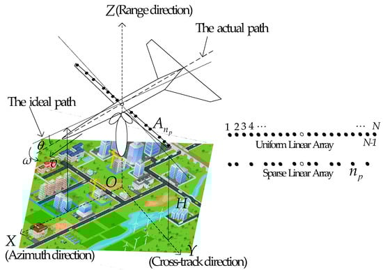
Figure 1.
DLSLA 3D SAR imaging geometry model.
Actually, due to the influence of air disturbance, the platform may deviate from its ideal path, which will affect the DLSLA 3D SAR imaging. Assume there is a yaw rate ω in the flight. The in Figure 1 denotes the intersection angle between the ideal and actual paths. The actual instantaneous distance from the EPC to the kth scatterer is:
where , , and .
Assuming the radar transmits a linear frequency modulation (LFM) signal with the center frequency fc. In the far field, the received data of the EPC can be expressed as:
where D is the imaging region, is the reflectance of the kth scatterer, is the fast time, is the electromagnetic wave speed, and is the chirp rate.
Errors caused by EPC can be compensated using the method in [19]. When the range compression is completed and the errors caused by EPC are compensated, the echo signal in the time domain after scene discretization can be expressed as:
Thus, the signal represented by Equation (4) can be seen as a series of two-dimensional signals with different heights. Then, the two-dimensional signal of azimuth and cross-track of the ith range (height) cell is:
where is the constant phase, represents the range value of the ith range cell, and L represents the number of scatterers in the ith range cell.
Assuming the yaw rate is ω, and the initial yaw angle is θ0. Then the instantaneous yaw angle is . The instantaneous Doppler frequency can be obtained as follows:
where is the wavelength. Furthermore, the Doppler frequency modulation can be obtained by the following expression:
Referring to the definitions of instantaneous Doppler and Doppler frequency modulations, the instantaneous frequency and frequency modulation of cross-track signal can be denoted as:
Equation (9) shows that is a constant, so the cross-track signal can be processed directly. According to Equations (6) and (8), the Doppler frequency center and the cross-track frequency center are:
Equations (10) and (11) indicate that the focused image is deformed. More specifically, the azimuth coordinate and cross-track coordinate are modulated. That is, after image focusing, deformation correction is required to improve the quality of the image.
Assuming that the plane is flying smoothly, the yaw rate ω is kept small and θ is changing slowly. From experience, typical values are , and [35,36]. Thus, the terms that contain factor can be ignored. Then, Equation (7) can be approximately expressed as:
Equation (12) indicates that the Doppler frequency modulation is space-variant, which is related not only to velocity and yaw rate, but also to the coordinates of the target.
Denote
then
then, Equations (11) and (12) can be further approximately expressed as:
According to Equations (9), (10), (17), and (18), the two-dimensional signal of azimuth and cross-track of the ith range cell can be constructed as:
where the first phase term represents the azimuth information and the second phase term represents the cross-track information. Equation (18) shows that the Doppler frequency modulation is related to the modulated cross-track coordinates and unrelated to the modulated azimuth coordinates. It also shows that the azimuth information is not contained in the second phase term of Equation (19), so the cross-track signal can be processed to obtain the modulated cross-track coordinates of scatterers before azimuth signal processing.
3. Cross-Track Signal Reconstruction with CS
For the azimuth and cross-track signals, each slow time sampling tm can be seen as a snapshot. According to Equation (19), the cross-track signal of a single snapshot can be expressed as:
where L denotes the total number at the ith range cell, , denotes the azimuthal phase corresponding to the slow time , and . After removing the independent quadratic phase terms, Equation (20) can be rewritten as:
Generally, in 3D SAR imaging, there are large amounts of non-target zones in the 3D scene. It means that the cross-track signal to be reconstructed is sparse. Thus, the cross-track signal can be processed with the CS method.
Firstly, the cross-track scene needed to be discretized. The cross-track imaging scene can be divided into Q equal intervals and the corresponding grid coordinates can be represented as , where , . is half the width of the region of interest, and the grid interval is . Then, the dictionary matrix of cross-track signal can be denoted as:
where , and .
Assuming , and , signal can be further expressed as:
where represents the noise. Equation (23) can be solved with the CS method in [23].
4. Minimum Entropy Criterion for Azimuth Compression
Image entropy closely relates to the quality of image focus. It is generally acknowledged that SAR images with a better focusing quality have smaller entropy.
According to Equation (18), the Doppler frequency modulation is related to the velocity, yaw rate, and modulated cross-track coordinates. The modulated cross-track coordinates were obtained in Section 3, so the velocity and yaw rate are the parameters to be estimated next. Meanwhile, in the same range and cross-track cells, targets located in different azimuth cells have the same Doppler frequency modulation.
After range compression and cross-track reconstruction, for scatterers in the ith range cell and lth cross-track cell, the azimuth signal can be denoted as:
where G is the number of scatterers in the ith range cell and lth cross-track cell.
According to the expression of Doppler frequency modulation, the compensation function can be constructed as:
where η is the phase compensation factor, which represents the Doppler frequency modulation; and represents the Doppler frequency, .
The phase compensation operation can be completed by matrix operation. Assuming decided by η is the signal after compensation, then can be denoted as:
where denotes the discrete Fourier transform (DFT) matrix with size M, denotes inverse discrete Fourier transform (IDFT) matrix with size M, represents the Hadamard product, , and . According to the image entropy definition, the image entropy of can be defined as:
where represents the mth element of vector , , represents the Euclidean norm operator. The image entropy can be used to evaluate the image focus quality, that is to say, when the entropy reaches minimum, the corresponding phase compensation factor η is the required value. The result can be obtained by solving the following optimization problem:
It is not easy to solve the above optimization problem directly. To simplify the optimization problem, a substitution function can be constructed to replace the objective function of Equation (28). The substitution function is designed as follows:
where is the uth iteration value, which is known in the uth iteration. Furthermore, the accurate phase compensation factor η can be obtained by an iterative algorithm, i.e., the problem of minimum entropy can be solved with the following iteration problem:
Through solving the above problem, the convergence value of the phase compensation factor η can be obtained. Then, the azimuth compression can be carried out with the compensation function . The flowchart is shown in Figure 2.
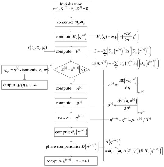
Figure 2.
The flow chart of MEC.
In Figure 2, is the velocity obtained by airborne measuring equipment. The concrete derive of and is shown in Appendix A. represents the step length, which is selected by the following searching method: Assuming the set of candidate values of step length is , each step length can obtain an image entropy value. Then, the step length corresponding to the minimum entropy can be taken as the required step length among these candidate values in this iteration.
5. Deformation Correction
After the above operation, a 3D image is obtained, albeit with the scatterers’ coordinates still modulated by the yaw angle. For a scatterer k located at , its coordinates obtained by the focused image can be denoted as , i.e., the azimuth and cross-track coordinates are modulated. The 3D image has been deformed and needs to be corrected.
It is noted that the starting time and the ending time of scatterer k can be obtained from the signal before azimuth compression.
Then from and velocity v, the theoretical starting time , and the theoretical ending time can be expressed as in Equations (31) and (32), respectively:
where is the synthetic aperture length. Therefore, the relationship between the azimuth coordinates before and after modulation can be expressed as:
or
When combining Equations (13), (14), with (33) or (34), there are three unknown parameters, namely ,
and the initial yaw angle . By solving this system of equations, the unknown parameters can be obtained. Thus, the accurate coordinates are obtained and the deformation correction is also completed.
The flow chart of the proposed method is shown in Figure 3.
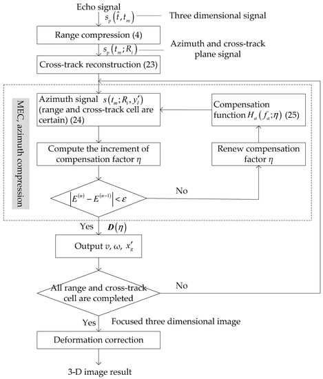
Figure 3.
The flow chart of the proposed method.
6. Experiments and Results
In this section, some experiments are presented to illustrate the performance of the proposed method.
6.1. DLSLA 3D SAR Imaging of Isolated Targets
In this subsection, isolated targets simulation is shown to verify the proposed method for DLSLA 3D SAR imaging. The parameters of simulation are listed in Table 1. The interval of linear array is d = 0.009 m. There were 20 isolated targets with the unit reflectivity in the Cartesian coordinates system, as shown in Figure 4.

Table 1.
Parameters of platform and antenna.
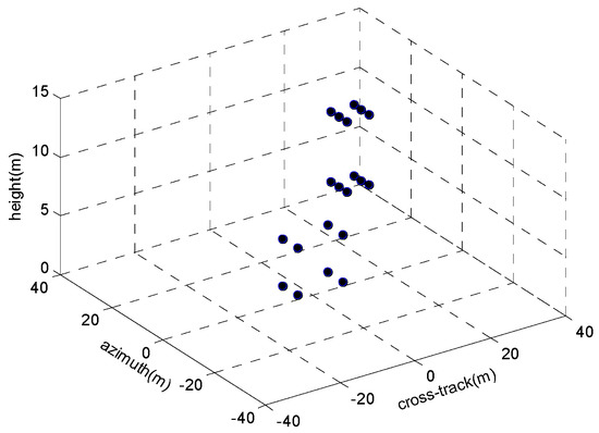
Figure 4.
3D isolated targets model.
In the simulation experiments, it was assumed that the velocity and the yaw rate obtained by the airborne measuring equipment were 62 m/s and 0 °/s, respectively. Noise was added to the signal after range compression, and the signal to noise ratio (SNR) was 5dB. The simulation results are shown in Figure 5. The imaging result after range compression and cross-track reconstruction with iterative shrinkage thresholding (IST) algorithm is shown in Figure 5a. The ratio of randomly selected array elements to the total linear uniform array elements was 0.875. Figure 5b shows the imaging results after azimuth compression from the Traditional Method (TM), with motion compensation function derived from parameters obtained by the airborne measuring equipment. It shows that the azimuth broadening exists, because these parameters obtained by the airborne measuring equipment were inaccurate. Figure 5c was obtained by autofocusing of the MapDrift (MD) method [24]. Compared to Figure 5b, the quality of Figure 5c was greatly improved. Figure 5d shows the imaging result obtained by the MEC before deformation correction. It shows that the azimuth signal was completely compressed, which demonstrated that the proposed MEC method can obtain the focused imaging result. Meanwhile, the estimation results of velocity and yaw rate were = 59.91 m/s and = 2.09 °/s, respectively. This meant that the proposed method can accurately estimate the parameter value and compensate for motion error.
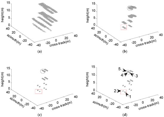
Figure 5.
Imaging result: (a) 3D imaging result after range compression and cross-track reconstruction; (b) 3D imaging result by traditional method; (c) 3D imaging result by MapDrift method; and (d) 3D imaging result by the proposed method.
To evaluate the azimuth imaging quality of the proposed method, the azimuth sectional images of the rectangular and ellipse areas of Figure 5 are shown in Figure 6a,b. It shows that the azimuth signal obtained by the TM had an obvious broadening phenomenon. The poor quality of the TM was due to parameter inaccuracies. The imaging result obtained by the MD method was better than that of TM. However, a prominent isolated target in each azimuth sectional image was necessary for satisfactory imaging results with the MD method. When the isolated targets in the scene were uniformly distributed, the estimation performance decreased, as shown in Figure 6b. The quality of the image obtained by the MEC was the best of the three methods. Figure 6 shows that the MEC can achieve azimuth signal compression and compensate for motion error. That is, the proposed method is valid.
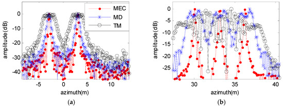
The 3dB width of the five targets with MD and MEC methods are shown in Table 2, where “improvement: Is defined as the ratio of the width of MD to the width of MEC”. Targets 1 and 2 correspond to targets in Figure 6a; and targets 3, 4, and 5 correspond to targets in Figure 6b. Table 2 shows that the performance of the MEC method was greatly improved.
Table 2.
The 3dB width of MD and MEC.
According to the analysis, the azimuth and cross-track coordinates obtained were modulated. The 2D projection image of Figure 5a onto azimuth and cross-track is shown in Figure 7a. The ending time of the echo signal is also shown in Figure 7a. The 2D projection image of Figure 5d onto azimuth and cross-track is shown in Figure 7b. It shows that the coordinates obtained were modulated, with region 1 more severe than that of region 2, because modulation increased with coordinates. Meanwhile, according to Figure 7b, the modulated azimuth coordinate was also obtained. Then, the theoretical echo signal ending time of was obtained. Finally, according to Equations (13), (14), and (45), the accurate coordinates were obtained and the initial yaw angle was obtained as 2.92°. Figure 7c shows the 2D projection result after deformation correction. It indicates that the azimuth coordinates have been corrected. However, due to the relatively poor cross-track resolution limited by the length of the antenna array, the correction effect of cross-track coordinates was not distinctive, so there is a deviation between the estimated values and the real values of cross-track coordinates.
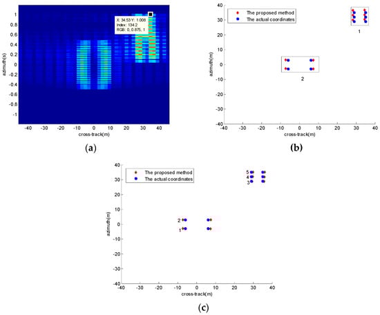
Figure 7.
2D projection onto azimuth and cross-track plane: (a) Before azimuth compression; (b) before deformation correction; and (c) after deformation correction.
Figure 8 shows the coordinates of target 3 (Figure 7c) before and after deformation correction. The azimuth and cross-track coordinates before and after deformation correction of the 5 targets are shown in Table 3. Take target 1 as an example, the definition of improvement in azimuth is that (distance to actual position before correction)/(distance to actual position after correction) = |(−2.81 − (−3))/(−2.91 − (−3))| = 2.11. Obviously, it means that the deformation correction was effective when the improvement value was greater than 1; the larger the improvement value, the more improvement of the imaging result accuracy. Table 3 shows that the improvements of azimuth coordinate were significant. Due to the low resolution, the improvements of cross-track were not obvious. In general, the deformation correction method is valid.
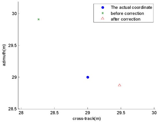
Figure 8.
The azimuth and cross-track coordinates before and after deformation correction of target 3.
Table 3.
The azimuth and cross-track coordinates before and after deformation correction.
During azimuth compression, the range cell and cross-track cell were determined. Figure 9 shows the corresponding image entropy convergence of an azimuth signal under different SNRs. In each iteration, the step length was determined by the searching method. The convergence threshold was set as .
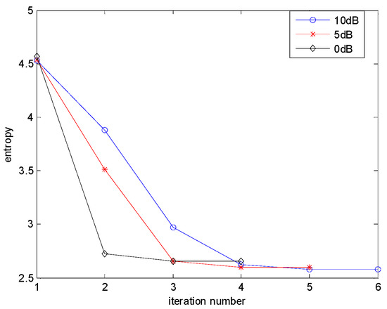
Figure 9.
Image entropy convergence curve.
6.2. DLSLA 3D SAR Imaging of Distributed Extended Targets
In this subsection, the DEM data of an airborne CSAR 2D image [37] were used to represent a distributed scene. The scene had an extent of in the Cartesian coordinates system with the radar system parameters listed in Table 1. The azimuth coordinates of scatterers were uniformly distributed in [−100 m, 100 m] with 1 m intervals. The cross-track coordinates of scatterers were also uniformly distributed in [−100 m, 100 m] with 1 m intervals. The ideal 3D distributed scene is shown in Figure 10a, and its 2D projection onto azimuth and cross-track plane is shown in Figure 10b. According to the system parameters, the cross-track Rayleigh resolution was 6.25 m. The SNR was chosen as 5 dB after range compression. The ratio of randomly selected array elements to the total linear uniform array elements was 0.875. The 3D reconstructed image by the proposed method shown in Figure 11a,b gives the corresponding image obtained by the traditional method. Here, the traditional method meant that using the parameter obtained by the airborne measuring equipment to carry out azimuth compression, where the velocity and the yaw rate were given as 62 m/s and 0 °/s, respectively. The imaging result by the traditional method clearly suffered from broadening phenomenon, and lost many image details. On the contrary, the proposed method obtained a good 3D image of the scene. Based on the minimum entropy method, on the other hand, the velocity and yaw rate were estimated as = 59.90 m/s and = 2.06 °/s, respectively. Further, the projection images onto the azimuth and cross-track plane by the two methods are illustrated in Figure 12a,b. It is seen that the coordinates of targets were affected by the deformation in both figures. Figure 13 shows the azimuth sectional image of a corresponding (range and cross-track cell) in Figure 12a,b. It is clear that TM (Figure 12b) suffered from the broadening phenomenon. However, because of the influence of range sidelobes, the azimuth sectional image of distributed targets (MEC, Figure 12a) was not as ideal as that of isolated targets (shown previously in Figure 6). By using the deformation correction method, the corrected result of Figure 12a is shown in Figure 14. The obtained initial yaw angle was 3.08°, which was very close to the real value. Comparing Figure 14 with Figure 10b, showed that the modulated coordinates in Figure 12a were corrected. In addition, the azimuth and cross-track coordinates before and after deformation correction of the 4 scatterers in Figure 10b are shown in Table 4. It can be found that the improvements of azimuth coordinate were significant.
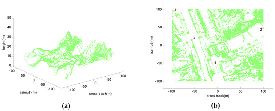
Figure 10.
The ideal scene: (a) The ideal 3D distributed scene; and (b) the 2D projection of ideal 3D scene onto azimuth and cross-track plane.
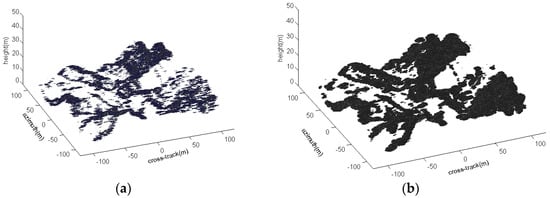
Figure 11.
3D imaging result of scene: (a) The proposed method; and (b) the traditional method.
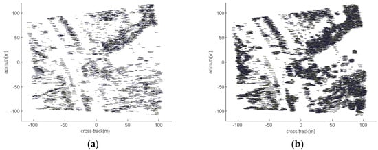
Figure 12.
2D projection onto azimuth and cross-track plane: (a) The proposed method; and (b) the traditional method.
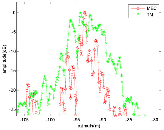
Figure 13.
The azimuth sectional image of MEC and TM methods.
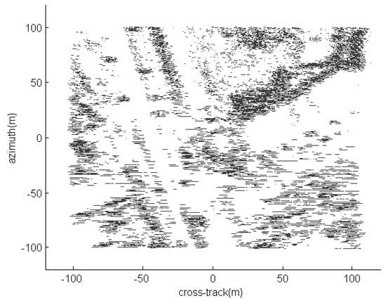
Figure 14.
2D projection onto azimuth and cross-track plane after deformation correction.
Table 4.
The azimuth and cross-track coordinates before and after deformation correction.
Finally, the topographic profile of the ideal scene is shown in Figure 15a. Since the focused image was deformed in azimuth and cross-track plane, the topographic profile was also deformed, which is shown in Figure 15. Figure 15c shows the topographic profile after deformation correction. It can be seen that Figure 15c is very similar to Figure 15a. Figure 15d shows the elevation errors of the corresponding positions in Figure 15a,c. All the errors were less than one range resolution unit (0.75 m). That is, the proposed method was able to obtain accurate 3D scene images.
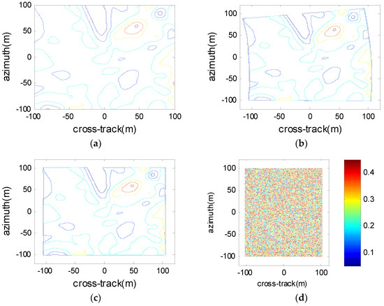
Figure 15.
Topographic profile: (a) The topographic profile of the ideal scene; (b) the topographic profile before deformation correction; (c) the topographic profile after deformation correction; and (d) the errors of the corresponding positions in Figure 15a,c.
7. Conclusions
In the DLSLA 3D SAR imaging model with yaw angle, the Doppler frequency modulation is spatial-variant, and is related to the modulated cross-track coordinates rather than the modulated azimuth coordinates, and the focused 3D image will be deformed in the azimuth and cross-track plane. In this paper, we propose a method to estimate platform motion parameters, which can be used to construct compensation functions to compress azimuth signal and compensate for motion error of the platform. The deformation correction of focused 3D image can be realized by the deformation correction procedure. It must be mentioned that the proposed method can also be extended to the applications of multi-input multi output (MIMO) radar systems, although the current paper analyzed a single transmitter element for clarity. In MIMO array, it is necessary to compensate for the error introduced by the EPC, which is related to the platform velocity. We will consider how to compensate for motion errors in the MIMO array in the future work.
Author Contributions
Conceptualization, Q.L. and Q.Z.; Data curation, W.H.; Funding acquisition, Y.L., Q.Z. and T.S.Y.; Investigation, Q.L.; Methodology, Q.L.; Resources, Q.Z. and W.H.; Supervision, T.S.Y.; Validation, Y.L.; Writing—original draft, Q.L. and Y.L.; Writing—review & editing, T.S.Y.
Funding
This research was funded by the National Natural Science Foundation of China under Grant No. 61471386 and 61571457; the Ministry of Education, Singapore under Grant No. MOE2016-T2-1-070; and the China Scholarship Council (CSC) under Grant No. 201703170012.
Acknowledgments
The authors would like to thank the handing Associate Editor and the anonymous reviewers for their valuable comments and suggestions for this paper.
Conflicts of Interest
The authors declare no conflicts of interest.
Appendix A
In this appendix, we will derive the calculation of and .
Firstly, we derive the derivative of plural modulus. For plurality , where is the real part, is the imaginary part, and is a variable. The plural modulus can be obtained by . The first-order derivative of to variable is:
then, the first-order derivative of to η can be obtained by:
where and are the real and imaginary parts of , respectively. Meanwhile, the element is:
where and represent the mth row and qth column element of matrices and , respectively. and represent the qth element of vectors and , respectively. , and are known. Denote:
where and are the real and imaginary parts of , respectively. Meanwhile, the compensation function can expressed as , where . Then:
According to Equation (40), the real part and the imaginary part of can be expressed as:
then, the first and second derivatives of and can be obtained by the following equations:
where ,. Then, and can be calculated, and can be obtained.
References
- Klare, J.; Cerutti, D.; Brenner, A.; Ender, J. Image quality analysis of the vibrating sparse MIMO antenna array of the airborne 3D imaging radar ARTINO. In Proceedings of the IEEE International Geoscience and Remote Sensing Symposium (GRASS), Barcelona, Spain, 23–28 July 2007; pp. 5310–5314. [Google Scholar]
- Lin, Y.; Hong, W.; Tan, W.X.; Wu, Y.R. Extension of rangemigration algorithm to squint circular SAR imaging. IEEE Geosci. Remote Sens. Lett. 2011, 8, 651–655. [Google Scholar] [CrossRef]
- Zhu, X.X.; Bamler, R. Very High Resolution Spaceborne SAR Tomography in Urban Environment. IEEE Trans. Geosci. Remote Sens. 2010, 48, 4296–4308. [Google Scholar] [CrossRef]
- Reigber, A.; Moreira, A. First Demonstration of Airborne SAR Tomography Using Multibaseline L-Band Data. IEEE Trans. Geosci. Remote Sens. 2000, 38, 2142–2152. [Google Scholar] [CrossRef]
- Liang, L.; Li, X.W.; Ferro-Famil, L.; Guo, H.D.; Zhang, L.; Wu, W.J. Urban area tomography using a sparse representation based two-dimensional spectral analysis technique. Remote Sens. 2018, 10, 109. [Google Scholar] [CrossRef]
- Shi, J.; Zhang, X.L.; Yang, J.Y.; Wang, Y.B. Surface-tracing-based LASAR 3-D imaging method via multiresolution approximation. IEEE Trans. Geosci. Remote Sens. 2008, 46, 3719–3730. [Google Scholar] [CrossRef]
- Han, K.Y.; Wang, Y.P.; Tan, W.X.; Hong, W. Efficient pseudopolar format algorithm for down-looking linear-array SAR 3-D imaging. IEEE Geosci. Remote Sens. Lett. 2015, 12, 572–576. [Google Scholar] [CrossRef]
- Du, L.; Wang, Y.P.; Hong, W.; Tan, W.X.; Wu, Y.R. A three-dimensional range migration algorithm for downward-looking 3-D-SAR with single-transmitting and multiple-receiving linear array antennas. EURASIP J. Adv. Signal Process 2010, 957916, 1–15. [Google Scholar] [CrossRef]
- Liu, Q.Y.; Zhang, Q.; Gu, F.F.; Cheng, Y.C.; Kang, L.; Qu, X.Y. Downward-looking linear array 3D SAR imaging based on multiple measurement vectors model and continuous compressive sensing. J. Sens. 2017, 2017, 6207828. [Google Scholar] [CrossRef]
- Zhang, S.Q.; Zhu, Y.T.; Kuang, G.Y. Imaging of downward-looking linear array three-dimensional SAR based on FFT-MUSIC. IEEE Geosci. Remote Sens. Lett. 2015, 12, 885–889. [Google Scholar] [CrossRef]
- Wei, S.J.; Zhang, X.L.; Shi, J.; Liao, K.F. Sparse array microwave 3-D imaging: Compressed sensing recovery and experimental study. Progr. Electromagn. Res. 2012, 135, 161–181. [Google Scholar] [CrossRef]
- Peng, X.M.; Tan, W.X.; Wang, Y.; Hong, W.; Wu, Y.R. Convolution back-projection imaging algorithm for downward-looking sparse linear array three dimensional synthetic aperture radar. Prog. Electromagn. Res. 2012, 129, 287–313. [Google Scholar] [CrossRef]
- Chen, C.; Zhang, X. A new super-resolution 3-D SAR imaging method based on MUSIC algorithm. In Proceedings of the IEEE RadarCon (RADAR), Kansas, MO, USA, 23–27 May 2011; pp. 525–529. [Google Scholar]
- Gu, F.F.; Zhang, Q.; Chi, L.; Cheng, Y.A.; Li, S. A Novel motion compensating method for mimo-sar imaging based on compressed sensing. IEEE Sens. J. 2015, 15, 2157–2165. [Google Scholar] [CrossRef]
- Donoho, D.L. Compressed sensing. IEEE Trans. Inf. Theory 2006, 52, 1289–1306. [Google Scholar] [CrossRef]
- Cand´es, E.J.; Wakin, M.B. An introduction to compressive sampling. IEEE Signal Process. Mag. 2008, 25, 21–30. [Google Scholar] [CrossRef]
- Kwak, N. Principle component analysis based on L1 norm maximization. IEEE Trans. Pattern Anal. Mach. Intell. 2008, 30, 1672–1680. [Google Scholar] [CrossRef] [PubMed]
- Peng, X.M.; Tan, W.X.; Hong, W.; Jiang, C.L.; Bao, Q.; Wang, Y.P. Airborne SLADL 3-D SAR image reconstruction by combination of polar formatting and L1 regularization. IEEE Trans. Geosci. Remote Sens. 2016, 54, 213–226. [Google Scholar] [CrossRef]
- Zhang, S.Q.; Zhu, Y.T.; Dong, G.G.; Kuang, G.Y. Truncated SVD-based compressive sensing for downward-looking three-dimensional sar imaging with uniform/nonuniform linear array. IEEE Geosci. Remote Sens. Lett. 2015, 12, 1853–1857. [Google Scholar] [CrossRef]
- Tang, G.G.; Bhaskar, B.N.; Shah, P.; Recht, B. Compressed sensing off the grid. IEEE Trans. Inf. Theory 2013, 59, 7465–7490. [Google Scholar] [CrossRef]
- Yang, Z.; Xie, L.H. Enhancing sparsity and resolution via reweighted atomic norm minimization. IEEE Trans. Signal Process. 2016, 64, 1–12. [Google Scholar] [CrossRef]
- Bao, Q.; Han, K.Y.; Peng, X.M.; Hong, W.; Zhang, B.C.; Tan, W.X. DLSLA 3-D SAR imaging algorithm for off-grid targets based on pseudo-polar formatting and atomic norm minimization. Sci. China 2016, 59, 062310. [Google Scholar] [CrossRef]
- Liu, Q.Y.; Zhang, Q.; Luo, Y.; Li, K.M.; Sun, L. Fast algorithm for sparse signal reconstruction based on off-grid model. IET Radar Sonar Navig. 2018, 12, 390–397. [Google Scholar] [CrossRef]
- Wu, Z.B.; Zhu, Y.T.; Su, Y.; Li, Y.; Song, X.J. MIMO array design for airborne linear array 3D SAR imaging. J. Electron. Inf. Technol. 2013, 35, 2672–2677. [Google Scholar] [CrossRef]
- Bao, Q.; Jiang, C.L.; Lin, Y.; Tan, W.X.; Wang, Z.R.; Hong, W. Measurement matrix optimization and mismatch problem compensation for DLSLA 3-D SAR cross-track reconstruction. Sensors 2016, 16, 1333. [Google Scholar] [CrossRef] [PubMed]
- Zhang, S.Q.; Dong, G.G.; Kuang, G.Y. Superresolution downward-looking linear array three-dimensional SAR imaging based on two-dimensional compressive sensing. IEEE J. Sel. Top. Appl. Earth Obs. Remote Sens. 2016, 9, 2184–2196. [Google Scholar] [CrossRef]
- Ren, X.; Chen, L.; Yang, T. 3D imaging algorithm for down-looking MIMO array SAR based on Bayesian compressive sensing. Int. J. Antennas Propag. 2014, 2014, 612326. [Google Scholar] [CrossRef]
- Yang, Z.M.; Sun, G.C.; Xing, M.D.; Bao, Z. motion compensation for airborne 3-D SAR based on joint multi-channel auto-focusing technology. J. Electron. Inf. Technol. 2012, 34, 1581–1588. [Google Scholar] [CrossRef]
- Ding, Z.Y.; Tan, W.X.; Wang, Y.P.; Hong, W.; Wu, Y.R. Yaw angle error compensation for airborne 3-D SAR based on wavenumber-domain subblock. J. Radars 2015, 4, 467–473. [Google Scholar] [CrossRef]
- Macedo, K.A.C.D.; Scheiber, R. Precise tomography and aperture dependent motion compensation for airborne SAR. IEEE Geosci. Remote Sens. Lett. 2005, 2, 172–176. [Google Scholar] [CrossRef]
- Xing, M.D.; Jiang, X.W.; Wu, R.B.; Zhou, F.; Bao, Z. Motion compensation for UAV SAR based on raw radar data. IEEE Trans. Geosci. Remote Sens. 2009, 47, 2870–2883. [Google Scholar] [CrossRef]
- Du, L.; Wang, Y.P.; Hong, W.; Wu, Y.R. Analysis of 3D-SAR based on angle compression principle. In Proceedings of the International Geoscience and Remote Sensing Symposium (IGARSS), Boston, MA, USA, 7–11 July 2008; pp. 1324–1327. [Google Scholar]
- Li, J.; Stoica, P.; Zhen, X.Y. Signal Synthesis and Receiver Design for MIMO Radar Imaging. IEEE Signal Process. 2008, 56, 3959–3968. [Google Scholar] [CrossRef]
- Wang, L.B.; Xu, J.; Huang, F.K.; Peng, Y.N. Analysis and Compensation of Equivalent Phase Center Error in MIMO-SAR. Acta Electron. Sin. 2009, 12, 2687–2693. [Google Scholar] [CrossRef]
- Chen, Y.; Li, G.; Zhang, Q.; Zhang, Q.J.; Xia, X.G. Motion compensation for airborne SAR via parametric sparse representation. IEEE Trans. Geosci. Remote Sens. 2017, 55, 551–562. [Google Scholar] [CrossRef]
- Fan, B.K.; Ding, Z.G.; Gao, W.B.; Long, T. An improved motion compensation method for high resolution UAV SAR imaging. Sci. China 2014, 57, 122301:1–122301:13. [Google Scholar] [CrossRef]
- Lin, Y.; Hong, W.; Tan, W.X.; Wang, Y.P.; Xiang, M.S. Airborne circular SAR imaging: Results at P-band. In Proceedings of the International Geoscience and Remote Sensing Symposium (IGARSS), Munich, Germany, 22–27 July 2012; pp. 5594–5597. [Google Scholar]
© 2018 by the authors. Licensee MDPI, Basel, Switzerland. This article is an open access article distributed under the terms and conditions of the Creative Commons Attribution (CC BY) license (http://creativecommons.org/licenses/by/4.0/).