Article

Hyperspectral Mixed Denoising via Spectral Difference-Induced Total Variation and Low-Rank Approximation †

1
School of Computer and Software, Nanjing University of Information Science and Technology, Nanjing 210044, China
2
Key Laboratory of Intelligent Perception and Systems for High-Dimensional Information of Ministry of Education, Nanjing University of Science and Technology, Nanjing 210094, China
3
School of Information Engineering, Nanjing Audit University, Nanjing 211815, China
4
School of Computer Science and Engineering, Nanjing University of Science and Technology, Nanjing 210094, China
5
Department of Electrical and Computer Engineering, Sungkyunkwan University, Suwon 440746, Korea
*
Author to whom correspondence should be addressed.
This paper is an extension of our IWAIT conference paper.
Remote Sens. 2018, 10(12), 1956; https://doi.org/10.3390/rs10121956
Submission received: 9 November 2018 / Revised: 28 November 2018 / Accepted: 4 December 2018 / Published: 5 December 2018
(This article belongs to the Section Remote Sensing Image Processing)

Abstract

:
Exploration of multiple priors on observed signals has been demonstrated to be one of the effective ways for recovering underlying signals. In this paper, a new spectral difference-induced total variation and low-rank approximation (termed SDTVLA) method is proposed for hyperspectral mixed denoising. Spectral difference transform, which projects data into spectral difference space (SDS), has been proven to be powerful at changing the structures of noises (especially for sparse noise with a specific pattern, e.g., stripes or dead lines present at the same position in a series of bands) in an original hyperspectral image (HSI), thus allowing low-rank techniques to get rid of mixed noises more efficiently without treating them as low-rank features. In addition, because the neighboring pixels are highly correlated and the spectra of homogeneous objects in a hyperspectral scene are always in the same low-dimensional manifold, we are inspired to combine total variation and the nuclear norm to simultaneously exploit the local piecewise smoothness and global low rankness in SDS for mixed noise reduction of HSI. Finally, the alternating direction methods of multipliers (ADMM) is employed to effectively solve the SDTVLA model. Extensive experiments on three simulated and two real HSI datasets demonstrate that, in terms of quantitative metrics (i.e., the mean peak signal-to-noise ratio (MPSNR), the mean structural similarity index (MSSIM) and the mean spectral angle (MSA)), the proposed SDTVLA method is, on average, 1.5 dB higher MPSNR values than the competitive methods as well as performing better in terms of visual effect.

Graphical Abstract

1. Introduction

Hyperspectral images (HSIs) contain a broad range of spectral information from 400 nm to 2500 nm which can provide a rich observation capability beyond human vision. This enables HSIs to be widely used in many applications [1], e.g., precision agriculture, pharmaceutical, medical diagnosis, and food security. However, in the course of data acquisition, the HSIs are often degraded by multiple noises, such as Gaussian noise and sparse noise (including impulse noise, stripe noise and dead lines). It significantly decreases the accuracy of subsequent applications, e.g., classification [2,3,4], target detection [5] and unmixing [6,7]. Therefore, it is necessary and important to develop more effective noise reduction techniques for HSIs.
To date, enormous approaches have been developed for HSI denoising. For instance, in the framework of Bayesian inferring, noise-adjusted principal component (NAPC) analysis [8] and minimum noise fraction (MNF) [9] are the representative denoising methods for HSIs and both have been successfully applied to ENVI and EDARS software. Besides, by treating an HSI as the combination of gray images, lots of traditional methods, e.g., bilateral filtering [10], total variation [11], nonlocal means [12] and convolutional networks [13], can be directly applied to recover HSI data. However, due to lack of the consideration of spectral correlations, these methods often result in unsatisfactory performance.
Being good at learning and representing multi-scale information of signals with few atoms, wavelet methods [14] have become another powerful instrument for HSI denoising. Sparse regularizations, e.g., Lasso penalty [15] or l 1 sparsity [16], are always combined with wavelet transform for image denoising. In [17,18], principal component analysis (PCA) was combined with a 3D or 4D wavelet filtering to get rid of the Gaussian noise in the low-energy channels and improved the denoising performance. In [19], a novel wavelet-based sparse reduced-rank regression (WSRRR) method, in which the tuning parameters were adaptively calculated based on Stein’s unbiased risk estimation, was introduced for Gaussian noise reduction of HSI. To further reduce the computational complexity, a parameter-free method for the restoration of HSIs termed HyRes [20] was proposed. It introduced a sparse low-rank model by fixing the orthogonal projection instead of updating it iteratively, thus estimating the unknown signal in the subspace and saving the time. In addition to wavelet technique, sparse representation (SR) is also popular for HSI denoising, due to its powerful capacity of linearly representing signals with few basis [21]. It makes a great consistence with the linear mixture assumption that spectra in HSIs all lie in a subspace linearly spanned by the spectra of endmembers. In [22], a novel HSI denoising method was proposed to use the global and local redundancy and correlation (RAC) in spectral and spatial domains. While in [23], a novel spectral-spatial distributed SR method was put forward for HSI denoising. It exploited both intraband and interband structures in the course of learning. To fully use the highly correlated spectral information and similar spatial information, a novel spatial and spectral adaptive SR (SSASR) method [24] was introduced to further improve the performance of estimation. More literatures for HSI denoising related to SR or dictionary learning can be found in [25,26,27] and therein references. Moreover, deep learning, as one of the powerful nonlinear feature extraction and signal representation techniques [28,29,30], have gradually emerged in HSI denoising and achieved considerable results [31,32].
Recently, low-rank techniques have drawn increased attention and become one of the powerful tools in exploiting the intrinsic properties of HSIs. A multitude of remarkable methods have been proposed for HSI denoising in the framework of low-rank approximation. For example, a novel destriping method via low-rank representation (LRR) was introduced for HSI [33]. It employed global LRR for exploring the highly correlated spectral information between bands and enforced a graph constraint to preserve the local details. Later, Zhang et al. [34] proposed to employ low-rank matrix recovery (LRMR) for HSI mixed noise removal by “GoDec” algorithm [35] and achieved significant success. However, LRMR has one obvious weakness that it only considers the local similarity within local patches and ignores the unbiased noise intensity in each patch. To alleviate such problem, the spectrally nonlocal LRR [36], group LRR [37], noise adaptive estimation [38] and subspace LRR [39] were put forward to further explore more useful information of HSI and improve the performance. Meanwhile, several tensor low rank (TLR)-based methods [40,41,42] are also proposed to exploit the spatial-spectral structures in overlapped cubic tensors. Compared to LR methods, those TLR methods only modify to exploit the low-rank property from a 2d matrix manner to a 3d tensor manner, thus further improving the denoising performance to an extent. However, there are still two fatal flaws for those pure LR or TLR-based methods. First, because of the independent distribution of Gaussian noise, LR or TLR methods are not excellent at getting rid of them completely. Second, either LR or TLR methods cannot completely get rid of the structured stripes and dead lines, that is, when they present at the same position in a series of bands, pure LR or TLR approaches would treat them as low-rank features and retain them.
These two shortcomings severely limit the denoising accuracy of LR and TLR methods. To alleviate these limitations, other techniques that explore more additional information should be involved for further improvement. Total variation (TV) which has been demonstrated as an effective tool for Gaussian noise removal, should be one of the best candidates. Recently, band-by-band TV [43], 3-dimensional TV (3DTV) [44,45], and tensor TV (TenTV) [46] have been involved into the framework of LR and TLR framework for HSI mixed denoising. Although these three types of algorithms could significantly improve the precision of HSI mixed denoising, they still cannot completely get rid of the sparse noise with a specific pattern. The reason may be that TV regularizer is prone to enforce the pixel differences along horizontal and vertical directions, and one of the two directions just coincides with the direction of the stripes or dead lines. It means that the TV defined in each band (e.g., band-by-band TV and TenTV) would maintain the structure of stripes or dead lines along the horizontal or vertical direction. Benefitting from the spectral difference constraint, 3DTV can assist LRR [45] or TLR [47] techniques to remove the structured sparse noise to an extent; however, it will lead, more or less, to spectral distortion. More recently, a novel HSI denoising method which enforces LRR on the spectral difference space (LRRSDS) [48] has achieved great attention in suppressing the structured sparse noise. It can change the structures of noises by projecting them into the SDS, and then remove them effectively with LR techniques. However, one shortcoming for LRRSDS is that it does not take the spatially local correlations into consideration, thus failing to remove the heavy Gaussian noise completely.
By taking full consideration of the above three techniques (i.e., TV, LRR and SDS), in this paper, we propose a novel spectral difference-induced TV and low-rank approximation method, termed SDTVLA, for HSI mixed denoising, and the flowchart of it is illustrated in Figure 1. It needs to be noted that this manuscript is extended from our conference paper [49] and the contributions are summarized as follows.
  • The proposed method takes full consideration of three kinds of noises that exist in HSI, i.e., random sparse noise, Gaussian noise, and structured sparse noises. To completely remove all of them, multiple priors (TV, LRR and SDS) are fused into a unified framework to accurately reconstruct the underlying clean HSI.
  • The combination of TV and SDS can be treated as a novel cross TV (CTV) which is defined as the conventional 2-d TV across one-dimensional spectral TV, and CTV has been validated to be effective for dealing with both Gaussian noise and structured stripes.
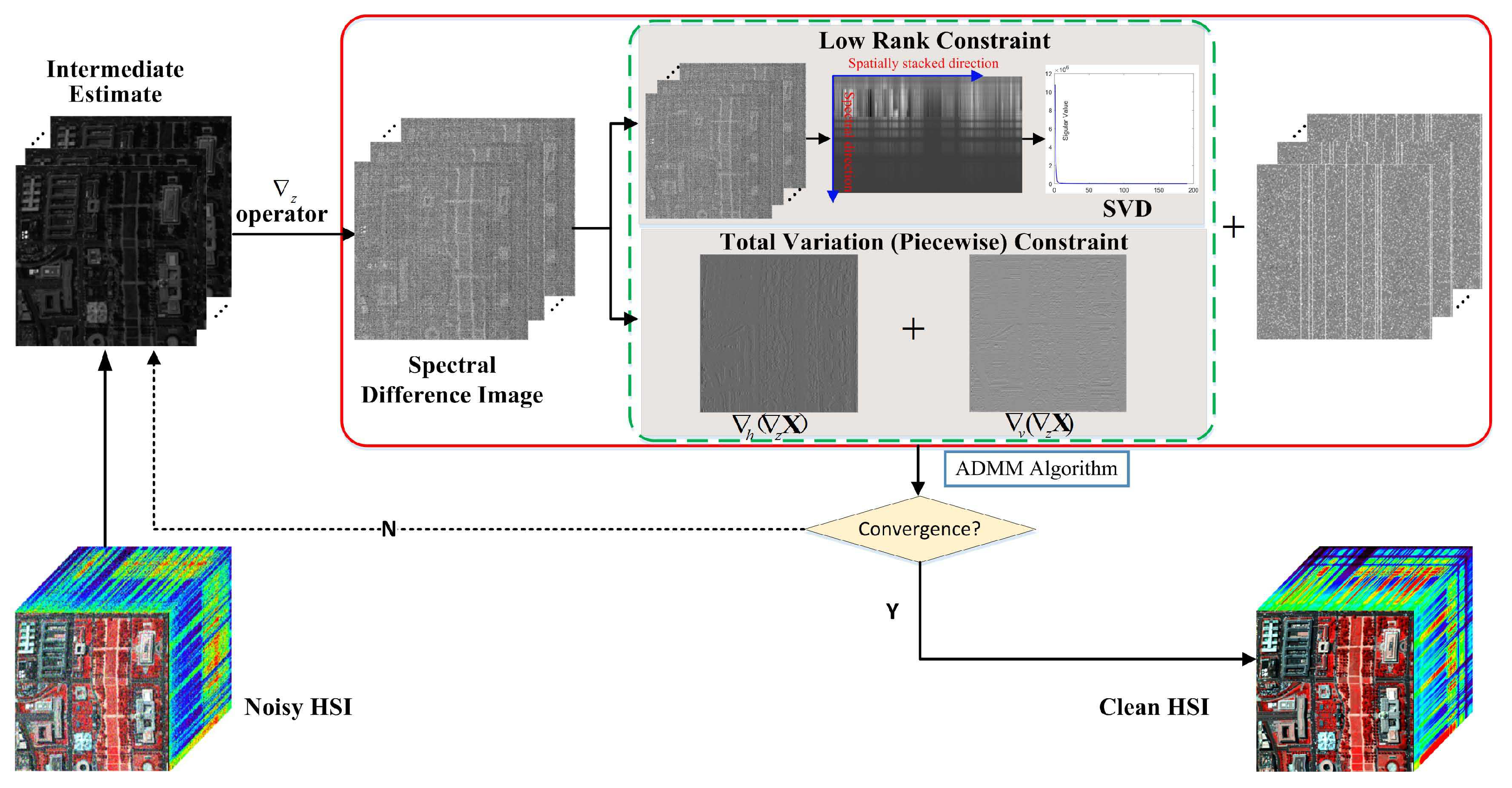
  • The SDTVLA model with all convex terms is easy to be separately solved by alternating direction method of multipliers (ADMM).
  • Extensive experiments on three simulated and two real HSI datasets demonstrate the superiority of SDTVLA algorithm in terms of visual effect and quantitative assessment.
The remainder of this paper is organized as follows. Section 2 recalls the related works of two state-of-the-art LR-based methods. Section 3 formulates the newly developed denoising method via spectral difference-induced TV and low-rank approximation. Section 4 presents the experimental results and discussions on simulated and real HSI datasets as well as the parameters analysis. Conclusions are drawn in Section 5.

2. Background Formulation

2.1. Observation Model

Before formulating the problems for HSI denoising, we make some notations as follows. Let  Y R ( m × n ) × l (2-d matrix reshaped from the 3-d tensor Y R m × n × l ) be the observed noisy HSI with m × n pixels and l bands, and let X R ( m × n ) × l represent the latent noise-free HSI. In the mixed noise scenario, the observation model for HSI can be formulated in a matrix form as
Y = X + S + N
where S R ( m × n ) × l denotes sparse noise in the scene and N R ( m × n ) × l represents the Gaussian noise generated by the sensor or atmospheric effect.

2.2. LRMR Model

Having (1) in mind, the LRMR model for HSI mixed denoising can be expressed as [34]:
min X , S | | Y X S | | F 2 + λ 1 | | S | | 1 + λ 2 | | X | | *
where | | S | | 1 = | s i | is the l 1 norm of the sparse noise matrix S and s i denotes the i-th element of X . | | X | | * denotes the well-known nuclear norm and it is defined as the sum of the absolute values of all singular values, i.e.,  | | X | | * = | σ i | .
Due to the simplicity and good performance for mixed noise reduction, the model (2) and its variants have evolved into one of the fundamental models. In [34], the model (2) was equivalently rewritten as the following formulation.
min X , S | | Y X S | | F 2 , s . t . , c a r d ( S ) k c a r d , r a n k ( X ) r
where c a r d ( · ) denotes the cardinality of S , and r a n k ( · ) represents the low-rank constraint. The model (3) can be effectively and easily solved by “GoDec” algorithm [35].
As analyzed in Section 1, LRMR cannot successfully recover the data with severe Gaussian noise and structured stripes. Take Figure 2 for example, it is easy to see that LRMR produces a satisfactory result for the band 103 with moderate noise level (see Figure 2a) while it fails to get rid of the heavy Gaussian noise and structured stripes in band 108, see Figure 2b.

2.3. LRTV Model

To alleviate the shortcoming of LRMR, the LRTV model [43] which combines band-by-band TV regularization and low-rank constraint together was put forward to further improve the denoising accuracy. It aims at solving the optimization problem as
min X , S | | X | | * + λ | | S | | 1 + τ | | X | | HTV s . t . | | Y X S | | F 2 ε , r a n k ( X ) r
where | | X | | HTV is the so-called ’hyperspectral total variation’ which enforces the conventional TV constraint in each band and is defined as:
| | X | | HTV = i l | | H X i | | TV = i l { | | h X i | | 1 + | | v X i | | 1 } | | h X | | 1 + | | v X | | 1
where X i is the vectorization of the i-th band image. H : R ( m × n ) × 1 R m × n is defined as an operator to reshape the one-dimensional vector into a 2D image, h and v can be seen as two convolution operators in the horizontal and vertical directions, respectively. Thanks to the HTV term, LRTV can yield much superior performance than LRMR, especially for getting rid of the severe Gaussian noise. However, neither LRTV nor LRMR can effectively get rid of the structured stripes completely. Take Figure 2 for instance, LRTV produces the cleaner result than LRMR method in moderate noise case, see Figure 2c. However, for band 108 with severe Gaussian noise and structured stripes, LRTV fails to remove them, see Figure 2d.

3. Proposed SDTVLA Method

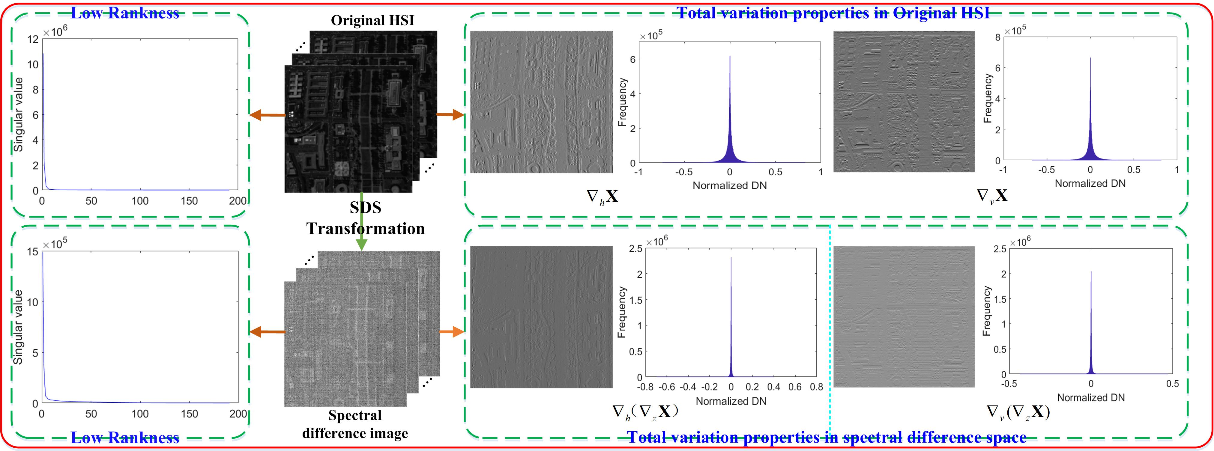
3.1. Spectral Difference Transformation

First, we give the definition of spectral difference transformation [48]. It aims at projecting the original data into the spectral difference image and then recovering the image from the residual space.
z X ( : , i ) = X ( : , i ) X ( : , i 1 ) , f o r 2 i l 0 , f o r i = 1
where X ( : , i ) denotes the i-th column of X , and it is also the vectorization of the i-th band image of the HSI.
According to the above definition, spectral difference transform is a linear projection. It will not change the distribution of Gaussian noise and impulse noise except for slightly changing the intensities of them. However, these changes can be alleviated by adjusting the related parameters in the proposed model. As analyzed in [48], the advantage of SDS is that it will change the patterns of the structured stripes and dead lines, so that the LR technique can be used to effectively remove them.
Moreover, by comparing the low rankness and total variation properties in SDS with those in the original HSI space, we find that the TV in SDS would promote much strong sparsity than that in the original HSI, see Figure 3, while the low rankness in SDS shows similar behavior as that in the original HSI space. Therefore, it inspires us to employ both in SDS to further improve the performance of HSI mixed denoising.

3.2. SDTVLA Model

Based on the above analysis, a novel spectral difference-induced TV regularization and low-rank approximation method is put forward for HSI mixed denoising and it aims at dealing with the optimization problem as:
min X , S | | Y X S | | F 2 + λ 1 | | S | | 1 + λ 2 | | z X | | * , TV s . t . r a n k ( z X ) r
where | | z X | | * , TV is the novel combination term, which simultaneously exploits the local piecewise smoothness by the TV constraint and the global low rankness by the nuclear norm in SDS. It is defined as follows.
| | z X | | * , TV = | | z X | | * + ρ | | z X | | TV
where ρ is a parameter that keeps the balance of TV regularization and low-rank constraint in SDS. | | z X | | TV = | | h ( z X ) ) | | 1 + | | v ( z X ) ) | | 1 , here z is the spectral difference transform. Parameters λ 1 and λ 2 control the tradeoff between the sparse noise term and the combination term.
The advantages of model (7) can be summarized as follows.
  • Different from the conventional TV constraint in each band, here the TV regularization is defined in SDS, and it can be seen as a cross TV that explores both spatial and spectral information. Meanwhile, it could effectively help low-rank tools to reduce the severe Gaussian noise and structured stripes.
  • Spectral difference transform can effectively change the structures of the noises in the original HSI, thus enabling the TVLA regularization to further improve the denoising accuracy of the structured stripes.
  • With all convex regularizations, the model (7) can be effectively and easily solved by ADMM.

3.3. Optimization

In this subsection, ADMM is used to effectively solve the optimization problem (7) by spitting it into several simpler subproblems. By introducing the auxiliary variables Q 1 = z X , Q 2 = z X , Q 3 = h Q 2 and Q 4 = v Q 2 , the Lagrangian function of problem (7) can be expressed as
( X , S , Q 1 , . . , Q 4 ) = | | Y X S | | F 2 + λ 1 | | S | | 1 + λ 2 { | | Q 1 | | * + ρ ( | | Q 3 | | 1 + | | Q 4 | | 1 ) } + μ | | Q 1 z X B 1 | | F 2 + μ | | Q 2 z X B 2 | | F 2 + μ | | Q 3 h Q 2 B 3 | | F 2 + μ | | Q 4 v Q 2 B 4 | | F 2 s . t . r a n k ( Q 1 ) r
where B 1 , B 2 , B 3 , B 4 are four augmented multipliers and μ > 0 is the regularization parameter.
Generally, we minimize the Lagrangian function (9) iteratively over one variable while fixing the other ones. Algorithm 1 summarizes the main steps for solving the proposed SDTVLA model using ADMM.
Algorithm 1 The pseudo-code for SDTVLA solver via ADMM.
1:
Input: The noisy HSI Y , λ 1 0 , λ 2 0 , rank r > 0 and the maximum iteration k m a x .
2:
Initialization S ( 0 ) = 0 , X ( 0 ) = 0 , Q 1 ( 0 ) = Q 2 ( 0 ) = Q 3 ( 0 ) = Q 4 ( 0 ) = 0 , B 1 ( 0 ) = B 2 ( 0 ) = B 3 ( 0 ) = B 4 ( 0 ) = 0 , ρ = 0.5 , μ = 1.0 , and current iteration k = 0
3:
For k k m a x do
4:
       X ( k + 1 ) = argmin X ( X , S ( k ) , Q i ( k ) , B i ( k ) ) , i = 1 , 2
5:
       S ( k + 1 ) = softTH ( Y X ( k + 1 ) , λ 1 )
6:
       Q i ( k + 1 ) = argmin Q i ( X ( k + 1 ) , S ( k + 1 ) , Q i , B i ( k ) ) , i = 1 , 2 , 3 , 4
7:
   Update Lagrangian multipliers
8:
       B 1 ( k + 1 ) B 1 ( k ) + z X ( k + 1 ) Q 1 ( k + 1 )
9:
       B 2 ( k + 1 ) B 2 ( k ) + z X ( k + 1 ) Q 2 ( k + 1 )
10:
       B 3 ( k + 1 ) B 3 ( k ) + h Q 2 ( k + 1 ) Q 3 ( k + 1 )
11:
       B 4 ( k + 1 ) B 4 ( k ) + v Q 2 ( k + 1 ) Q 4 ( k + 1 )
12:
   Update iteration k = k + 1
13:
End For
14:
Output: The latent noise-free HSI X .
Line 4 in Algorithm 1 is to solve the X subproblem as follows.
X ( k + 1 ) = argmin X | | Y X S ( k ) | | F 2 + μ | | Q 1 ( k ) z X B 1 ( k ) | | F 2 + μ | | Q 2 ( k ) z X B 2 ( k ) | | F 2
Optimization problem (10) is a quadratic programming problem and has an analytical solution by the n-dimensional fast Fourier transform (nFFT).
X ( k + 1 ) = F 1 F ( Y S ( k ) + μ z T ( ξ 1 ( k ) ) + μ z T ( ξ 2 ( k ) ) 1 + 2 μ F ( z ) H F ( z ) ,
where ξ 1 ( k ) = Q 1 ( k ) B 1 ( k ) , ξ 2 ( k ) = Q 2 ( k ) B 2 ( k ) , F 1 is the inverse nFFT operator, F is the nFFT operator, and H represents complex conjugate.
Line 5 in Algorithm 1 is to solve the S subproblem.
S ( k + 1 ) = argmin S | | Y X ( k + 1 ) S | | F 2 + λ 1 | | S | | 1 .
Optimization problem (12) can be effectively solved by the well-known soft-thresholding function.
S = softTH ( W , λ 1 ) = sign ( W ) max { 0 , | W | λ 1 2 } ,
where W = Y X ( k + 1 ) , and sign ( · ) is an odd function that extracts the sign of a real number.
Line 6 in Algorithm 1 is to solve the subproblems regarding the auxiliary variables Q i , i = 1 , 2 , 3 , 4 [50,51]. In the following, we will show the details for solving the corresponding subproblems.
The optimization subproblem related to variable Q 1 can be expressed as:
Q 1 ( k + 1 ) = argmin r a n k ( Q 1 ) r λ 2 | | Q 1 | | * + μ | | Q 1 z X ( k + 1 ) B 1 ( k ) | | F 2
Problem (14) is a nuclear norm minimization problem, which can be easily solved by the famous singular-value thresholding operator, and the solution can be expressed as follows.
Q 1 ( k + 1 ) = D λ 2 2 μ z X ( k + 1 ) + B 1 ( k ) , r
where
D λ ( Z ) = U D λ ( Σ r ) V T = U diag max ( σ i λ , 0 ) 1 i r V T ,
Z = U Σ V T is the singular-value decomposition, and { σ i } 1 i r are the first r largest singular values of matrix Z .
The optimization problem related to variable Q 2 is similar to that of X , and it is also a quadratic programming problem.
Q 2 ( k + 1 ) = argmin Q 2 μ | | Q 2 z X ( k + 1 ) B 2 ( k ) | | F 2 + μ | | Q 3 ( k ) h Q 2 B 3 ( k ) | | F 2 + μ | | Q 4 ( k ) v Q 2 B 4 ( k ) | | F 2
The equivalent linear system of the model (17) can be express as:
( I + Δ ) Q 2 ( k + 1 ) = z X ( k + 1 ) + B 2 ( k ) + h T ( ξ 3 ( k ) ) + v T ( ξ 4 ( k ) )
where Δ = h T h + v T v , ξ 3 ( k ) = Q 3 ( k ) B 3 ( k ) , ξ 4 ( k ) = Q 4 ( k ) B 4 ( k ) .
Regarding h and v as two convolutions along spatial directions, problem (17) has the closed form solution by using fast nFFT operator.
Q 2 ( k + 1 ) = F 1 F z X ( k + 1 ) + B 2 ( k ) + h T ( ξ 3 ( k ) ) + v T ( ξ 4 ( k ) ) 1 + F ( h ) H F ( h ) + F ( v ) H F ( v )
For the remaining two variables, i.e., Q 3 and Q 4 , the optimization subproblems related to them have the same mathematical form. That is, both can be effectively solved by the soft-thresholding function which has been given in (13).
Q 3 ( k + 1 ) = softTH ( h Q 2 + B 3 ( k ) , λ 2 ρ / 2 μ ) Q 4 ( k + 1 ) = softTH ( v Q 2 B 4 ( k ) , λ 2 ρ / 2 μ )

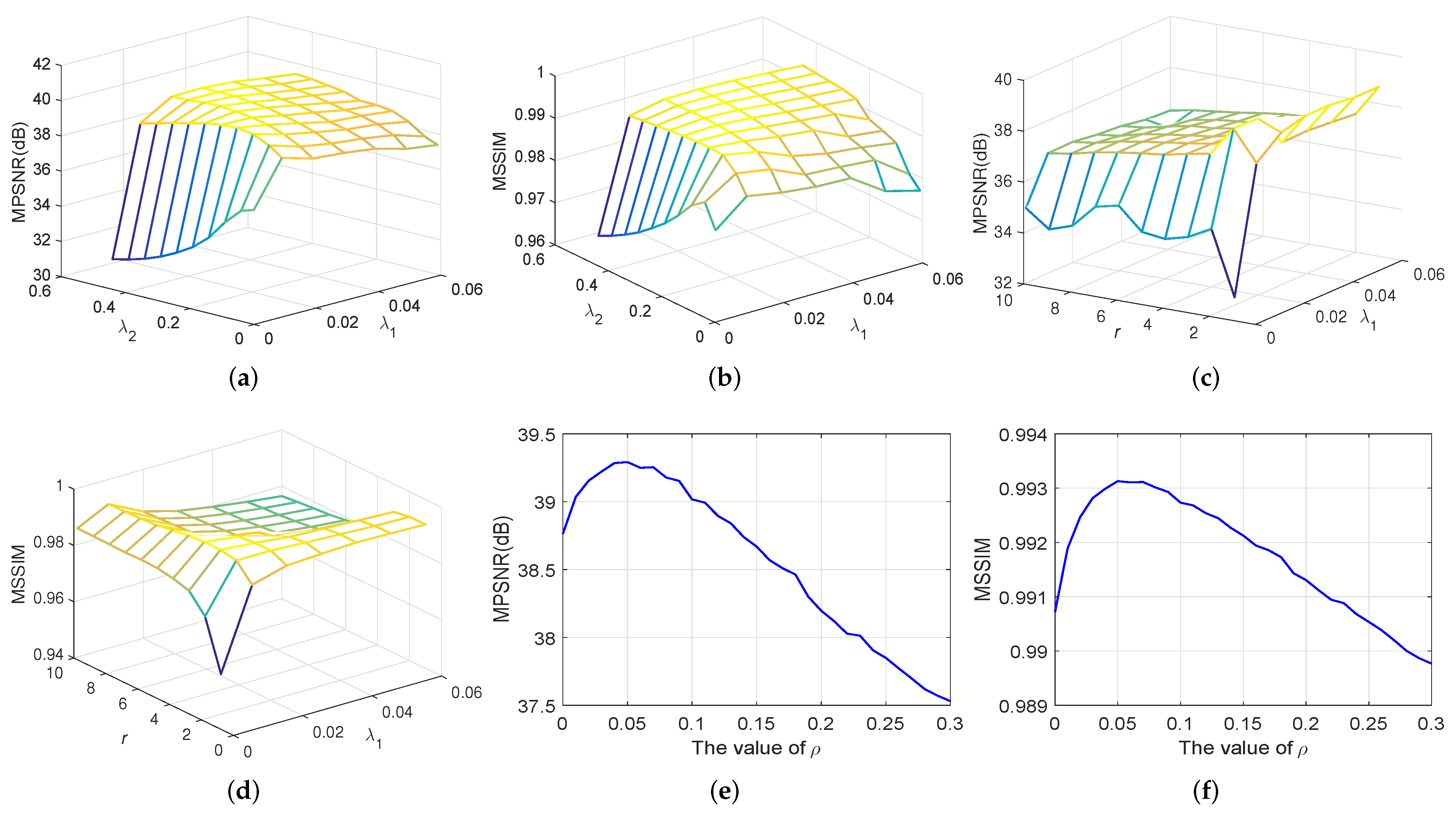
3.4. Parameters Determination and Convergence Analysis

There are totally four parameters, i.e., λ 1 , λ 2 , ρ and the latent rank r, in SDTVLA solver. As analyzed above, parameter λ 1 has a strong relationship to the intensity of sparse noise in HSI. Empirically, we set it as λ 1 = 10 m × n by default in the following experiments, here n and m are dimensions of the image in each band of HSI. λ 2 is the combined regularizer’s parameter, which controls the contribution of the low-rank and total variation constraints in SDS while ρ is the proportion parameter related to the cross TV regularizer. Later, we will systematically discuss and analyze the impact of all these four parameters on the experimental results.
With all the convex terms, the SDTVLA solver can theoretically guarantee good convergence [52]. In fact, the parameter μ has a great influence on the convergence rate of SDTVLA algorithm. To achieve a rapid convergence rate, we empirically set μ = 1.0 in the experiments and this value proves that the SDTVLA solver has a good convergence rate in practice. In the discussion section, we will give a detailed analysis of the convergence associated with the parameter μ and plot the curves.

4. Experimental Results and Discussions

In this section, three simulated datasets and two real HSI datasets are used to assess the performance of SDTVLA algorithm in the experiments. All data are normalized into the interval [0, 1] before the experiment, and after the denoising, they will be scaled back to the original range.

4.1. Datasets Description

Five datasets are employed to validate the effectiveness of the proposed SDTVLA solver. The details of the datasets are described as follows, and all datasets can be downloaded from the website: http://lesun.weebly.com/hyperspectral-data-set.html.
  • Washington DC (WDC): This dataset was collected by the hyperspectral digital imagery collection experiment (HYDICE) sensor over the Washington DC Mall. The scene originally contains 210 bands in the range of 0.4 to 2.4 μ m, with the spatial size of 1208 × 307 and spatial resolution of 2.0 m/pixel. Due to the atmospheric effect, bands in the 0.9 and 1.4 μ m region have been omitted from the dataset, leaving 191 usable bands. In the experiment, we use a subimage with 256 × 256 × 191 cropped from the original dataset. The falsecolor image of it is shown in Figure 4a.
  • Pavia University (Pavia): This dataset was acquired by the ROSIS sensor during a flight campaign over Pavia, northern Italy. This scene has 103 bands and there are totally 610 × 340 pixels in the original dataset with the geometric resolution of 1.3 m/pixel. In the experiment, we use a subimage with 256 × 256 × 103 cropped from the original dataset. The falsecolor image of it is shown in Figure 4b.
  • Suwanee Gulf (Gulf): This dataset was collected by the AVIRIS instrument over the multiple National Wildlife Reserves in the Gulf of Mexico during the period of May–June 2010. This sample is from the Lower Suwanee NWR, with a spatial resolution of 2 m/pixel and spectral resolution of 5 nm. The wavelength of the scene covers the range of 0.395–2.45 μ m. In the experiment, we use a subimage with 256 × 256 × 107 cropped from the original dataset. The falsecolor image of it is shown in Figure 4c.
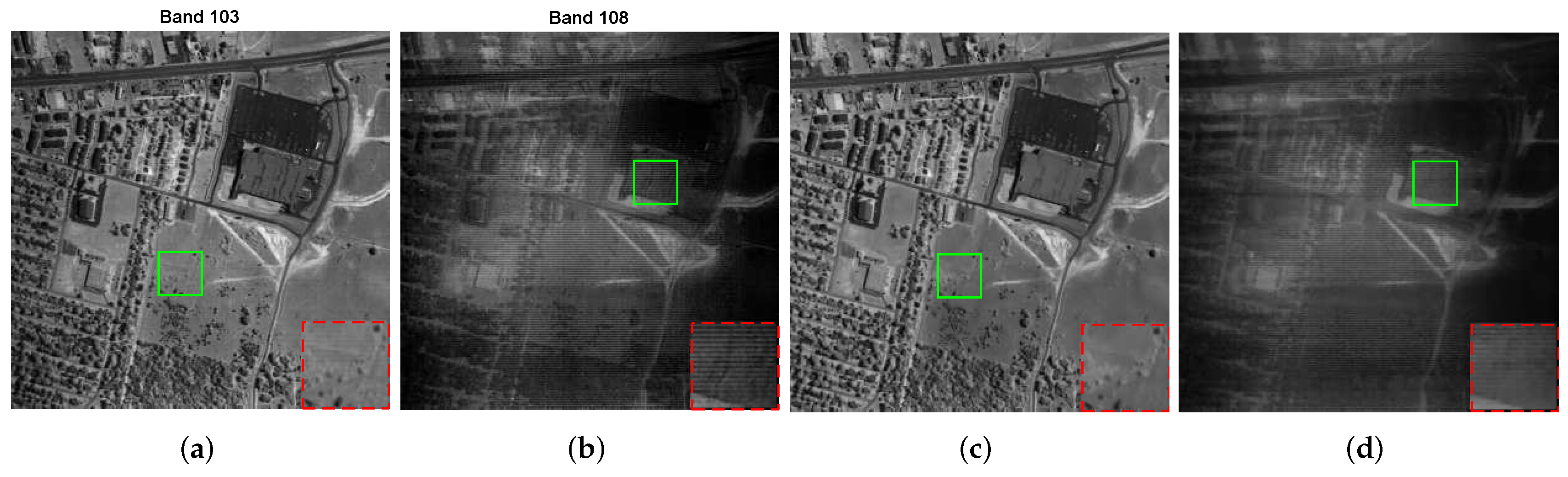
  • HYDICE Urban (Urban): This dataset was captured by the HYDICE sensor over the Copperas Cove, near Fort Hood, TX, USA, in October 1995. This scene has 307 × 307 pixels and 210 bands ranging from 0.4–2.5 μ m. The spatial resolution is 2 m/pixel and spectral resolution is 10 nm. Due to atmospheric effects and water absorption, the channels 1–4, 76, 87, 101–111, 136–153 and 198–210 are heavily corrupted. In the experiment, we employ the Urban dataset with all bands to demonstrate the superiority of SDTVLA solver for removing the most complex mixed noise. The falsecolor image of it is shown in Figure 4d.
  • AVIRIS Indian Pines (Indian Pines): This dataset was acquired by the AVIRIS instrument over the Indian Pines test site in Northwestern Indiana in 1992. This scene has 145 × 145 pixels and 220 bands. It is mainly contaminated by severe Gaussian noise, stripes, and dead lines. The falsecolor image of it is shown in Figure 4e.

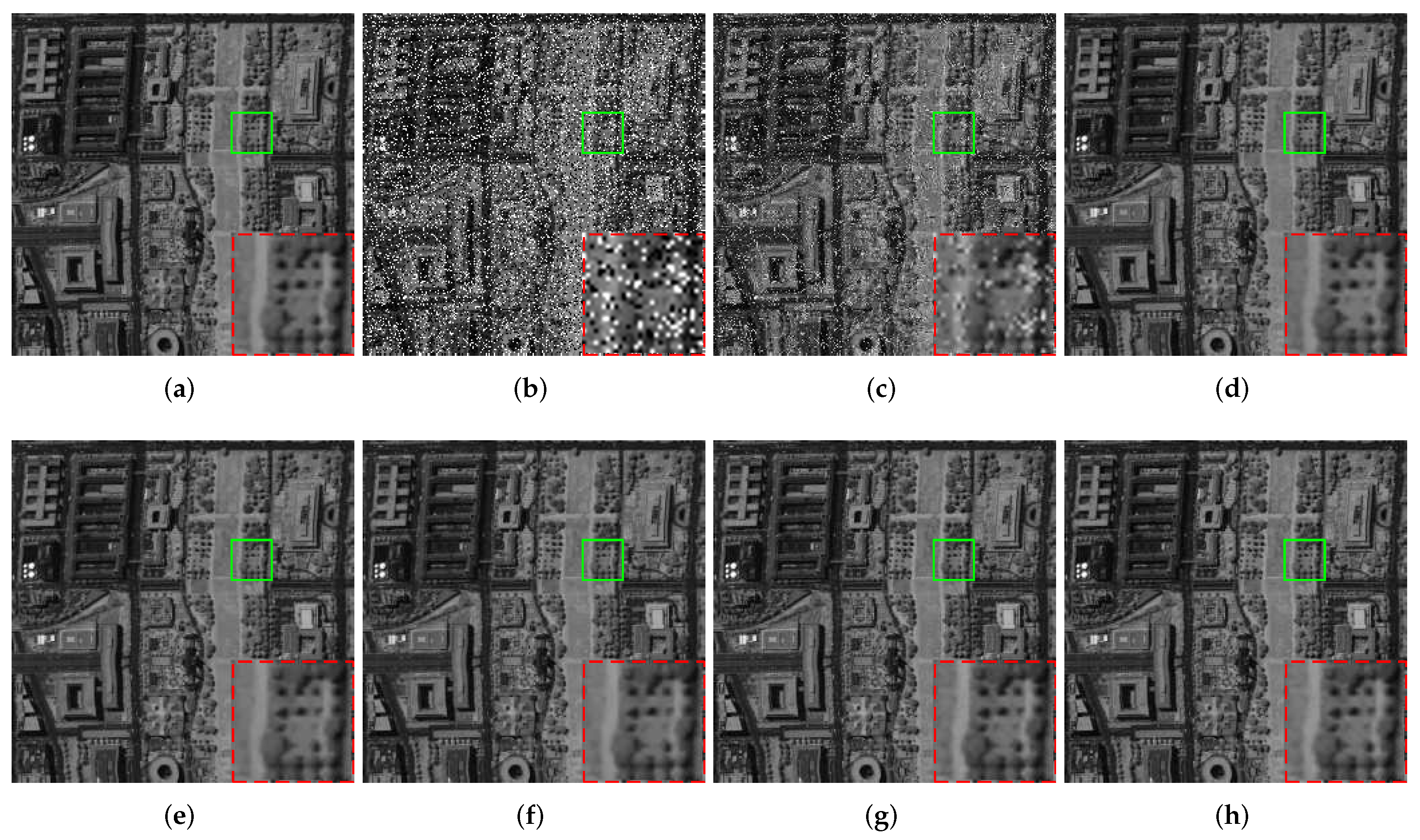
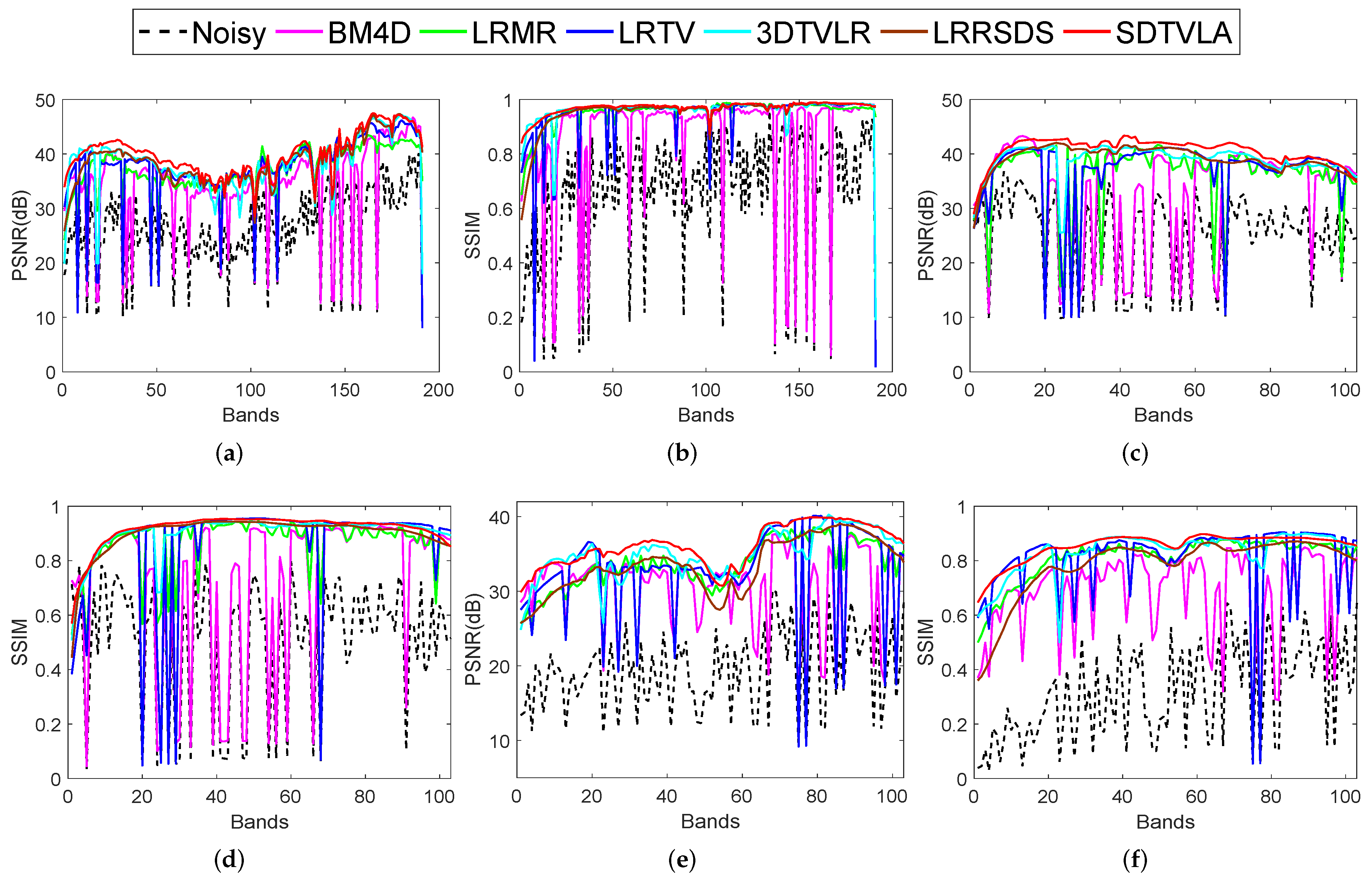
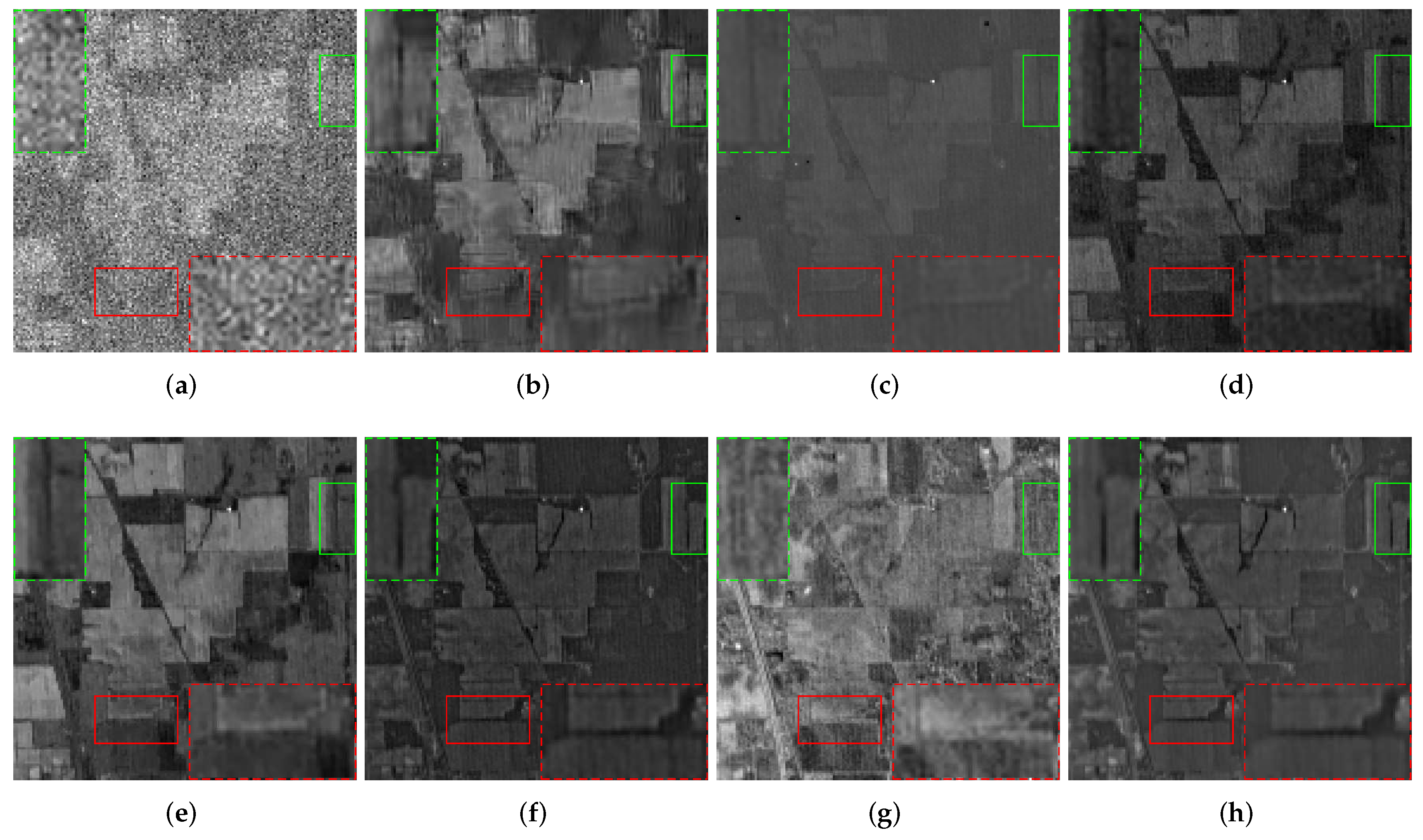
4.2. Competitive Methods and Assessment Indexes

To fully verify the superiority of the SDTVLA algorithm, the following state-of-the-art denoising methods were used to be the benchmarks.
  • BM4D [53]: one of the representative wavelet denoisers which explores the nonlocal self-similarities in a tensor manner and achieves great success in nature image denoising.
  • LRMR [34]: one of the outstanding HSI mixed denoising methods by using so-called “GoDec” algorithm to solve the patch-based low-rank matrix recovery problem.
  • LRTV [43]: a novel band-by-band TV regularized LRR method for mixed noise reduction of HSI.
  • 3DTVLR [45]: a novel mixed noise removal method combining three-dimensional TV (spatial TV and spectral TV) and LRR for HSI.
  • LRRSDS [48]: one of the state-of-the-art mixed noise reduction methods by enforcing the low-rank constraint in the SDS.
In addition, to quantitatively assess the denoising results, several evaluation indicators, such as the mean peak signal-to-noise ratio (MPSNR), the mean structural similarity (MSSIM), the mean feature similarity (MFSIM) [54], erreur relative globale adimensionelle de synthese (ERGAS) [55] and the mean spectral angle (MSA), were employed.

4.3. Experiments on Simulated Datasets

The simulation experiments are conducted in WDC, Pavia and Gulf datasets, because these three datasets all have a high image quality in each band and can be treated as clean HSIs. To accurately simulate the noises in a real HSI, several types of noises were added to each dataset according to the following criteria.
  • To generate the noisy HSI with difference noise intensity, we add zero-mean Gaussian noise to all bands. However, for each band, the noise variance is randomly generated from 0.049 to 0.098. It means the signal-to-noise-ratio (SNR) of noise lies in [10–20] dB.
  • Since the impulse noise is usually generated by the water absorption or atmosphere effect and is often present in continuous bands, we add the impulse noise to the bands from 90 to 110 with the density of 20% pixels being contaminated;
  • Caused by the sensors, dead lines or stripes always exist in the HSI. Therefore, we add dead lines to 10 bands, and the width of each dead line is randomly set from 1 to 3.
The parameters of the comparison algorithms are tuned slightly according to the default values in the corresponding literatures. In addition, the results presented in the following experiments are based on the highest value of MPSNR. For the SDTVLA solver, four parameters are set as λ 1 = 0.01 , λ 2 = 0.2 , ρ = 0.1 and r = 2 . To make the reader easy to reproduce the algorithm, Table 1 lists the optimal values of the parameters for each competitive method. Moreover, the MATLAB source code of the proposed algorithm as well as the competitive methods are released at the author’s homepage (see Supplementary Materials for details).
Figure 5 illustrates the denoising results of band 59 obtained by the competitive methods in the simulated WDC dataset. In the simulation, band 59 is corrupted by severe impulse noise and Gaussian noise simultaneously. It is clear that BM4D is not good at getting rid of the impulse noise due to lack of the sparse term modeling. All low-rank-based denoisers (e.g., LRMR, LRTV, 3DTVLR, LRRSDS and SDTVLA) can successfully get rid of both impulse noise and Gaussian noise. The difference is that the methods with local spatial constraints (e.g., LRTV, 3DTVLR, SDTVLA) can produce more precise results than their only low-rank-based counterparts (e.g., LRMR and LRRSDS). Among all competitive methods, the proposed SDTVLA delivers the best result in removing all noises and preserving the fine details in both spatial and spectral domains.
Figure 6 presents the denoising results of band 84 image for the simulated WDC dataset. This band is the mostly contaminated band in the dataset, it is simultaneously simulated with impulse noise, Gaussian noise, and the dead lines. From the illustration, it is obvious that the SDTVLA solver can perfectly get rid of all types of mixed noises and produce the best results in visual effects. Due to lack of sparse noise modeling, BM4D is almost incompetent to the impulse noise and dead lines. For the LRMR denoiser, most of the Gaussian noise and all the impulse noise are successfully removed, but some of the dead lines are still retained in the results (see the details in purple ellipse). LRTV significantly removes almost all the impulse and Gaussian noises. However, for the dead lines, LRTV cannot get rid of any of it and behaves even worse than LRMR. This phenomenon validates our analysis above, that is, when stripes or dead lines exist in the band, the TV regularizer will appear to be negative and prevent the low-rank term from getting rid of them. Because 3DTVLR method assigns the same weights for each pixel (especially for the weights of spectral TV), some dead lines are successfully removed but some dead lines are still partially retained (see the details in blue ellipse of Figure 6f). Without enforcing the spatial local correlation, LRRSDS can only get rid of the severe Gaussian noise to an extent (compare the zoomed-in portions in red rectangles of Figure 6g,h, respectively).
Figure 7 plots the spectrum of the pixel located at ( 110 , 206 ) in the simulated WDC dataset before and after restoration. It is clear that the SDTVLA solver yields the best estimate of the original spectrum. This conclusion can also be drawn from the difference spectrum in Figure 7h, and it shows that SDTVLA gives the minimum residual spectrum. For the BM4D and LRTV methods, both produce several fluctuations in the spectrum (see Figure 7c,e), indicating that these two methods cannot get rid of the stripes or dead lines completely. For the LRMR denoiser, it can remove all kinds of noises to an extent. However, there are still some small fluctuations in the restored spectrum (see the details in purple ellipse and green rectangle). For the 3DTVLR denoiser, it can produce better results than the above three denoisers in getting rid of the mixed noise for HSI. One of its main drawbacks is that it sometimes does not precisely recover the first or last few bands due to the unbalanced spectral continuity enforced by the spectral TV regularizer. For instance, as shown in the difference spectrum of Figure 7f, it is obvious that the digital number (DN) values of the first few bands deviate too much (i.e., more than 1000) from the DN values in the original spectrum. For the LRRSDS denoiser, we can observe that it does not restore the spectrum as precise as that of SDTVLA method, especially in the parts highlighted by the purple ellipse and green rectangle in Figure 7g.
To further verify the denoising performance of the SDTVLA solver on each band, Figure 8 presents the PSNR and SSIM values as a function of the bands regarding different methods in WDC, Pavia University and Gulf datasets. It leads us to conclude that the SDTVLA solver achieves higher PSNR and SSIM values than other algorithms in almost all bands. This phenomenon also makes great consistence with the visual results. In addition, it can be found that there are many serious fluctuations in the BM4D and LRTV results, especially for those bands with stripes or dead lines. It indicates that these two methods fail to remove the stripes or dead lines completely. For the LRMR method, it can also be found that there are several fluctuations in the result of Pavia University dataset. This phenomenon reveals that LRMR sometimes also produces inaccurate results due to the correlated structures in the data. For the 3DTVLR and LRRSDS methods, they can successfully remove all kinds of noises; however, the details of the data are not preserved as well as the SDTVLA method does.
Table 2 exhibits the assessment indexes of the denoising results regarding different algorithms in the three simulated datasets. It draws the similar conclusion as that from the above illustrations, that is, the proposed SDTVLA solver delivers the best assessment metric values in all terms of MPSNR, MSSIM, FSSIM, ERGAS and MSA. Specifically, the proposed SDTVLA method produces about 1.5 dB higher PSNR values and 0.01 rad lower MSA values than the second-best method (i.e., 3DTVLR or LRRSDS). In addition, the average runtime of each method for these three simulated datasets are also listed in Table 2. All algorithms are implemented by MATLAB 2017a in Windows system with Intel Core i7 3.6 GHz CUP and 8 GB RAM. Compared with 3DTVLR and LRRSDS methods, the proposed SDTVLA solver explores both local smoothness and global low rankness in SDS. Therefore, it costs more computational time than other state-of-the-art methods.
In summary, the proposed SDTVLA method can produce the best results in both visual effects and quantitative assessment. Moreover, it shows overwhelming superiority in removing the complex mixed noises as well as preserving the spatial-spectral details when compared with the other state-of-the-art denoisers.

4.4. Experiments on Real Datasets

The second experiment was conducted in Urban and Indian Pines datasets. Both scenes are seriously contaminated by the Gaussian noise, stripes, and dead lines as well as atmosphere effect and water absorption. It is worth noting that the stripes existing in Urban are strongly structured, which means that they have very strongly correlated patterns. In addition, some continuous bands (i.e., band 105 to band 150) are affected by bias illumination, see the details in Figure 9c–e.
In the experiment for the two real HSI datasets, BM4D, LRMR, LRTV, 3DTVLR and LRRSDS methods were implemented by slightly adjusting the parameters to achieve the optimal visual results according to the rules for setting the parameters in the simulated datasets. In addition, a new denoising method, i.e., 3-dimensional cross TV method (3DCrTV) [51], is added for comparison. The details of the parameters setting for the comparison methods are listed in Table 3.
Figure 9 illustrates the images of band 2, 104, 107, 141, 150, 208 and the denoising results of competitive methods. Among them, the observed image of band 2 is slightly contaminated by the Gaussian noise and stripes and band 104 is contaminated by severe Gaussian noise, impulse noise, and stripes. The observed images of band 107, 141, 150 and 208 are heavily corrupted by severe mixed noises and bias illumination. It is obvious that the SDTVLA solver delivers the optimal results than the other comparison denoisers in visual effect. It completely gets rid of the complex mixed noises and bias illumination due to its full exploration of useful structures in the SDS. BM4D behaves badly in getting rid of the impulse noise and stripes in Urban dataset (see the second row of Figure 9), because it follows the assumption that the noise is mainly Gaussian. Besides, BM4D oversmoothes the portions heavily corrupted by the Gaussian noise. LRMR and LRTV denoisers can get rid of the Gaussian noise and impulse noise completely (see the third and fourth rows in Figure 9a), but neither of them can successfully get rid of the structured stripes, for instance, many stripes are maintained in the restored results in the third and fourth rows of Figure 9b,c,e. Because the stripes existing in Urban dataset all locate at the same place from band 100 to 145. In addition, from Figure 9d,e, it clearly shows that LRMR and LRTV are not good at alleviating the impact of bias illumination. The 3DTVLR method can successfully remove most of the structured stripes by strengthening the weights of the spectral TV and get rid of the Gaussian noise and impulse noise. However, due to the severe mixed noise and bias illumination in the continuous bands, lots of details in the restored results of 3DTVLR are lost, see the fifth row of Figure 9c–e. For the 3DCrTV and LRRSDS methods, both explore the information in the SDS and can get rid of the Gaussian noise and impulse noise successfully. The difference is that 3DCrTV can successfully suppress the structured stripes (see the zoom-in portions in the sixth row of Figure 9b,c) but fail to get rid of the impact of bias illumination (see the sixth row of Figure 9e,f) by enforcing the local TV constraint, while LRRSDS is good at removing the bias illumination (see the seventh row of Figure 9e,f) but fail to remove the structured stripes completely (see the seventh row of Figure 9b,c) by exploiting the low-rank properties from the whole scene.
Figure 10 presents the horizontal mean profiles of band 109 before and after denoising by different algorithms in Urban dataset. As plotted in Figure 10a, due to the existence of stripes and dead lines, there are rapid fluctuations in the observed curve. After denoising, it can be seen that the fluctuations are more or less reduced by the competitive algorithms. However, there are still many rapid fluctuations existing in the outputs of BM4D, LRMR, LRTV and LRRSDS, because the structured stripes are treated as low-rank features by these LR-based algorithms. It also indicates that the HTV cannot successfully assist LR technique to completely remove the structured stripes or dead lines. For the 3DTVLRT denoiser, it successfully gets rid of the mixed noises, especially the stripes and dead lines. However, due to the larger weight in spectral direction, 3DTVLR devotes to enforcing the reconstructed band to be as approximate as possible to its upper and lower bands, thus losing lots of fine details in spatial-spectral domains (see the parts in blue and brown rectangles of Figure 10e). For 3DCrTV method, it fails to suppress the bias illumination at the middle of the image (see the part in blue rectangle of Figure 10f), and also loses some fine details (see the part in red ellipse of Figure 10f). For the proposed SDTVLA, it completely removes the complex mixed noises as well as the bias illumination and finally produces the best mean profile curve with more details.
To further validate the superior performance of the SDTVLA solver, two typical bands, i.e., band 107 and band 220, of the Indian Pine dataset are illustrated in Figure 11 and Figure 12 to show the performance of all competitive algorithms. Here, it leads us to draw the same conclusion that the SDTVLA solver still gets the best performance for removing the complex mixed noises. Moreover, from the zoom-in portions within the red and green rectangles, SDTVLA preserves more fine details than other comparison denoisers. For the BM4D denoiser, it still fails to remove the impulse noise and stripes. For the LRMR denoiser, there are still lots of Gaussian noise left in the results. For TVLR and 3DTVLR, they distort many fine details by exploring the spatial smoothness with improper strength. For 3DCrTV and LRRSDS, they cannot reconstruct the images with more fine details as SDTVLA does due to lack of the combination of global and local priors.

4.5. Discussion

Basically, we introduced a new spectral difference-induced TV and low-rank approximation method for mixed denoising of HSI. Different from the existing low-rank-based methods, our method mainly exploits the useful information in the SDS. First, spectral difference projection can effectively change the intrinsic structures of the noises, especially for the structured stripes and dead lines, so that LR technique can successfully get rid of them. Besides, the total variation in SDS can be treated as a local correlation of the residual HSI and it is much sparser than the TV in original HSI. Moreover, low rankness can be treated as one of the intrinsic properties of the whole HSI data. Therefore, the proposed SDTVLA simultaneously explores the local piecewise correlation and global low rankness of HSI cube in the SDS.
In the SDTVLA model, there are totally four parameters that need to be carefully identified. In the following, we will analyze the impact of each parameter on the restoration results of the SDTVLA algorithm. Specifically, a systematical discussion on how to choose such parameters in our experiments will be addressed. All the results are based on the simulated experiment in WDC dataset.
(1) The impact of parameters λ 1 and λ 2 . The two parameters are related to the density of sparse noise (i.e., impulse noise, stripes, and dead lines) and TV regularized low-rank regularizer, respectively. Figure 13a,b plot the MPSNR and MSSIM values as a function of λ 1 and λ 2 for the proposed SDTVLA solver in WDC dataset, where λ 1 is chosen from the set { 0.001 , 0.01 , 0.02 , 0.03 , 0.04 , 0.05 , 0.06 } and λ 2 is chosen from the set { 0.01 , 0.05 , 0.1 , 0.2 , 0.25 , 0.3 , 0.35 , 0.4 , 0.45 } . It is obvious that the SDTVLA solver is quite robust to these two parameters. When λ 1 lies in the range of [0.01–0.06] and λ 2 lies in the range of [0.01–0.45], SDTVLA can produce an appealing result.
(2) The impact of the desired rank r. In the optimization of SDTVLA, we use the nuclear norm to encode the low-rank prior. Under the linear mixture model of HSI, as analyzed in LRMR solver, the value of r should be equivalent to the exact number of endmembers in the HSI. However, in SDTVLA model, we exploited the low-rank property in the SDS. According to | | L X | | * | | X | | * (here, L is a linear transformation), the value of r in SDTVLA solver should be smaller or equal to the number of endmembers. Figure 13c,d plot the MPSNR and MSSIM values as a function of λ 1 and r, respectively. From it, we can see that the parameter r indeed has a strong impact on the result. However, when r lies in the range of [1–4], SDTVLA can produce an optimal result.
(3) The impact of the spectral proportion ρ . The parameter ρ plays an important role to keep the balance of the TV regularization and low-rank constraint. Figure 13e,f plot the MPSNR and MSSIM values as a function of the parameter ρ . It clearly shows the benefit of tuning such a parameter.
(4) The convergence of SDTVLA solver.Figure 14 presents the MPSNR and MSSIM gains as a function of the iteration number of the SDTVLA solver. It is clear to see that the MPSNR and MSSIM values rapidly converge to the stable values as the number of iteration increases. This phenomenon proves convergence of the SDTVLA solver.

5. Conclusions

In this paper, we proposed a new HSI mixed denoising method by combining the TV regularization and low-rank approximation in the SDS. Specifically, the low-rank approximation in SDS is employed to explore the global spectral correlation from all bands and a TV in SDS regularizer is adopted to describe the piecewise smoothness in spatial-spectral domains of HSI. Therefore, the proposed SDTVLA method thoroughly exploits both spectrally global low rankness and spatially local smoothness in the spectral difference space. It discloses the fact that TVLA term in SDS could significantly get rid of the complex mixed noise. Extensive experiments on three simulated HSI datasets and two real HSI datasets validate the overwhelming superiority of the proposed SDTVLA solver over other comparison denoisers in removing the severely mixed noises, especially for the heavy Gaussian noise and structured sparse noise. Specifically, from the results of simulated experiments, we can easily observe that the MPSNR values achieved by the proposed SDTVLA are about 1.5 dB higher than those of the second-best denoiser. For the experiment in real Urban dataset, the proposed SDTVLA shows the overwhelming advantages in removing the complex mixed noises and the bias illumination.
Next, we are planning to incorporate the noise-adjusting modeling into our SDTVLA solver to further improve its capability of dealing with more complex noises. Meanwhile, we will also consider implementing the proposed algorithm on a GPU or cloud platform to reduce runtime for more real-time applications.

Supplementary Materials

The source code of the proposed method as well as the competitive methods are available from the author’s homepage: http://www.escience.cn/people/LeSun/index.html.

Author Contributions

L.S. wrote the manuscript; L.S. and T.Z. conceived and designed the experiments; L.S. performed the experiments and analyzed the results; L.S. and Z.W. analyzed the data; L.X. and B.J. revised the paper.

Funding

This study was funded by the National Natural Science Foundation of China and Jiangsu Province [Grant No. 61601236, BK20150923, 61502206, 61571230] and the PAPD fund (a project funded by the priority academic program development of Jiangsu Higher Education Institutions).

Acknowledgments

We thank the three anonymous reviewers and academic editor for their comments and suggestions.

Conflicts of Interest

The authors declare no conflict of interest.

References

  1. Bioucas-Dias, J.M.; Plaza, A.; Camps-Valls, G.; Scheunders, P.; Nasrabadi, N.; Chanussot, J. Hyperspectral remote sensing data analysis and future challenges. IEEE Geosci. Remote Sens. Mag. 2013, 1, 6–36. [Google Scholar] [CrossRef]
  2. Sun, L.; Wu, Z.; Liu, J.; Xiao, L.; Wei, Z. Supervised spectral–spatial hyperspectral image classification with weighted Markov random fields. IEEE Trans. Geosci. Remote Sens. 2015, 53, 1490–1503. [Google Scholar] [CrossRef]
  3. Sun, L.; Wang, S.; Wang, J.; Zheng, Y.; Jeon, B. Hyperspectral classification employing spatial-spectral low rank representation in hidden fields. J. Ambient Intell. Humaniz. Comput. 2017, 1–12. [Google Scholar] [CrossRef]
  4. Wu, Z.; Shi, L.; Li, J.; Wang, Q.; Sun, L.; Wei, Z.; Plaza, J.; Plaza, A. GPU parallel implementation of spatially adaptive hyperspectral image classification. IEEE J. Sel. Top. Appl. Earth Obs. Remote Sens. 2018, 11, 1131–1143. [Google Scholar] [CrossRef]
  5. Zhang, L.; Zhao, C. A spectral-spatial method based on low-rank and sparse matrix decomposition for hyperspectral anomaly detection. Int. J. Remote Sens. 2017, 38, 4047–4068. [Google Scholar] [CrossRef]
  6. Sun, L.; Wu, Z.; Xiao, L.; Liu, J.; Wei, Z.; Dang, F. A novel l 1/2 sparse regression method for hyperspectral unmixing. Int. J. Remote Sens. 2013, 34, 6983–7001. [Google Scholar] [CrossRef]
  7. Sun, L.; Ge, W.; Chen, Y.; Zhang, J.; Jeon, B. Hyperspectral unmixing employing l1-l2 sparsity and total variation regularization. Int. J. Remote Sens. 2018, 39, 6037–6060. [Google Scholar] [CrossRef]
  8. Lee, J.B.; Woodyatt, A.S.; Berman, M. Enhancement of high spectral resolution remote-sensing data by a noise-adjusted principal components transform. IEEE Trans. Geosci. Remote Sens. 1990, 28, 295–304. [Google Scholar] [CrossRef]
  9. Green, A.A.; Berman, M.; Switzer, P.; Craig, M.D. A transformation for ordering multispectral data in terms of image quality with implications for noise removal. IEEE Trans. Geosci. Remote Sens. 1988, 26, 65–74. [Google Scholar] [CrossRef] [Green Version]
  10. Zhang, M.; Gunturk, B.K. Multiresolution bilateral filtering for image denoising. IEEE Trans. Image Process. 2008, 17, 2324–2333. [Google Scholar] [CrossRef]
  11. Vese, L.A.; Osher, S.J. Image denoising and decomposition with total variation minimization and oscillatory functions. J. Math. Imaging Vis. 2004, 20, 7–18. [Google Scholar] [CrossRef]
  12. Buades, A.; Coll, B.; Morel, J.M. A non-local algorithm for image denoising. In Proceedings of the IEEE Computer Society Conference on Computer Vision and Pattern Recognition, Boston, MA, USA, 7–12 June 2005; Volume 2, pp. 60–65. [Google Scholar]
  13. Jain, V.; Seung, S. Natural image denoising with convolutional networks. In Proceedings of the Advances in Neural Information Processing Systems, Vancouver, BC, Canada, 7–10 December 2009; pp. 769–776. [Google Scholar]
  14. Tang, Z.; Ling, M.; Yao, H.; Qian, Z.; Zhang, X.; Zhang, J.; Xu, S. Robust image hashing via random Gabor filtering and DWT. Comput. Mater. Contin. 2018, 55, 331–344. [Google Scholar]
  15. Rasti, B.; Sveinsson, J.R.; Ulfarsson, M.O.; Benediktsson, J.A. Hyperspectral image denoising using 3D wavelets. In Proceedings of the IEEE International Conference on Geoscience and Remote Sensing Symposium (IGARSS 2012), Munich, Germany, 22–27 July 2012; pp. 1349–1352. [Google Scholar]
  16. Zelinski, A.; Goyal, V. Denoising hyperspectral imagery and recovering junk bands using wavelets and sparse approximation. In Proceedings of the IEEE International Conference on Geoscience and Remote Sensing Symposium, Denver, CO, USA, 31 July–4 August 2006; pp. 387–390. [Google Scholar]
  17. Chen, G.; Qian, S.E. Denoising of hyperspectral imagery using principal component analysis and wavelet shrinkage. IEEE Trans. Geosci. Remote Sens. 2011, 49, 973–980. [Google Scholar] [CrossRef]
  18. Chen, G.; Bui, T.D.; Quach, K.G.; Qian, S.E. Denoising hyperspectral imagery using principal component analysis and block-matching 4D filtering. Can. J. Remote Sens. 2014, 40, 60–66. [Google Scholar] [CrossRef]
  19. Rasti, B.; Sveinsson, J.R.; Ulfarsson, M.O. Wavelet-based sparse reduced-rank regression for hyperspectral image restoration. IEEE Trans. Geosci. Remote Sens. 2014, 52, 6688–6698. [Google Scholar] [CrossRef]
  20. Rasti, B.; Ulfarsson, M.O.; Ghamisi, P. Automatic hyperspectral image restoration using sparse and low-rank modeling. IEEE Geosci. Remote Sens. Lett. 2017, 14, 2335–2339. [Google Scholar] [CrossRef]
  21. Wang, R.; Shen, M.; Li, Y.; Gomes, S. Multi-task joint sparse representation classification based on fisher discrimination dictionary learning. Comput. Mater. Contin. 2018, 57, 25–48. [Google Scholar] [CrossRef]
  22. Zhao, Y.Q.; Yang, J. Hyperspectral image denoising via sparse representation and low-rank constraint. IEEE Trans. Geosci. Remote Sens. 2015, 53, 296–308. [Google Scholar] [CrossRef]
  23. Li, J.; Yuan, Q.; Shen, H.; Zhang, L. Noise removal from hyperspectral image with joint spectral-spatial distributed sparse representation. IEEE Trans. Geosci. Remote Sens. 2016, 54, 5425–5439. [Google Scholar] [CrossRef]
  24. Lu, T.; Li, S.; Fang, L.; Ma, Y.; Benediktsson, J.A. Spectral–spatial adaptive sparse representation for hyperspectral image denoising. IEEE Trans. Geosci. Remote Sens. 2016, 54, 373–385. [Google Scholar] [CrossRef]
  25. Fu, Y.; Lam, A.; Sato, I.; Sato, Y. Adaptive spatial-spectral dictionary learning for hyperspectral image restoration. Int. J. Comput. Vis. 2017, 122, 228–245. [Google Scholar] [CrossRef]
  26. Zhuang, L.; Bioucas-Dias, J.M. Fast hyperspectral image denoising and inpainting based on low-rank and sparse representations. IEEE J. Sel. Top. Appl. Earth Obs. Remote Sens. 2018, 11, 730–742. [Google Scholar] [CrossRef]
  27. Rasti, B.; Scheunders, P.; Ghamisi, P.; Licciardi, G.; Chanussot, J. Noise reduction in hyperspectral imagery: Overview and application. Remote Sens. 2018, 10, 482. [Google Scholar] [CrossRef]
  28. Fang, W.; Zhang, F.; Sheng, V.S.; Ding, Y. A method for improving CNN-based image recognition using DCGAN. Comput. Mater. Contin. 2018, 57, 167–178. [Google Scholar] [CrossRef]
  29. Zhang, Y.; Wang, Q.; Li, Y.; Wu, X. Sentiment classification based on piecewise pooling convolutional neural network. Comput. Mater. Contin. 2018, 56, 285–297. [Google Scholar]
  30. Meng, R.; Rice, S.G.; Wang, J.; Sun, X. A fusion steganographic algorithm based on faster R-CNN. Comput. Mater. Contin. 2018, 55, 1–16. [Google Scholar]
  31. Li, Y.; Xie, W.; Li, H. Hyperspectral image reconstruction by deep convolutional neural network for classification. Pattern Recognit. 2017, 63, 371–383. [Google Scholar] [CrossRef]
  32. Xie, W.; Li, Y. Hyperspectral imagery denoising by deep learning with trainable nonlinearity function. IEEE Geosci. Remote Sens. Lett. 2017, 14, 1963–1967. [Google Scholar] [CrossRef]
  33. Lu, X.; Wang, Y.; Yuan, Y. Graph-regularized low-rank representation for destriping of hyperspectral images. IEEE Trans. Geosci. Remote Sens. 2013, 51, 4009–4018. [Google Scholar] [CrossRef]
  34. Zhang, H.; He, W.; Zhang, L.; Shen, H.; Yuan, Q. Hyperspectral image restoration using low-rank matrix recovery. IEEE Trans. Geosci. Remote Sens. 2014, 52, 4729–4743. [Google Scholar] [CrossRef]
  35. Zhou, T.; Tao, D. Godec: Randomized low-rank & sparse matrix decomposition in noisy case. In Proceedings of the International Conference on Machine Learning, Bellevue, WA, USA, 28 June–2 July 2011; pp. 1–8. [Google Scholar]
  36. Zhu, R.; Dong, M.; Xue, J.H. Spectral nonlocal restoration of hyperspectral images with low-rank property. IEEE J. Sel. Top. Appl. Earth Obs. Remote Sens. 2015, 8, 3062–3067. [Google Scholar]
  37. Wang, M.; Yu, J.; Xue, J.H.; Sun, W. Denoising of hyperspectral images using group low-rank representation. IEEE J. Sel. Top. Appl. Earth Obs. Remote Sens. 2016, 9, 4420–4427. [Google Scholar] [CrossRef]
  38. He, W.; Zhang, H.; Zhang, L.; Shen, H. Hyperspectral image denoising via noise-adjusted iterative low-rank matrix approximation. IEEE J. Sel. Top. Appl. Earth Obs. Remote Sens. 2015, 8, 3050–3061. [Google Scholar] [CrossRef]
  39. Sun, L.; Jeon, B.; Soomro, B.N.; Zheng, Y.; Wu, Z.; Xiao, L. Fast superpixel based subspace low rank learning method for hyperspectral denoising. IEEE Access 2018, 6, 12031–12043. [Google Scholar] [CrossRef]
  40. Fan, H.; Chen, Y.; Guo, Y.; Zhang, H.; Kuang, G. Hyperspectral image restoration using low-rank tensor recovery. IEEE J. Sel. Top. Appl. Earth Obs. Remote Sens. 2017, 10, 4589–4604. [Google Scholar] [CrossRef]
  41. Chang, Y.; Yan, L.; Fang, H.; Zhong, S.; Zhang, Z. Weighted low-rank tensor recovery for hyperspectral image restoration. arXiv, 2017; arXiv:1709.00192v1. [Google Scholar]
  42. Huang, Z.; Li, S.; Fang, L.; Li, H.; Atli, B.J. Hyperspectral image denoising with group sparse and low-rank tensor decomposition. IEEE Access 2018, 6, 1380–1390. [Google Scholar] [CrossRef]
  43. He, W.; Zhang, H.; Zhang, L.; Shen, H. Total-variation-regularized low-rank matrix factorization for hyperspectral image restoration. IEEE Trans. Geosci. Remote Sens. 2016, 54, 178–188. [Google Scholar] [CrossRef]
  44. Sun, L.; Zheng, Y.; Jeon, B. Hyperspectral restoration employing low rank and 3D total variation regularization. In Proceedings of the International Conference on Progress in Informatics and Computing (PIC), Shanghai, China, 23–25 December 2016; pp. 326–329. [Google Scholar]
  45. Sun, L.; Zhan, T.; Wu, Z.; Jeon, B. A novel 3d anisotropic total variation regularized low rank method for hyperspectral image mixed denoising. ISPRS Int. J. Geo-inf. 2018, 7, 412. [Google Scholar] [CrossRef]
  46. Wu, Z.; Wang, Q.; Jin, J.; Shen, Y. Structure tensor total variation-regularized weighted nuclear norm minimization for hyperspectral image mixed denoising. Signal Process. 2017, 131, 202–219. [Google Scholar] [CrossRef]
  47. Wang, Y.; Peng, J.; Zhao, Q.; Leung, Y.; Zhao, X.L.; Meng, D. Hyperspectral image restoration via total variation regularized low-rank tensor decomposition. IEEE J. Sel. Top. Appl. Earth Obs. Remote Sens. 2018, 11, 1227–1243. [Google Scholar] [CrossRef]
  48. Sun, L.; Jeon, B.; Zheng, Y.; Wu, Z. Hyperspectral image restoration using low-rank representation on spectral difference image. IEEE Geosci. Remote Sens. Lett. 2017, 14, 1151–1155. [Google Scholar] [CrossRef]
  49. Sun, L.; Jeon, B.; Zheng, Y. Hyperspectral restoration based on total variation regularized low rank decomposition in spectral difference space. In Proceedings of the IEEE International Workshop on Advanced Image Technology (IWAIT), Chiang Mai, Thailand, 7–9 January 2018; pp. 1–4. [Google Scholar]
  50. Lin, Z.; Chen, M.; Ma, Y. The augmented lagrange multiplier method for exact recovery of corrupted low-rank matrices. arXiv, 2010; arXiv:1009.5055. [Google Scholar]
  51. Sun, L.; Jeon, B.; Zheng, Y.; Wu, Z. A novel weighted cross total variation method for hyperspectral image mixed denoising. IEEE Access 2017, 5, 27172–27188. [Google Scholar] [CrossRef]
  52. Eckstein, J.; Yao, W. Understanding the convergence of the alternating direction method of multipliers: Theoretical and computational perspectives. Pac. J. Optim. 2015, 11, 619–644. [Google Scholar]
  53. Maggioni, M.; Katkovnik, V.; Egiazarian, K.; Foi, A. Nonlocal transform-domain filter for volumetric data denoising and reconstruction. IEEE Trans. Image Process. 2013, 22, 119–133. [Google Scholar] [CrossRef]
  54. Zhang, L.; Zhang, L.; Mou, X.; Zhang, D. FSIM: A feature similarity index for image quality assessment. IEEE Trans. Image Process. 2011, 20, 2378–2386. [Google Scholar] [CrossRef]
  55. Wald, L. Quality of high resolution synthesised images: Is there a simple criterion? In Proceedings of the International Conference on Fusion of Earth Data: Merging Point Measurements, Raster Maps and Remotely Sensed Images, SEE/URISCA, Nice, France, 11–14 January 2000; 99–103. [Google Scholar]
Figure 1. Flowchart of the proposed method.
Remotesensing 10 01956 g001
Figure 2. Images of band 103 and 108 of the restoration results in Urban dataset. (a,b) LRMR; (c,d) LRTV. (Zoom in to see the details clearly.)
Remotesensing 10 01956 g002
Figure 3. Comparison of low rankness and total variation properties in the original HSI and SDS.
Remotesensing 10 01956 g003
Figure 4. Falsecolor images of the three simulated and two real HSI datasets. (a) WDC; (b) Pavia; (c) Gulf; (d) Urban; (e) Indian Pines.
Remotesensing 10 01956 g004
Figure 5. Restoration results of band 59 for WDC dataset (the red box illustrates the zoom-in portion in the blue box). (a) Noisy-free image; (b) noisy image (PSNR = 11.94 dB); (c) BM4D (PSNR = 17.55 dB); (d) LRMR (PSNR = 34.40 dB); (e) LRTV (PSNR = 35.51 dB); (f) 3DTVLR (PSNR = 36.52 dB); (g) LRRSDS (PSNR = 33.97 dB); (h) SDTVLA (PSNR = 37.67 dB).
Remotesensing 10 01956 g005
Figure 6. Restoration results of band 84 for WDC dataset (the red box illustrates the zoom-in portion in the blue box). (a) Noisy-free image; (b) noisy image (PSNR = 16.99 dB); (c) BM4D (PSNR = 17.75 dB); (d) LRMR (PSNR = 29.04 dB); (e) LRTV (PSNR = 18.92 dB); (f) 3DTVLR (PSNR = 33.61 dB); (g) LRRSDS (PSNR = 35.03 dB); (h) SDTVLA (PSNR = 35.86 dB).
Remotesensing 10 01956 g006
Figure 7. Reconstructed spectrum of the pixel at the location of ( 110 , 206 ) in the simulated WDC dataset. (a) Noisy-free spectrum; (b) noisy spectrum; (c) BM4D; (d) LRMR; (e) LRTV; (f) 3DTVLR; (g) LRRSDS; (h) SDTVLA.
Remotesensing 10 01956 g007
Figure 8. PSNR and SSIM values as a function of the band for the simulated datasets. (a,b) WDC dataset; (c,d) Pavia University dataset; (e,f) Gulf dataset.
Remotesensing 10 01956 g008
Figure 9. Denoising results of the competitive methods in Urban dataset (Zoom in to see the details clearly).
Remotesensing 10 01956 g009
Figure 10. Horizontal mean profiles of band 109 by different algorithms in Urban dataset. (a) The observed; (b) BM4D; (c) LRMR; (d) LRTV; (e) 3DTVLR; (f) 3DCrTV; (g) LRRSDS; (h) SDTVLA.
Remotesensing 10 01956 g010
Figure 11. Restored results of band 107 by different algorithms in Indian Pines dataset. (a) The observed; (b) BM4D; (c) LRMR; (d) LRTV; (e) 3DTVLR; (f) 3DCrTV; (g) LRRSDS; (h) SDTVLA.
Remotesensing 10 01956 g011
Figure 12. Restored results of band 220 by different algorithms in Indian Pines dataset. (a) The observed; (b) BM4D; (c) LRMR; (d) LRTV; (e) 3DTVLR; (f) 3DCrTV; (g) LRRSDS; (h) SDTVLA.
Remotesensing 10 01956 g012
Figure 13. MPSNR and MSSIM as a function of the parameters (i.e., λ 1 , λ 2 , desired rank r and spectral proportion ρ ) in the proposed method for WDC dataset. (a) MPSNR VS λ 1 and λ 2 ; (b) MSSIM VS λ 1 and λ 2 ; (c) MPSNR VS r and λ 1 ; (d) MSSIM VS r and λ 1 ; (e) MPSNR VS ρ ; (f) MSSIM VS ρ .
Remotesensing 10 01956 g013
Figure 14. MPSNR and MSSIM as a function of iteration for the proposed method with WDC dataset. (a) MPSNR VS iteration; (b) MSSIM VS iteration.
Remotesensing 10 01956 g014
Table 1. Optimal parameters of the comparison algorithms on the simulated HSI datasets.
MethodsWDCPaviaGulf
BM4D [53]---
LRMR [34] q = 26 , r = 4 , k c a r d = 6000 q = 26 , r = 9 , k c a r d = 4000 q = 26 , r = 4 , k c a r d = 6000
LRTV [43] r = 8 , λ = 10 m × n , τ = 0.004 r = 8 , λ = 10 m × n , τ = 0.003 r = 6 , λ = 10 m × n , τ = 0.003
3DTVLR [45] r = 12 , λ = 10 m × n , τ = 0.003 , ρ = 7 r = 10 , λ = 10 m × n , τ = 0.004 , ρ = 7 r = 8 , λ = 10 m × n , τ = 0.003 , ρ = 7
LRRSDS [48] r = 2 , λ 1 = 0.01 , λ 2 = 0.1 r = 1 , λ 1 = 0.02 , λ 2 = 0.1 r = 1 , λ 1 = 0.05 , λ 2 = 0.1
SDTVLA r = 4 , λ 1 = 0.02 , λ 2 = 0.3 , ρ = 0.05 r = 4 , λ 1 = 0.02 , λ 2 = 0.3 , ρ = 0.05 r = 2 , λ 1 = 0.02 , λ 2 = 0.3 , ρ = 0.09
Table 2. Assessment metrics for different denoising methods in the simulated datasets (The optimal results are shown in bold and the suboptimal results are underlined).
DatasetsMetricsNoisyBM4D [53]LRMR [34]LRTV [43]3DTVLR [45]LRRSDS [48]SDTVLA
WDCMPSNR(dB)26.1334.1437.4037.6038.4338.7640.10
MSSIM0.69570.88180.96990.95750.97230.97160.9819
FSSIM0.85260.93880.98010.97270.98370.98520.9894
ERGAS404.01307.3456.39211.0581.6148.1940.58
MSA0.44340.29980.06930.14730.08960.06600.0534
PaviaMPSNR(dB)25.1132.2636.0936.8638.9439.1340.57
MSSIM0.59280.78310.93000.91250.96200.96140.9693
FSSIM0.80820.89210.96800.95460.98170.98520.9877
ERGAS556.77410.97204.60297.8955.7748.8840.78
MSA0.57110.42540.10120.27250.06970.07150.0584
GulfMPSNR(dB)19.4530.4533.6532.8735.0833.5436.12
MSSIM0.36830.81270.90710.90050.93130.88120.9399
FSSIM0.64880.90470.94970.94570.96600.94370.9689
ERGAS365.70155.6353.18177.2746.4255.3939.44
MSA0.29550.09690.03800.09790.03650.04160.0259
Runtime (s)--974.9839.9762.9712.9786.61017.1
Table 3. Parameters setting of competitive algorithms for the real HSI datasets.
MethodsUrbanIndian Pines
BM4D [53]--
LRMR [34] q = 20 , r = 7 , k c a r d = 4000 q = 20 , r = 4 , k c a r d = 4000
LRTV [43] r = 3 , λ = 10 m × n , τ = 0.001 r = 4 , λ = 10 m × n , τ = 0.0005
3DTVLR [45] r = 4 , λ = 10 m × n , τ = 0.004 , ρ = 0.5 r = 4 , λ = 10 m × n , τ = 0.004 , ρ = 0.5
3DCrTV [51] λ 1 = 0.05 , λ 2 = 0.1 , μ = 0.8 λ 1 = 0.05 , λ 2 = 0.1 , μ = 0.8
LRRSDS [48] r = 2 , λ 1 = 0.01 , λ 2 = 0.1 r = 1 , λ 1 = 0.01 , λ 2 = 0.1
SDTVLA r = 2 , λ 1 = 0.01 , λ 2 = 0.2 , ρ = 0.5 r = 2 , λ 1 = 0.01 , λ 2 = 0.2 , ρ = 0.5

