Multi-Temporal Vineyard Monitoring through UAV-Based RGB Imagery

 ,
,  ,
,  ,
,  ,
,  and
and
Abstract

1. Introduction
2. Materials and Methods
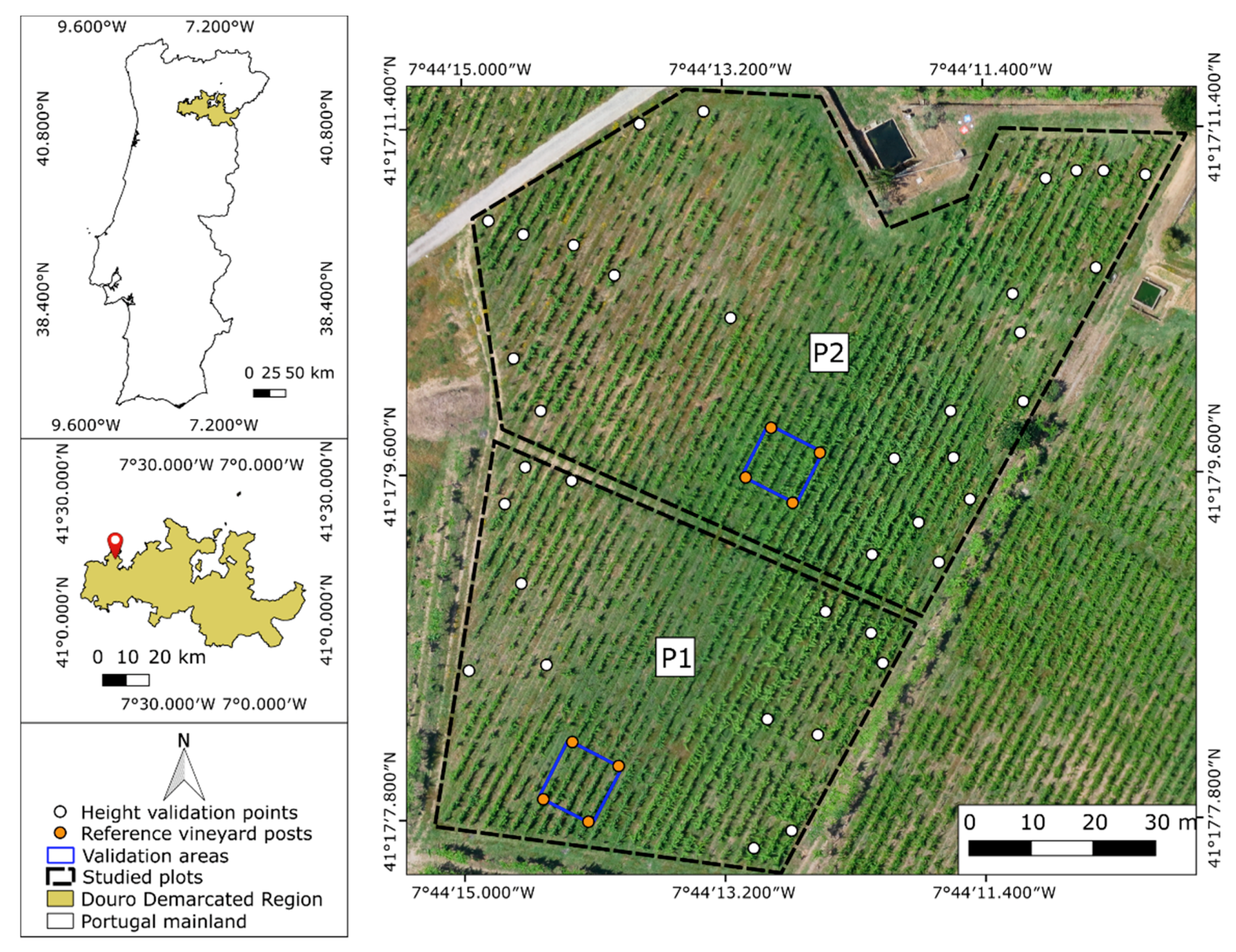
2.1. Study Area Context and Description
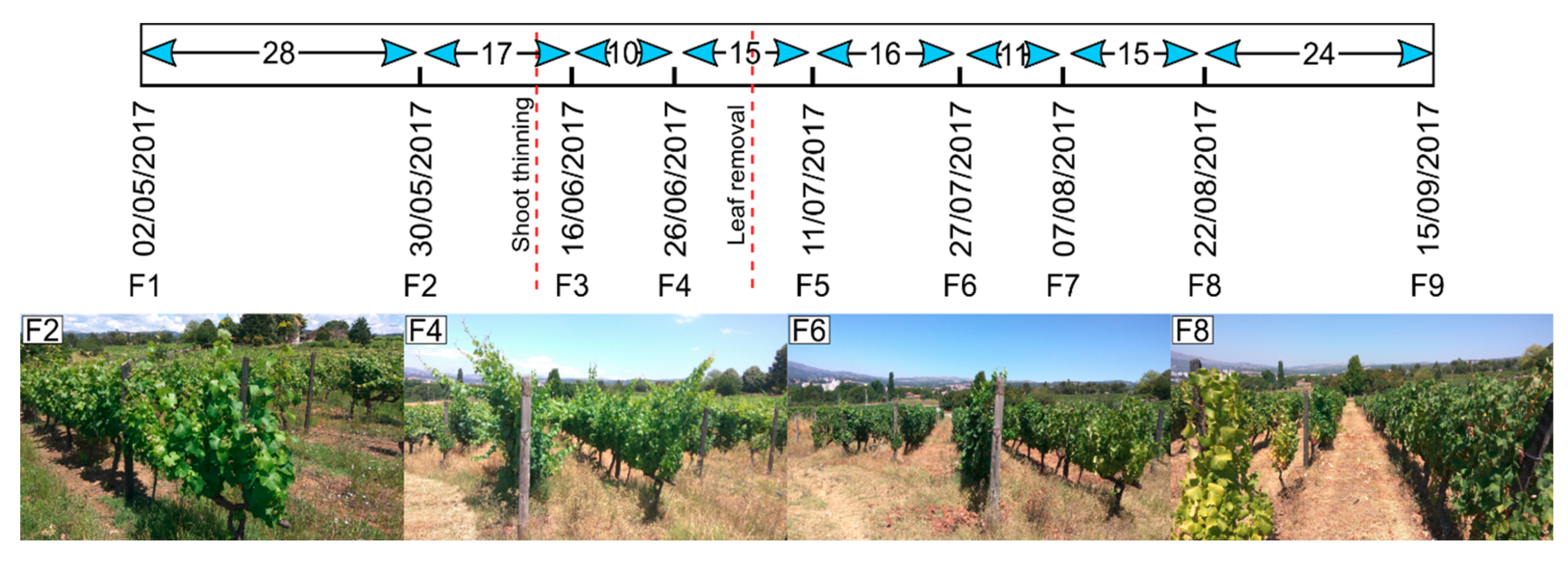
2.2. Flight Campaigns
2.3. Data Processing
2.3.1. Photogrammetric Processing
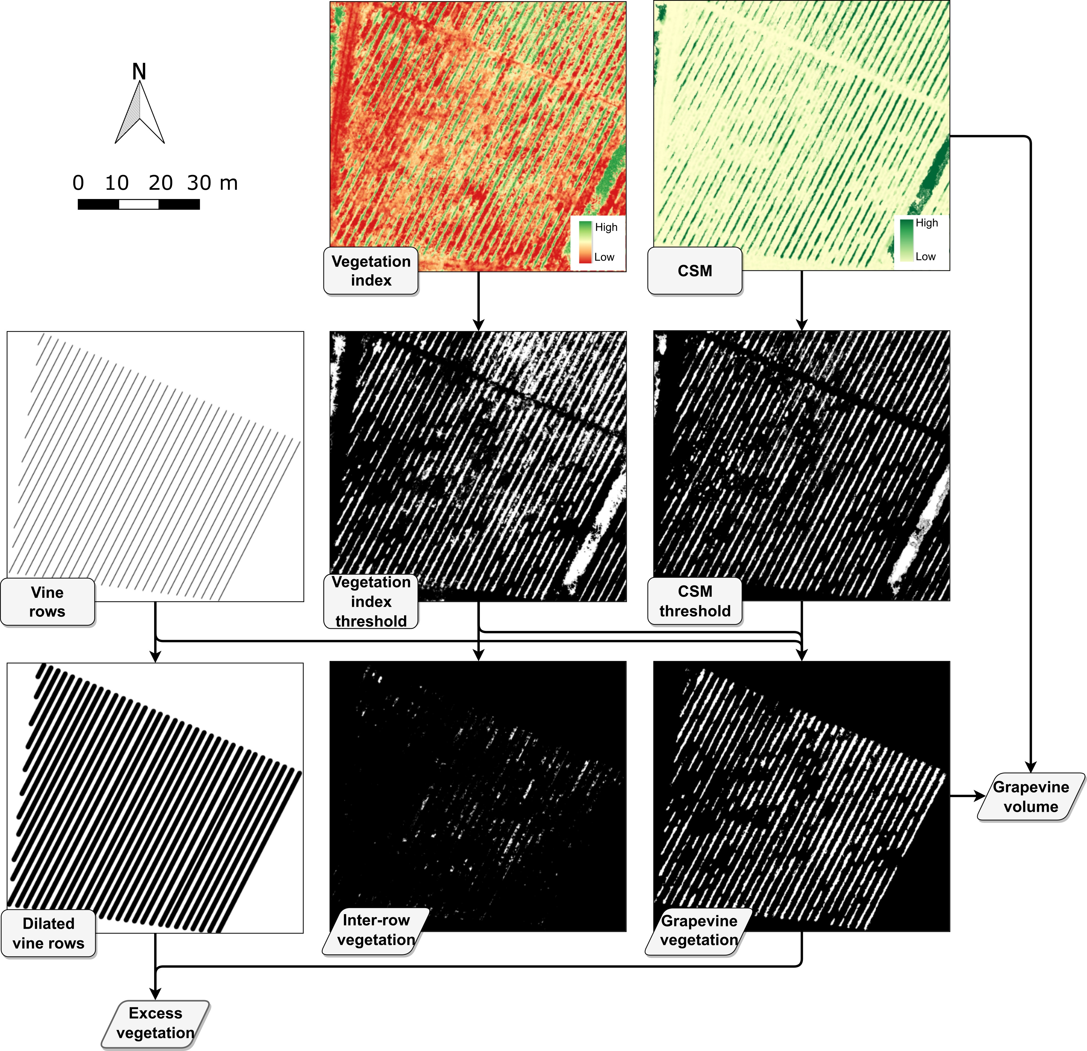
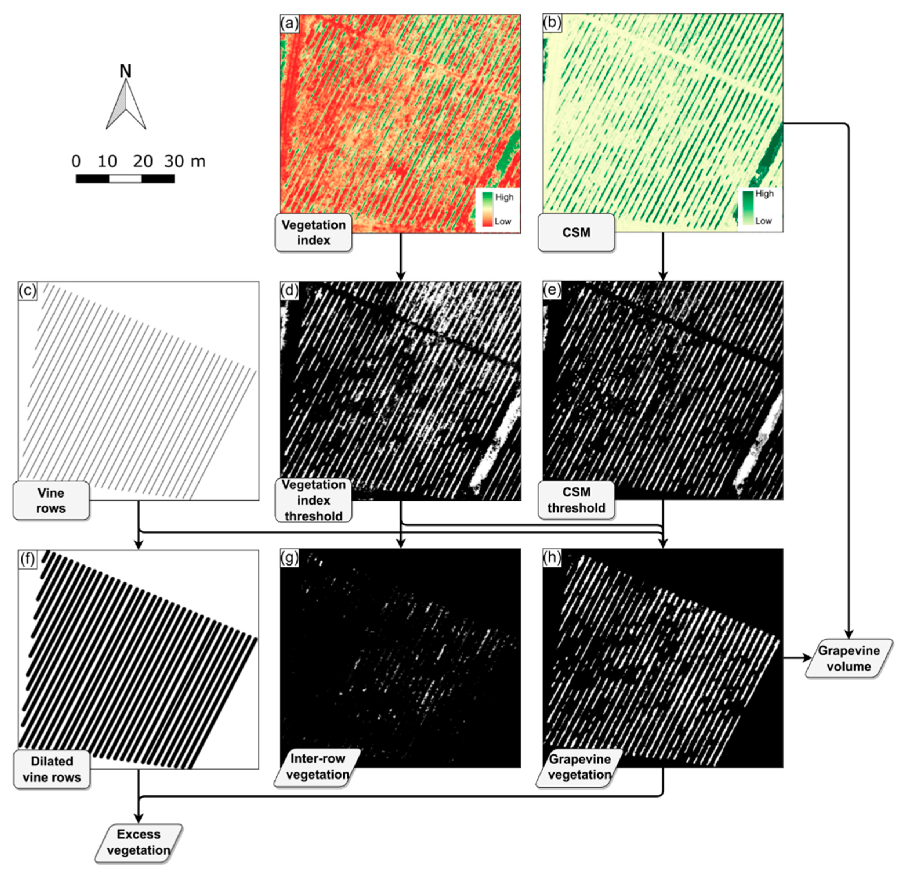
2.3.2. Vineyard Properties Extraction
2.3.3. Multi-Temporal Analysis Procedure
2.3.4. Canopy Management
2.3.5. Validation Procedure
3. Results
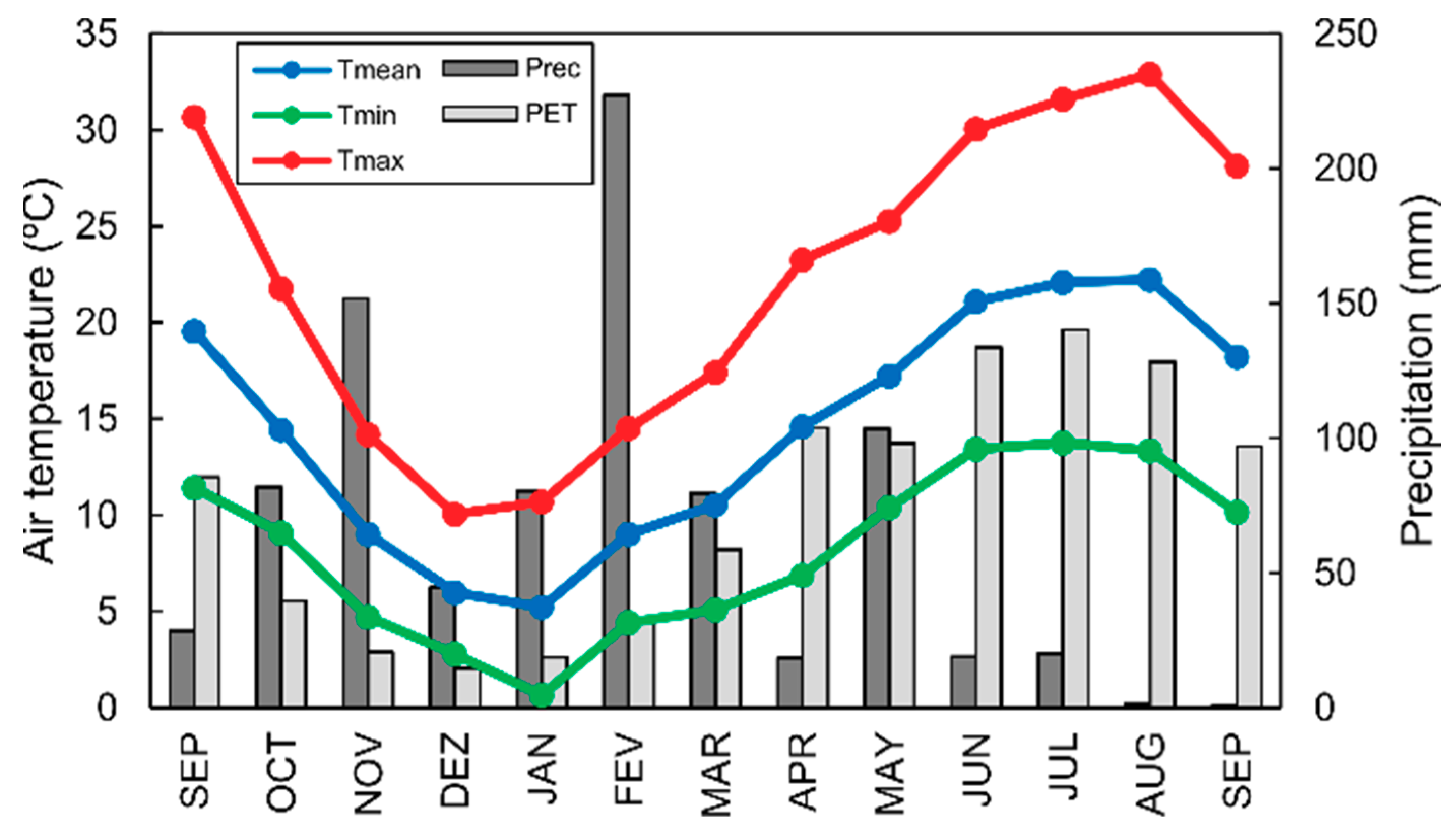
3.1. Study Area Characterization
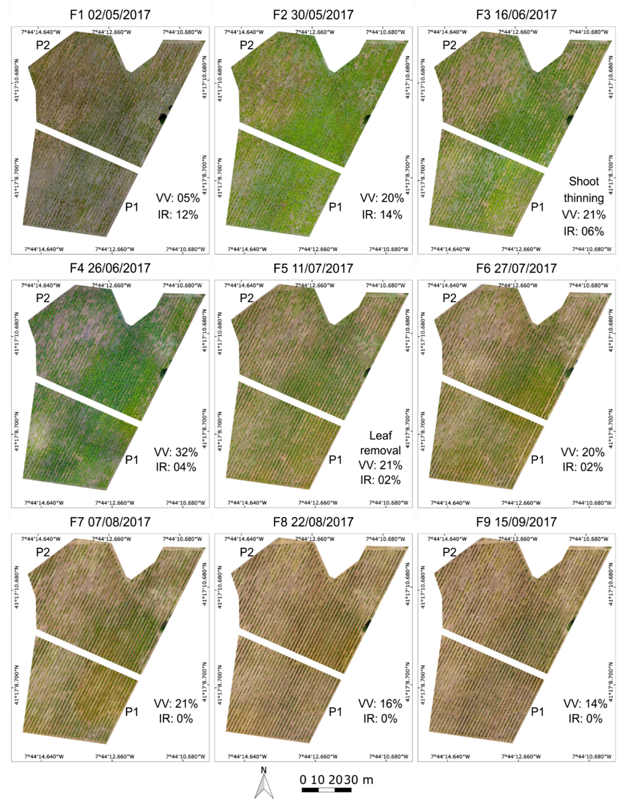
3.2. Vineyard Vegetation Change Monitoring
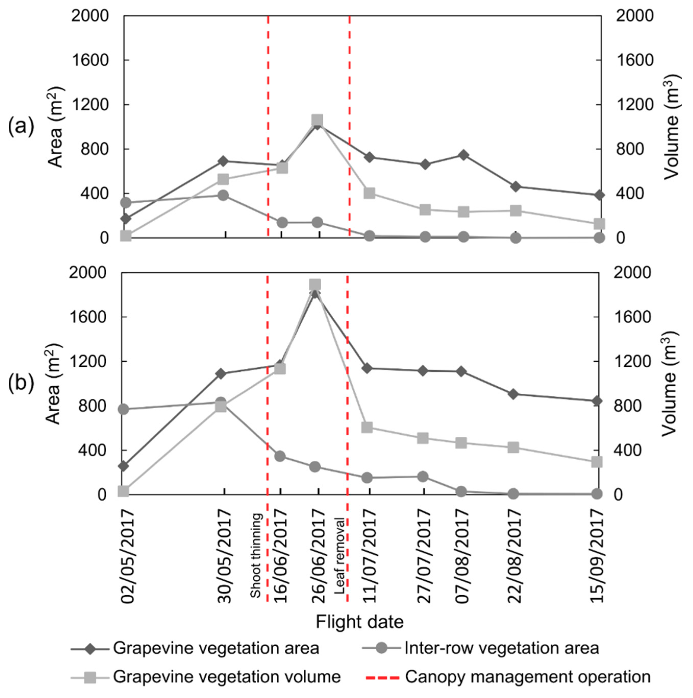
3.3. Multi-Temporal Analysis
3.4. Estimation of Vineyard Areas for Potential Canopy Management Operations
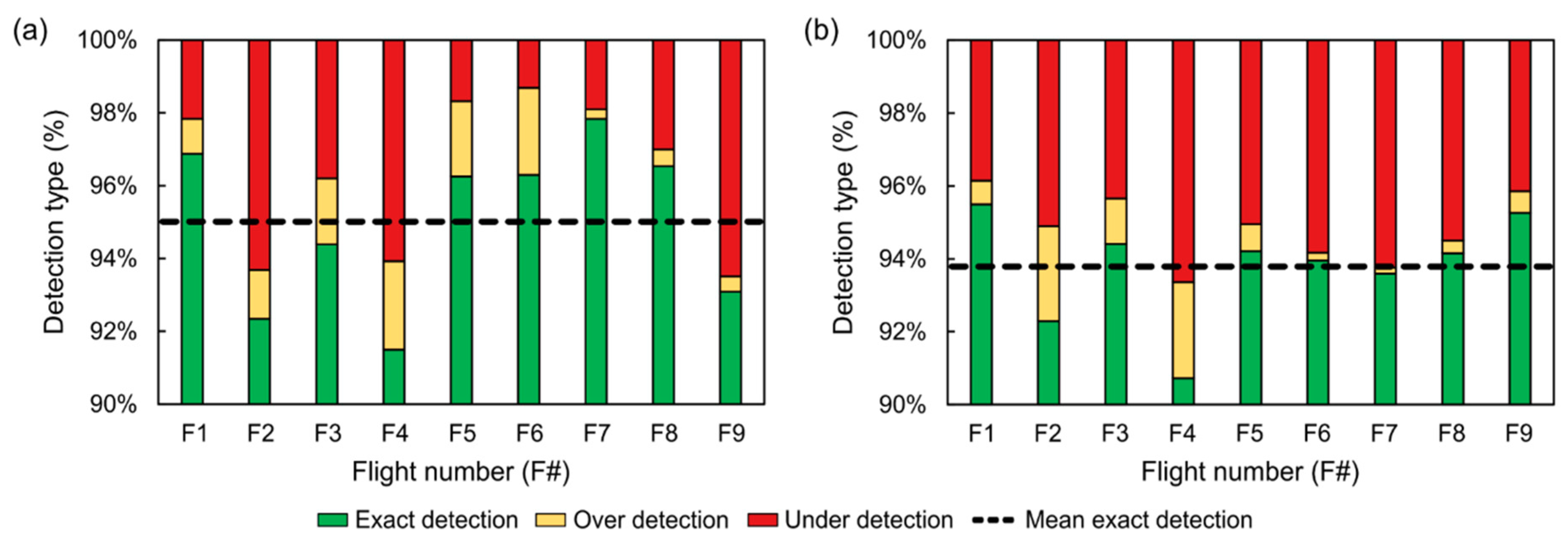
3.5. Accuracy Assessment
4. Discussion
4.1. Vegetation Evolution
4.2. Grapevine Row Height
4.3. Field Management Operations
5. Conclusions
Author Contributions
Funding
Acknowledgments
Conflicts of Interest
References
- Zarco-Tejada, P.J.; Hubbard, N.; Loudjani, P. Precision Agriculture: An Opportunity for EU Farmers—Potential Support with the CAP 2014–2020; Joint Research Centre (JRC) of the European Commission Monitoring Agriculture ResourceS (MARS): Brussels, Belgium, 2014. [Google Scholar]
- Ozdemir, G.; Sessiz, A.; Pekitkan, F.G. Precision viticulture tools to production of high quality grapes. Sci. Pap.-Ser. B-Hortic. 2017, 61, 209–218. [Google Scholar]
- Bramley, R.; Hamilton, R. Understanding variability in winegrape production systems. Aust. J. Grape Wine Res. 2004, 10, 32–45. [Google Scholar] [CrossRef]
- Bramley, R. Understanding variability in winegrape production systems 2. Within vineyard variation in quality over several vintages. Aust. J. Grape Wine Res. 2005, 11, 33–42. [Google Scholar] [CrossRef]
- Bramley, R.G.V. Progress in the development of precision viticulture—Variation in yield, quality and soil proporties in contrasting Australian vineyards. In Precision Tools for Improving Land Management; Fertilizer and Lime Research Centre: Palmerston North, New Zealand, 2001. [Google Scholar]
- Smart, R.E.; Dick, J.K.; Gravett, I.M.; Fisher, B.M. Canopy Management to Improve Grape Yield and Wine Quality—Principles and Practices. S. Afr. J. Enol. Viticult. 2017, 11, 3–17. [Google Scholar] [CrossRef]
- Vance, A.J.; Reeve, A.L.; Skinkis, P.A. The Role of Canopy Management in Vine Balance; Corvallis, or Extension Service, Oregon State University: Corvallis, OR, USA, 2013; p. 12. [Google Scholar]
- Bendig, J.; Bolten, A.; Bennertz, S.; Broscheit, J.; Eichfuss, S.; Bareth, G. Estimating Biomass of Barley Using Crop Surface Models (CSMs) Derived from UAV-Based RGB Imaging. Remote Sens. 2014, 6, 10395–10412. [Google Scholar] [CrossRef]
- CeSIA, A.D.G.; Corti, L.U.; Firenze, I. A simple model for simulation of growth and development in grapevine (Vitis vinifera L.). I. Model description. Vitis 1997, 36, 67–71. [Google Scholar]
- Duchêne, E.; Schneider, C. Grapevine and climatic changes: A glance at the situation in Alsace. Agron. Sustain. Dev. 2005, 25, 93–99. [Google Scholar] [CrossRef]
- Dobrowski, S.Z.; Ustin, S.L.; Wolpert, J.A. Remote estimation of vine canopy density in vertically shoot-positioned vineyards: Determining optimal vegetation indices. Aust. J. Grape Wine Res. 2008, 8, 117–125. [Google Scholar] [CrossRef]
- Yu, X.; Liang, X.; Hyyppä, J.; Kankare, V.; Vastaranta, M.; Holopainen, M. Stem biomass estimation based on stem reconstruction from terrestrial laser scanning point clouds. Remote Sens. Lett. 2013, 4, 344–353. [Google Scholar] [CrossRef]
- Kankare, V.; Holopainen, M.; Vastaranta, M.; Puttonen, E.; Yu, X.; Hyyppä, J.; Vaaja, M.; Hyyppä, H.; Alho, P. Individual tree biomass estimation using terrestrial laser scanning. ISPRS J. Photogramm. Remote Sens. 2013, 75, 64–75. [Google Scholar] [CrossRef]
- Matese, A.; Toscano, P.; Di Gennaro, S.F.; Genesio, L.; Vaccari, F.P.; Primicerio, J.; Belli, C.; Zaldei, A.; Bianconi, R.; Gioli, B. Intercomparison of UAV, Aircraft and Satellite Remote Sensing Platforms for Precision Viticulture. Remote Sens. 2015, 7, 2971–2990. [Google Scholar] [CrossRef]
- Pádua, L.; Vanko, J.; Hruška, J.; Adão, T.; Sousa, J.J.; Peres, E.; Morais, R. UAS, sensors, and data processing in agroforestry: A review towards practical applications. Int. J. Remote Sens. 2017, 38, 2349–2391. [Google Scholar] [CrossRef]
- Baofeng, S.; Jinru, X.; Chunyu, X.; Yulin, F.; Yuyang, S.; Fuentes, S. Digital surface model applied to unmanned aerial vehicle based photogrammetry to assess potential biotic or abiotic effects on grapevine canopies. Int. J. Agric. Biol. Eng. 2016, 9, 119. [Google Scholar]
- Baluja, J.; Diago, M.P.; Balda, P.; Zorer, R.; Meggio, F.; Morales, F.; Tardaguila, J. Assessment of vineyard water status variability by thermal and multispectral imagery using an unmanned aerial vehicle (UAV). Irrig. Sci. 2012, 30, 511–522. [Google Scholar] [CrossRef]
- Romero, M.; Luo, Y.; Su, B.; Fuentes, S. Vineyard water status estimation using multispectral imagery from an UAV platform and machine learning algorithms for irrigation scheduling management. Comput. Electron. Agric. 2018, 147, 109–117. [Google Scholar] [CrossRef]
- Santesteban, L.G.; Di Gennaro, S.F.; Herrero-Langreo, A.; Miranda, C.; Royo, J.B.; Matese, A. High-resolution UAV-based thermal imaging to estimate the instantaneous and seasonal variability of plant water status within a vineyard. Agric. Water Manag. 2017, 183, 49–59. [Google Scholar] [CrossRef]
- Kalisperakis, I.; Stentoumis, C.; Grammatikopoulos, L.; Karantzalos, K. Leaf area index estimation in vineyards from UAV hyperspectral data, 2D image mosaics and 3D canopy surface models. Int. Arch. Photogramm. Remote Sens. Spat. Inf. Sci. 2015, 40, 299. [Google Scholar] [CrossRef]
- Matese, A.; Di Gennaro, S.F.; Berton, A. Assessment of a canopy height model (CHM) in a vineyard using UAV-based multispectral imaging. Int. J. Remote Sens. 2016, 1–11. [Google Scholar] [CrossRef]
- Pölönen, I.; Saari, H.; Kaivosoja, J.; Honkavaara, E.; Pesonen, L. Hyperspectral Imaging Based Biomass and Nitrogen Content Estimations from Light-Weight UAV; SPIE: Bellingham, WA, USA, 2013; Volume 8887. [Google Scholar]
- Yue, J.; Yang, G.; Li, C.; Li, Z.; Wang, Y.; Feng, H.; Xu, B. Estimation of Winter Wheat Above-Ground Biomass Using Unmanned Aerial Vehicle-Based Snapshot Hyperspectral Sensor and Crop Height Improved Models. Remote Sens. 2017, 9, 708. [Google Scholar] [CrossRef]
- Capolupo, A.; Kooistra, L.; Berendonk, C.; Boccia, L.; Suomalainen, J. Estimating Plant Traits of Grasslands from UAV-Acquired Hyperspectral Images: A Comparison of Statistical Approaches. ISPRS Int. J. Geo-Inf. 2015, 4, 2792–2820. [Google Scholar] [CrossRef]
- Uto, K.; Seki, H.; Saito, G.; Kosugi, Y. Characterization of Rice Paddies by a UAV-Mounted Miniature Hyperspectral Sensor System. IEEE J. Sel. Top. Appl. Earth Obs. Remote Sens. 2013, 6, 851–860. [Google Scholar] [CrossRef]
- Näsi, R.; Honkavaara, E.; Lyytikäinen-Saarenmaa, P.; Blomqvist, M.; Litkey, P.; Hakala, T.; Viljanen, N.; Kantola, T.; Tanhuanpää, T.; Holopainen, M. Using UAV-Based Photogrammetry and Hyperspectral Imaging for Mapping Bark Beetle Damage at Tree-Level. Remote Sens. 2015, 7, 15467–15493. [Google Scholar] [CrossRef]
- Nevalainen, O.; Honkavaara, E.; Tuominen, S.; Viljanen, N.; Hakala, T.; Yu, X.; Hyyppä, J.; Saari, H.; Pölönen, I.; Imai, N.N.; et al. Individual Tree Detection and Classification with UAV-Based Photogrammetric Point Clouds and Hyperspectral Imaging. Remote Sens. 2017, 9, 185. [Google Scholar] [CrossRef]
- Adão, T.; Hruška, J.; Pádua, L.; Bessa, J.; Peres, E.; Morais, R.; Sousa, J.J. Hyperspectral Imaging: A Review on UAV-Based Sensors, Data Processing and Applications for Agriculture and Forestry. Remote Sens. 2017, 9, 1110. [Google Scholar] [CrossRef]
- Wallace, L.; Lucieer, A.; Watson, C.; Turner, D. Development of a UAV-LiDAR System with Application to Forest Inventory. Remote Sens. 2012, 4, 1519–1543. [Google Scholar] [CrossRef]
- Wallace, L.; Lucieer, A.; Watson, C.S. Evaluating Tree Detection and Segmentation Routines on Very High Resolution UAV LiDAR Data. IEEE Trans. Geosci. Remote Sens. 2014, 52, 7619–7628. [Google Scholar] [CrossRef]
- Chisholm, R.A.; Cui, J.; Lum, S.K.Y.; Chen, B.M. UAV LiDAR for below-canopy forest surveys. J. Unmanned Veh. Syst. 2013, 1, 61–68. [Google Scholar] [CrossRef]
- Zarco-Tejada, P.J.; Diaz-Varela, R.; Angileri, V.; Loudjani, P. Tree height quantification using very high resolution imagery acquired from an unmanned aerial vehicle (UAV) and automatic 3D photo-reconstruction methods. Eur. J. Agron. 2014, 55, 89–99. [Google Scholar] [CrossRef]
- Madec, S.; Baret, F.; de Solan, B.; Thomas, S.; Dutartre, D.; Jezequel, S.; Hemmerlé, M.; Colombeau, G.; Comar, A. High-Throughput Phenotyping of Plant Height: Comparing Unmanned Aerial Vehicles and Ground LiDAR Estimates. Front. Plant Sci. 2017, 8. [Google Scholar] [CrossRef] [PubMed]
- Sankey, T.; Donager, J.; McVay, J.; Sankey, J.B. UAV lidar and hyperspectral fusion for forest monitoring in the southwestern USA. Remote Sens. Environ. 2017, 195, 30–43. [Google Scholar] [CrossRef]
- Sankey, T.T.; McVay, J.; Swetnam, T.L.; McClaran, M.P.; Heilman, P.; Nichols, M. UAV hyperspectral and lidar data and their fusion for arid and semi-arid land vegetation monitoring. Remote Sens. Ecol. Conserv. 2018, 4, 20–33. [Google Scholar] [CrossRef]
- Von Bueren, S.; Yule, I. Multispectral aerial imaging of pasture quality and biomass using unmanned aerial vehicles (UAV). In Accurate and Efficient Use of Nutrients on Farms; Occasional Report; Fertilizer and Lime Research Centre, Massey University: Palmerston North, New Zealand, 2013; Volume 26. [Google Scholar]
- Vega, F.A.; Ramírez, F.C.; Saiz, M.P.; Rosúa, F.O. Multi-temporal imaging using an unmanned aerial vehicle for monitoring a sunflower crop. Biosyst. Eng. 2015, 132, 19–27. [Google Scholar] [CrossRef]
- Li, W.; Niu, Z.; Chen, H.; Li, D.; Wu, M.; Zhao, W. Remote estimation of canopy height and aboveground biomass of maize using high-resolution stereo images from a low-cost unmanned aerial vehicle system. Ecol. Indic. 2016, 67, 637–648. [Google Scholar] [CrossRef]
- Castaldi, F.; Pelosi, F.; Pascucci, S.; Casa, R. Assessing the potential of images from unmanned aerial vehicles (UAV) to support herbicide patch spraying in maize. Precis. Agric. 2017, 18, 76–94. [Google Scholar] [CrossRef]
- Schirrmann, M.; Giebel, A.; Gleiniger, F.; Pflanz, M.; Lentschke, J.; Dammer, K.-H. Monitoring Agronomic Parameters of Winter Wheat Crops with Low-Cost UAV Imagery. Remote Sens. 2016, 8, 706. [Google Scholar] [CrossRef]
- Bendig, J.; Yu, K.; Aasen, H.; Bolten, A.; Bennertz, S.; Broscheit, J.; Gnyp, M.L.; Bareth, G. Combining UAV-based plant height from crop surface models, visible, and near infrared vegetation indices for biomass monitoring in barley. Int. J. Appl. Earth Obs. Geoinf. 2015, 39, 79–87. [Google Scholar] [CrossRef]
- Moeckel, T.; Dayananda, S.; Nidamanuri, R.R.; Nautiyal, S.; Hanumaiah, N.; Buerkert, A.; Wachendorf, M. Estimation of Vegetable Crop Parameter by Multi-temporal UAV-Borne Images. Remote Sens. 2018, 10, 805. [Google Scholar] [CrossRef]
- Kim, D.-W.; Yun, H.S.; Jeong, S.-J.; Kwon, Y.-S.; Kim, S.-G.; Lee, W.S.; Kim, H.-J. Modeling and Testing of Growth Status for Chinese Cabbage and White Radish with UAV-Based RGB Imagery. Remote Sens. 2018, 10, 563. [Google Scholar] [CrossRef]
- Karpina, M.; Jarząbek-Rychard, M.; Tymków, P.; Borkowski, A. UAV-BASED AUTOMATIC TREE GROWTH MEASUREMENT FOR BIOMASS ESTIMATION. ISPRS Int. Arch. Photogramm. Remote Sens. Spat. Inf. Sci. 2016, XLI-B8, 685–688. [Google Scholar] [CrossRef]
- Carr, J.C.; Slyder, J.B. Individual tree segmentation from a leaf-off photogrammetric point cloud. Int. J. Remote Sens. 2018, 39, 5195–5210. [Google Scholar] [CrossRef]
- Mathews, A.J.; Jensen, J.L.R. Visualizing and Quantifying Vineyard Canopy LAI Using an Unmanned Aerial Vehicle (UAV) Collected High Density Structure from Motion Point Cloud. Remote Sens. 2013, 5, 2164–2183. [Google Scholar] [CrossRef]
- Mathews, A.J. Object-based spatiotemporal analysis of vine canopy vigor using an inexpensive unmanned aerial vehicle remote sensing system. J. Appl. Remote Sens. 2014, 8, 085199. [Google Scholar] [CrossRef]
- Weiss, M.; Baret, F. Using 3D Point Clouds Derived from UAV RGB Imagery to Describe Vineyard 3D Macro-Structure. Remote Sens. 2017, 9, 111. [Google Scholar] [CrossRef]
- Rouse, J.W., Jr.; Haas, R.H.; Schell, J.A.; Deering, D.W. Monitoring Vegetation Systems in the Great Plains with Erts. NASA Spec. Publ. 1974, 351, 309. [Google Scholar]
- Caruso, G.; Tozzini, L.; Rallo, G.; Primicerio, J.; Moriondo, M.; Palai, G.; Gucci, R. Estimating biophysical and geometrical parameters of grapevine canopies (‘Sangiovese’) by an unmanned aerial vehicle (UAV) and VIS-NIR cameras. VITIS J. Grapevine Res. 2017, 56. [Google Scholar] [CrossRef]
- De Castro, A.I.; Jiménez-Brenes, F.M.; Torres-Sánchez, J.; Peña, J.M.; Borra-Serrano, I.; López-Granados, F. 3-D Characterization of Vineyards Using a Novel UAV Imagery-Based OBIA Procedure for Precision Viticulture Applications. Remote Sens. 2018, 10, 584. [Google Scholar] [CrossRef]
- Pádua, L.; Adão, T.; Hruška, J.; Sousa, J.J.; Peres, E.; Morais, R.; Sousa, A. Very high resolution aerial data to support multi-temporal precision agriculture information management. Procedia Comput. Sci. 2017, 121, 407–414. [Google Scholar] [CrossRef]
- Magalhães, N. Tratado de Viticultura: A Videira, a Vinha eo Terroir; Chaves Ferreira: São Paulo, Brazil, 2008; ISBN 972-8987-15-3. [Google Scholar]
- Costa, R.; Fraga, H.; Malheiro, A.C.; Santos, J.A. Application of crop modelling to portuguese viticulture: Implementation and added-values for strategic planning. Ciência Téc. Vitiv. 2015, 30, 29–42. [Google Scholar] [CrossRef]
- Fraga, H.; Malheiro, A.C.; Moutinho-Pereira, J.; Cardoso, R.M.; Soares, P.M.M.; Cancela, J.J.; Pinto, J.G.; Santos, J.A. Integrated Analysis of Climate, Soil, Topography and Vegetative Growth in Iberian Viticultural Regions. PLoS ONE 2014, 9, e108078. [Google Scholar] [CrossRef] [PubMed]
- Johnson, L.F.; Roczen, D.E.; Youkhana, S.K.; Nemani, R.R.; Bosch, D.F. Mapping vineyard leaf area with multispectral satellite imagery. Comput. Electron. Agric. 2003, 38, 33–44. [Google Scholar] [CrossRef]
- Fraga, H.; Santos, J.A. Daily prediction of seasonal grapevine production in the Douro wine region based on favourable meteorological conditions. Aust. J. Grape Wine Res. 2017, 23, 296–304. [Google Scholar] [CrossRef]
- Burgos, S.; Mota, M.; Noll, D.; Cannelle, B. Use of very high-resolution airborne images to analyse 3D canopy architecture of a vineyard. Int. Arch. Photogramm. Remote Sens. Spat. Inf. Sci. 2015, 40, 399. [Google Scholar] [CrossRef]
- Comba, L.; Gay, P.; Primicerio, J.; Ricauda Aimonino, D. Vineyard detection from unmanned aerial systems images. Comput. Electron. Agric. 2015, 114, 78–87. [Google Scholar] [CrossRef]
- Nolan, A.; Park, S.; Fuentes, S.; Ryu, D.; Chung, H. Automated detection and segmentation of vine rows using high resolution UAS imagery in a commercial vineyard. In Proceedings of the 21st International Congress on Modelling and Simulation, Gold Coast, Australia, 29 November–4 December 2015; Volume 29, pp. 1406–1412. [Google Scholar]
- Poblete-Echeverría, C.; Olmedo, G.F.; Ingram, B.; Bardeen, M. Detection and Segmentation of Vine Canopy in Ultra-High Spatial Resolution RGB Imagery Obtained from Unmanned Aerial Vehicle (UAV): A Case Study in a Commercial Vineyard. Remote Sens. 2017, 9, 268. [Google Scholar] [CrossRef]
- Pádua, L.; Marques, P.; Hruška, J.; Adão, T.; Bessa, J.; Sousa, A.; Peres, E.; Morais, R.; Sousa, J.J. Vineyard properties extraction combining UAS-based RGB imagery with elevation data. Int. J. Remote Sens. 2018, 1–25. [Google Scholar] [CrossRef]
- Richardson, A.D.; Jenkins, J.P.; Braswell, B.H.; Hollinger, D.Y.; Ollinger, S.V.; Smith, M.-L. Use of digital webcam images to track spring green-up in a deciduous broadleaf forest. Oecologia 2007, 152, 323–334. [Google Scholar] [CrossRef] [PubMed]
- Otsu, N. A Threshold Selection Method from Gray-Level Histograms. IEEE Trans. Syst. Man Cybern. 1979, 9, 62–66. [Google Scholar] [CrossRef]


| Notation | Meaning |
|---|---|
| S | Binary image containing the central lines of the grapevine rows |
| Maximum height range used for crop surface model (CSM) thresholding | |
| Minimum height range used for CSM thresholding | |
| D | Binary image resultant from CSM and G% thresholding |
| F | Binary image resultant from the intersection of clusters of pixels in D with S |
| Set of all detected clusters in F | |
| Complement of F | |
| L | Binary image created from the intersection of with the thresholded G% binary image |
| A | Area of a given property to calculate (F or L), which is the sum of all pixel values (0 or 1) of a binary image with m n size, multiplied by the squared GSD value |
| Mean height of a given cluster , obtained from the CSM | |
| V | Grapevines’ vegetation volume, given by the area of clusters , multiplied by its mean height |
| k | Flight campaign number |
| X | Single-band image resultant from pixel-wise comparison of two consecutive flight campaigns (k and k + 1) |
| w | Maximum width that grapevines can assume |
| Flight Campaign (F#) | Mean Error (cm) | RMSE (cm) | ||||
|---|---|---|---|---|---|---|
| X | Y | Z | X | Y | Z | |
| F2 | 0.39 | 0.67 | −2.62 | 2.10 | 2.72 | 9.51 |
| F3 | −0.31 | −0.64 | 1.28 | 4.21 | 3.16 | 3.90 |
| F4 | −0.67 | 0.26 | −2.57 | 3.38 | 2.79 | 10.48 |
| F5 | 0.03 | 0.07 | −0.01 | 2.29 | 0.74 | 3.87 |
| F6 | −0.35 | −0.13 | −2.00 | 1.65 | 0.61 | 4.81 |
| F7 | −0.20 | −0.17 | −0.04 | 1.66 | 0.90 | 2.84 |
| F8 | −0.08 | −0.56 | −0.44 | 1.75 | 1.29 | 2.37 |
| F9 | −0.08 | −0.02 | −0.16 | 2.09 | 1.24 | 0.33 |
| Global | −0.16 | −0.06 | −0.82 | 2.54 | 1.93 | 5.78 |
| F#—Date (dd/mm/yyyy) | RMSE (m) | Overall | ||
|---|---|---|---|---|
| n = 50 | n = 37 | RMSE (m) | R2 | |
| F1—02/05/2017 | 0.20 | 0.19 | 0.13 | 0.78 |
| Shoot thinning F2—30/05/2017 | 0.15 | 0.14 | ||
| F3—16/06/2017 | 0.13 | 0.12 | ||
| Leaf removal F4—26/06/2017 | 0.14 | 0.13 | ||
| F5—11/07/2017 | 0.10 | 0.11 | ||
| F6—27/07/2017 | 0.10 | 0.10 | ||
| F7—07/08/2017 | 0.12 | 0.11 | ||
| F8—22/08/2017 | 0.12 | 0.12 | ||
| F9—15/09/2017 | 0.13 | 0.12 | ||
© 2018 by the authors. Licensee MDPI, Basel, Switzerland. This article is an open access article distributed under the terms and conditions of the Creative Commons Attribution (CC BY) license (http://creativecommons.org/licenses/by/4.0/).
Share and Cite
Pádua, L.; Marques, P.; Hruška, J.; Adão, T.; Peres, E.; Morais, R.; Sousa, J.J. Multi-Temporal Vineyard Monitoring through UAV-Based RGB Imagery. Remote Sens. 2018, 10, 1907. https://doi.org/10.3390/rs10121907
Pádua L, Marques P, Hruška J, Adão T, Peres E, Morais R, Sousa JJ. Multi-Temporal Vineyard Monitoring through UAV-Based RGB Imagery. Remote Sensing. 2018; 10(12):1907. https://doi.org/10.3390/rs10121907
Chicago/Turabian StylePádua, Luís, Pedro Marques, Jonáš Hruška, Telmo Adão, Emanuel Peres, Raul Morais, and Joaquim J. Sousa. 2018. "Multi-Temporal Vineyard Monitoring through UAV-Based RGB Imagery" Remote Sensing 10, no. 12: 1907. https://doi.org/10.3390/rs10121907
APA StylePádua, L., Marques, P., Hruška, J., Adão, T., Peres, E., Morais, R., & Sousa, J. J. (2018). Multi-Temporal Vineyard Monitoring through UAV-Based RGB Imagery. Remote Sensing, 10(12), 1907. https://doi.org/10.3390/rs10121907