Impacts of Climate Change and Intensive Lesser Snow Goose (Chen caerulescens caerulescens) Activity on Surface Water in High Arctic Pond Complexes


Abstract
1. Introduction
2. Materials and Methods
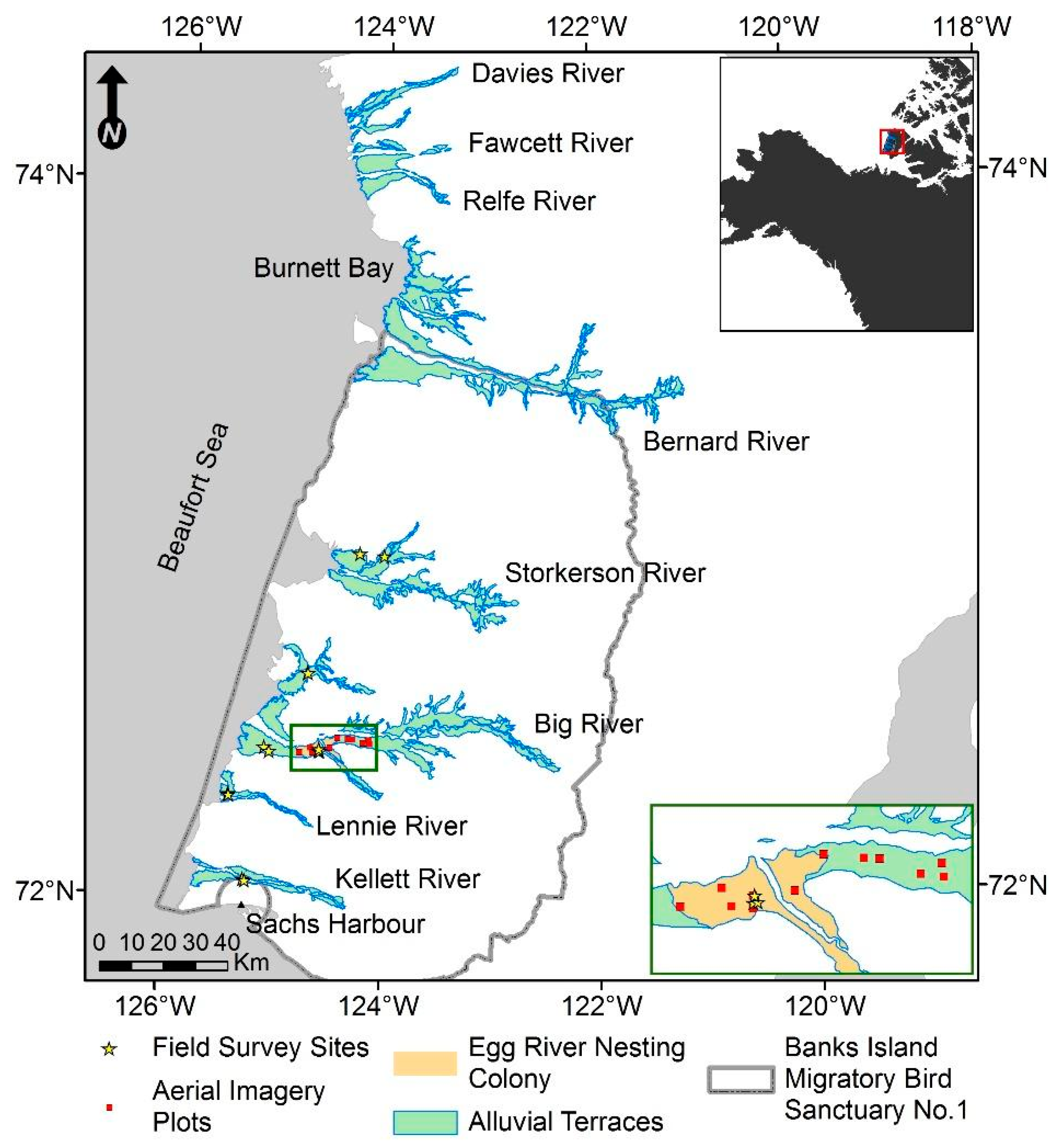
2.1. Study Area
2.2. Sub-Pixel Water Fraction
2.3. Fine-Scale Surface Water Change Detection
2.4. Field Surveys
3. Results
3.1. Sub-Pixel Water Fraction
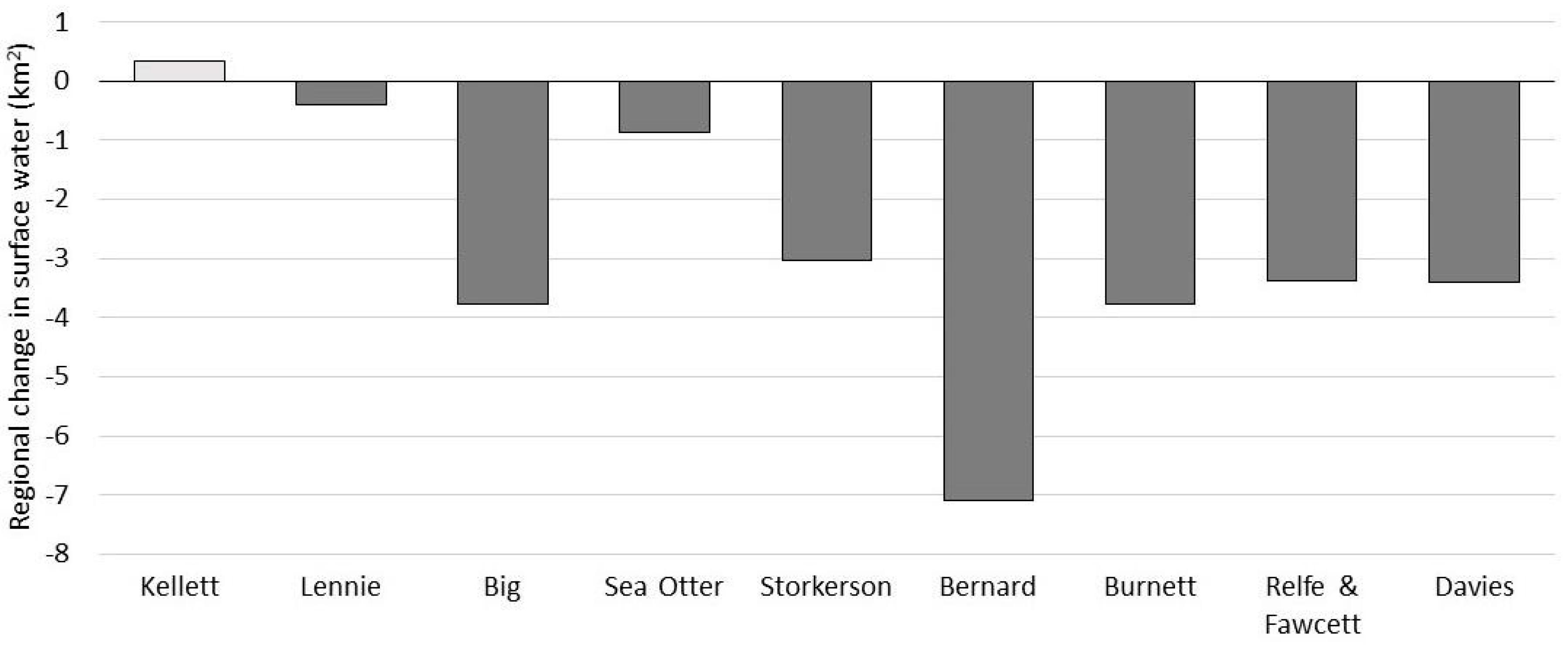
3.1.1. SWF Trends
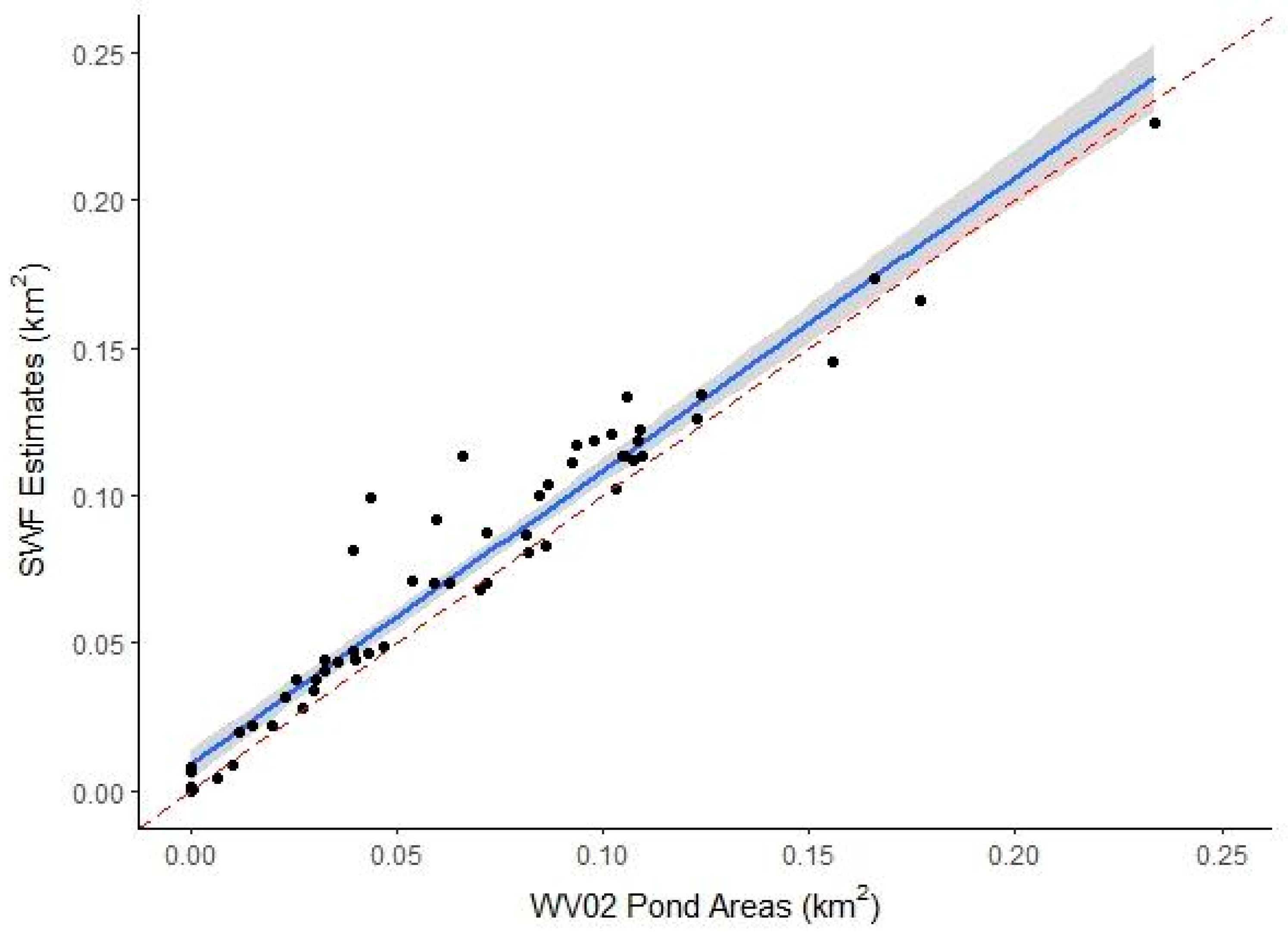
3.1.2. SWF Accuracy
3.2. Fine-Scale Surface Water Change Detection
3.2.1. Waterbody Size Distributions
3.2.2. Model Selection
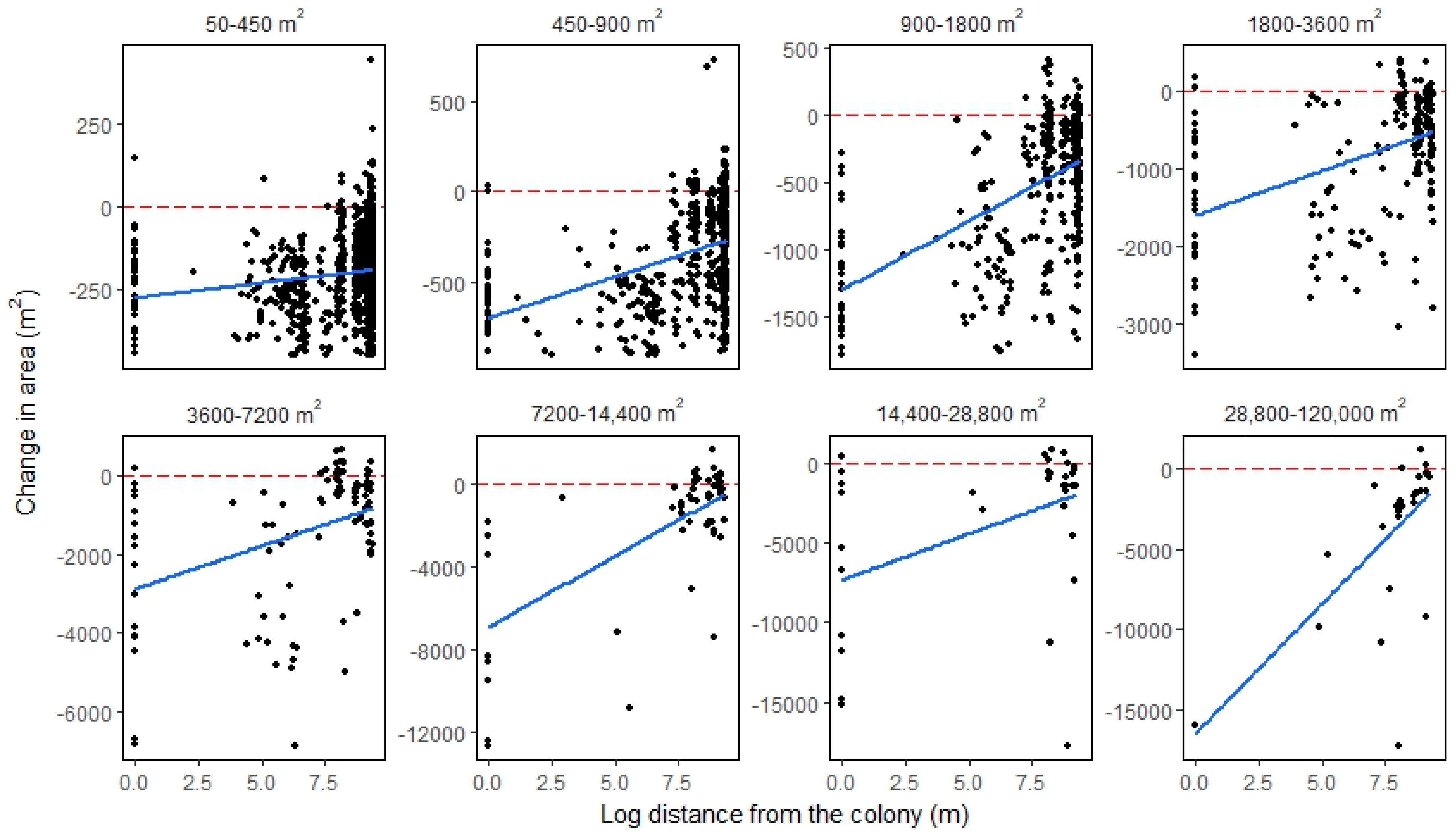
3.2.3. Categorical Proportional Area Loss
3.3. Field Surveys
3.3.1. Pond Basin Transect Intersections
3.3.2. Biotic and Abiotic Site Differences
4. Discussion
4.1. Smaller Waterbodies Are More Vulnerable
4.2. Intensified Drying in the Nesting Colony
4.3. Implications
5. Conclusions
- The pond complexes on western Banks Island are drying.
- Wetland drying is being caused by warming climate, but is exacerbated in areas with intensive snow goose habitat use.
- Future studies should explore the mechanisms causing pond desiccation, the impacts of snow geese on these processes, and the impacts of drying on vegetation and permafrost conditions.
- Remote sensing studies must use data and methods that consider the biophysical variation in the area of interest to adequately assess environmental changes.
Supplementary Materials
Author Contributions
Funding
Acknowledgments
Conflicts of Interest
Appendix A


References
- AMAP (Arctic Monitoring and Assessment Programme). Arctic Climate Issues 2011: Changes in Arctic Snow, WATER, ice and Permafrost; SWIPA 2011 Overview Report; AMAP: Oslo, Norway, 2012; p. 97. [Google Scholar]
- Pithan, F.; Mauritsen, T. Arctic amplification dominated by temperature feedbacks in contemporary climate models. Nat. Geosci. 2014, 7, 181–184. [Google Scholar] [CrossRef]
- Lantz, T.C.; Turner, K.W. Changes in lake area in response to thermokarst processes and climate in Old Crow Flats, Yukon. J. Geophys. Res. Biogeosci. 2015, 120, 513–524. [Google Scholar] [CrossRef]
- Kaplan, J.O.; New, M. Arctic climate change with a 2 °C global warming: Timing, climate patterns and vegetation change. Clim. Chang. 2006, 79, 213–241. [Google Scholar] [CrossRef]
- Bintanja, R.; Andry, O. Towards a rain-dominated Arctic. Nat. Clim. Chang. 2017, 7, 263–268. [Google Scholar] [CrossRef]
- Yoshikawa, K.; Hinzman, L.D. Shrinking thermokarst ponds and groundwater dynamics in discontinuous permafrost near Council Alaska. Permafr. Periglac. Process. 2003, 14, 151–160. [Google Scholar] [CrossRef]
- Nitze, I.; Grosse, G.; Jones, B.M.; Arp, C.D.; Ulrich, M.; Fedorov, A.; Veremeeva, A. Landsat-based trend analysis of lake dynamics across northern permafrost regions. Remote Sens. 2017, 9, 640. [Google Scholar] [CrossRef]
- Wolfe, B.B.; Light, E.M.; Macrae, M.L.; Hall, R.I.; Eichel, K.; Jasechko, S.; White, J.; Fishback, L.; Edwards, T.W.D. Divergent hydrological responses to 20th century climate change in shallow tundra ponds, western Hudson Bay Lowlands. Geophys. Res. Lett. 2011, 38, 1–6. [Google Scholar] [CrossRef]
- Negandhi, K.; Laurion, I.; Whiticar, M.J.; Galand, P.E.; Xu, X.; Lovejoy, C. Small thaw ponds: An unaccounted source of methane in the Canadian high Arctic. PLoS ONE 2013, 8, e78204. [Google Scholar] [CrossRef] [PubMed]
- Becker, M.S.; Davies, T.J.; Pollard, W.H. Ground ice melt in the high Arctic leads to greater ecological heterogeneity. J. Ecol. 2016, 104, 114–124. [Google Scholar] [CrossRef]
- Slattery, S.M.; Alisauskas, R.T. Distribution and habitat use of Ross’ and lesser snow geese during late brood rearing. J. Wildl. Manag. 2007, 71, 2230–2237. [Google Scholar] [CrossRef]
- Anthony, K.W.; Daanen, R.; Anthony, P.; Schneider von Deimling, T.; Ping, C.-L.; Chanton, J.P.; Grosse, G. Methane emissions proportional to permafrost carbon thawed in Arctic lakes since the 1950s. Nat. Geosci. 2016, 9, 679–685. [Google Scholar] [CrossRef]
- White, D.; Hinzman, L.; Alessa, L.; Cassano, J.; Chambers, M.; Falkner, K.; Francis, J.; Gutowski, W.J., Jr.; Holland, M.; Holmes, R.M.; et al. The arctic freshwater system: Changes and impacts. J. Geophys. Res. 2007, 112, G04S54. [Google Scholar] [CrossRef]
- Raymond, P.A.; Hartmann, J.; Lauerwald, R.; Sobek, S.; McDonald, C.; Hoover, M.; Butman, D.; Striegl, R.; Mayorga, E.; Humborg, C.; et al. Global carbon dioxide emissions from inland waters. Nature 2013, 503, 355–387. [Google Scholar] [CrossRef] [PubMed]
- Smol, J.P.; Douglas, S.V. Crossing the final ecological threshold in high Arctic ponds. PNAS 2007, 104, 12395–12397. [Google Scholar] [CrossRef] [PubMed]
- Plug, L.J.; Walls, C.; Scott, B.M. Tundra lake changes from 1978 to 2001 on the Tuktoyaktuk Peninsula, western Canadian Arctic. Geophys. Res. Lett. 2008, 35, L03502. [Google Scholar] [CrossRef]
- Smith, L.C.; Sheng, Y.; MacDonald, G.M.; Hinzman, L.D. Disappearing Arctic lakes. Science 2005, 308, 1429. [Google Scholar] [CrossRef] [PubMed]
- Jones, B.M.; Grosse, G.; Arp, C.D.; Jones, M.C.; Anthony, K.M.W.; Romanovsky, V.E. Modern thermokarst lake dynamics in the continuous permafrost zone, northern Seward Peninsula, Alaska. J. Geophys. Res. 2011, 116, G00M03. [Google Scholar] [CrossRef]
- Olthof, I.; Fraser, R.H.; Schmitt, C. Landsat-based mapping of thermokarst lake dynamics on the Tuktoyaktuk coastal plain: Northwest Territories, Canada since 1985. Remote Sens. Environ. 2015, 168, 194–204. [Google Scholar] [CrossRef]
- Arp, C.D.; Jones, B.M.; Urban, F.E.; Grosse, G. Hydrogeomorphic processes of thermokarst lakes with grounded-ice and floating-ice regimes on the Arctic coastal plain, Alaska. Hydrol. Process. 2011, 25, 2422–2438. [Google Scholar] [CrossRef]
- Marsh, P.; Bigras, S.C. Evaporation from Mackenzie Delta lakes, N.W.T., Canada. Arct. Alp. Res. 1988, 20, 220–229. [Google Scholar] [CrossRef]
- Turner, K.W.; Wolfe, B.B.; Edwards, T.E.; Lantz, T.C.; Hall, R.I.; La Rocque, G. Controls on water balance of shallow thermokarst lakes and their relations with catchment characteristics: A multi-year, landscape-scale assessment based on water isotope tracers and remote sensing in Old Crow Flats, Yukon (Canada). Glob. Chang. Boil. 2014, 20, 1585–1603. [Google Scholar] [CrossRef]
- Roach, J.K.; Griffith, B.; Verbyla, D. Landscape influences on climate-related lake shrinkage at high latitudes. Glob. Chang. Boil. 2013, 19, 2276–2284. [Google Scholar] [CrossRef] [PubMed]
- Carroll, M.L.; Townshend, J.R.G.; DiMiceli, C.M.; Loboda, T.; Sohlberg, R.A. Shrinking lakes of the Arctic: Spatial relationships and trajectory of change. Geophys. Res. Lett. 2011, 38, 1–5. [Google Scholar] [CrossRef]
- Riordan, B.; Verbyla, D.; McGuire, A.D. Shrinking ponds in subarctic Alaska based on 1950–2002 remotely sensed images. J. Geophys. Res. 2006, 111, G04002. [Google Scholar] [CrossRef]
- Woo, M.-K.; Young, K.L. High Arctic wetlands: Their occurrence, hydrological characteristics and sustainability. J. Hydrol. 2006, 320, 432–450. [Google Scholar] [CrossRef]
- Abnizova, A.; Young, K.L. Sustainability of high Arctic ponds in a polar desert environment. Arctic 2010, 63, 67–84. [Google Scholar] [CrossRef]
- Woo, M.-K.; Young, K.L.; Brown, L. High Arctic patchy wetlands: Hydrological variability and their sustainability. Phys. Geogr. 2006, 27, 297–307. [Google Scholar] [CrossRef]
- Steedman, A.E.; Lantz, T.C.; Kokelj, S.V. Spatio-temporal variation in high-centre polygons and ice-wedge melt ponds, Tuktoyaktuk Coastlands, Northwest Territories. Permafr. Periglac. Process. 2017, 28, 66–78. [Google Scholar] [CrossRef]
- Fraser, R.H.; Kokelj, S.V.; Lantz, T.C.; McFarlane-Winchester, M.; Olthof, I.; Lacelle, D. Climate sensitivity of high Arctic permafrost terrain demonstrated by widespread ice-wedge thermokarst on Banks Island. Remote Sens. 2018, 10, 954. [Google Scholar] [CrossRef]
- Hines, J.E.; Latour, P.B.; Squires-Taylor, C.; Moore, S. The Effects on Lowland Habitat in the Banks Island Bird Sanctuary Number 1, Northwest Territories, by the Growing Colony of Lesser Snow Geese (Chen caerulescens caerulescens); Environment Canada Occasional Paper 118; Environment Canada, Canadian Wildlife Service: Edmonton, AB, Canada, 2010; pp. 8–26.
- Batt, B.D.J. Arctic Ecosystems in Peril: Report of the Arctic Goose Habitat Working Group; Arctic Goose Joint Venture Special Publication; U.S. Fish and Wildlife Service: Washington, DC, USA; Canadian Wildlife Service: Ottawa, ON, Canada, 1997; pp. 1–12. ISBN 0961727934.
- Kotanen, P.M.; Jefferies, R.L. Long-term destruction of sub-arctic wetland vegetation by lesser snow geese. Ecoscience 1997, 4, 179–182. [Google Scholar] [CrossRef]
- Srivastava, D.S.; Jefferies, R.L. A positive feedback: Herbivory, plant growth, salinity, and the desertification of an Arctic salt-marsh. J. Ecol. 1996, 84, 31–42. [Google Scholar] [CrossRef]
- Calvert, A.M. Interactions between Light Geese and Northern Flora and Fauna: Synthesis and Assessment of Potential Impacts; Unpublished Report; Environment Canada: Ottawa, ON, Canada, 2015; pp. 1–37.
- Jefferies, R.L.; Jensen, A.; Abraham, K.F. Vegetational development and the effect of geese on vegetation at La Perouse Bay, Manitoba. Can. J. B 1979, 57, 1439–1450. [Google Scholar] [CrossRef]
- Iacobelli, A.; Jefferies, R.L. Inverse salinity gradients in coastal marshes and the death of stands of Salix: The effects of grubbing by geese. J. Ecol. 1991, 79, 61–73. [Google Scholar] [CrossRef]
- Park, J.S. A race against time: Habitat alteration by snow geese prunes the seasonal sequence of mosquito emergence in a subarctic brackish landscape. Polar Biol. 2017, 40, 553–561. [Google Scholar] [CrossRef]
- Mudryk, L.R.; Derksen, C.; Howell, S.; Laliberte, F.; Thackeray, C.; Sospedra-Alfonso, R.; Vionnet, V.; Kushner, P.J.; Brown, R. Canadian snow and sea ice: Historical trends and projections. Cryosphere 2018, 12, 1157–1176. [Google Scholar] [CrossRef]
- Lakeman, T.R.; England, J.H. Late Wisconsinan glaciation and postglacial relative sea-level change on western Banks Island, Canadian Arctic Archipelago. Quat. Res. 2013, 80, 99–112. [Google Scholar] [CrossRef]
- Ecosystem Classification Group. Ecological Regions of the Northwest Territories—Northern Arctic; Department of Environment and Natural Resources, Government of the Northwest Territories: Yellowknife, NT, Canada, 2013; pp. 1–157. ISBN 978–0-7708-0205-9.
- Chander, G.; Markham, B.L.; Helder, D.L. Summary of current radiometric calibration coefficients for Landsat MSS, TM, ETM+, and EO-1 ALI sensors. Remote Sens. Environ. 2009, 113, 893–903. [Google Scholar] [CrossRef]
- Crist, E.P.; Cicone, R.C. A physically-based transformation of thematic mapper data—The TM tasseled cap. IEEE Trans. Geosci. Remote Sens. 1984, GE-22, 256–263. [Google Scholar] [CrossRef]
- Huang, C.; Wylie, B.; Yang, L.; Homer, C.; Zylstra, G. Derivation of a tasseled cap transformation based on Landsat 7 at-satellite reflectance. Int. J. Remote Sens. 2002, 23, 1741–1748. [Google Scholar] [CrossRef]
- Kauth, R.J.; Thomas, G.S. The tasseled cap—A graphic description of the spectral-temporal development of agricultural crops as seen by Landsat. LARS Symp. 1976, 159, 41–51. [Google Scholar]
- Zeileis, A.; Leisch, F.; Hornik, K.; Kleiber, C. Strucchange: An R package for testing for structural change in linear regression models. J. Stat. Softw. 2002, 7, 1–38. [Google Scholar] [CrossRef]
- R Core Team. R: A Language and Environment for Statistical Computing. R Foundation for Statistical Computing, Vienna, Austria, 2016. Available online: https://www.R-project.org/ (accessed on 18 March 2018).
- Bai, J.; Perron, P. Computation and analysis of multiple structural change models. J. Appl. Econ. 2003, 18, 1–22. [Google Scholar] [CrossRef]
- Fraser, R.H.; Olthof, I.; Kokelj, S.V.; Lantz, T.C.; Lacelle, D.; Brooker, A.; Wolfe, S.; Schwarz, S. Detecting landscape changes in high latitude environments using Landsat trend analysis: 1. Visualization. Remote Sens. 2014, 6, 11533–11557. [Google Scholar] [CrossRef]
- Kendall, M.G.; Stuart, A.S. Advanced Theory of Statistics; Charles Griffin and Company: London, UK, 1967; Volume 2. [Google Scholar]
- Noh, M.-J.; Howat, I.M. Automated stereo-photogrammetric DEM generation at high latitudes: Surface extraction with TIN-based search-space minimization (SETSM) validation and demonstration over glaciated regions. GISci. Remote Sens. 2015, 52, 198–217. [Google Scholar] [CrossRef]
- Anselin, L. Local indicators of spatial association—LISA. Geogr. Anal. 1995, 27, 93–115. [Google Scholar] [CrossRef]
- Anselin, L. GeoDa: An introduction to spatial data analysis. Geogr. Anal. 2005, 38, 5–22. [Google Scholar] [CrossRef]
- Burnham, K.P.; Anderson, D.R. Model Selection and Multimodel Inference: A Practical Information-Theoretic Approach, 2nd ed.; Springer: New York, NY, USA, 2002; ISBN 0-387-95364-7. [Google Scholar]
- Zuur, A.F.; Ieno, E.N.; Elphick, C.S. A protocol for data exploration to avoid common statistical problems. Methods Ecol. Evol. 2010, 1, 3–14. [Google Scholar] [CrossRef]
- Graham, M.H. Confronting multicollinearity in ecological multiple regression. Ecology 2003, 84, 2809–2815. [Google Scholar] [CrossRef]
- Littell, R.C.; Milliken, G.A.; Stroup, W.W.; Wolfinger, R.D.; Schabenberger, O. SAS for Mixed Models, 2nd ed.; SAS Institute Inc.: Carry, NC, USA, 2006; ISBN 978-1-59047-500-3. [Google Scholar]
- Samelius, G.; Alisauskas, R.T.; Hines, J.E. Productivity of Lesser Snow Geese on Banks Island, Northwest Territories, Canada, in 1995–1998; Environment Canada Occasional Paper 115; Environment Canada, Canadian Wildlife Service: Edmonton, AB, Canada, 2008; pp. 3–33.
- Price, L.W. Vegetation, microtopography, and depth of active layer on different exposures in subarctic alpine tundra. Ecology 1971, 52, 638–647. [Google Scholar] [CrossRef] [PubMed]
- Fisher, J.P.; Estop-Aragones, C.; Thierry, A.; Charman, D.J.; Wolfe, S.A.; Hartley, I.P.; Murton, J.B.; Williams, M.; Phoenix, G.K. The influence of vegetation and soil characteristics on active-layer thickness of permafrost soils in boreal forest. Glob. Chang. Boil. 2016, 22, 3127–3140. [Google Scholar] [CrossRef] [PubMed]
- Gornall, J.L.; Jonsdottir, I.S.; Woodin, S.J.; Van der Wal, R. Arctic mosses govern below-ground environment and ecosystem processes. Oecologia 2007, 153, 931–941. [Google Scholar] [CrossRef] [PubMed]
- Woo, M.-K.; Guan, X.J. Hydrological connectivity and seasonal storage change of tundra ponds in a polar oasis environment, Canadian high Arctic. Permafr. Periglac. Process. 2006, 17, 309–323. [Google Scholar] [CrossRef]
- Kokelj, S.V.; Jorgenson, M.T. Advances in thermokarst research. Permafr. Periglac. Process. 2013, 24, 108–119. [Google Scholar] [CrossRef]
- Suzuki, K.; Matsuo, K.; Yamakazi, D.; Ichii, K.; Iijima, Y.; Papa, F.; Yanagi, Y.; Hiyama, T. Hydrological variability and changes in the Arctic circumpolar tundra and the three largest pan-Arctic river basins from 2002 to 2016. Remote Sens. 2018, 10, 402. [Google Scholar] [CrossRef]
- Brown, L.; Young, K.L. Assessment of three mapping techniques to delineate lakes and ponds in a Canadian high Arctic wetland complex. Arctic 2006, 59, 283–293. [Google Scholar] [CrossRef]
- Liljedahl, A.K.; Boike, J.; Daanen, R.P.; Fedorov, A.N.; Frost, G.V.; Grosse, G.; Hinzman, L.D.; Iijma, Y.; Jorgenson, J.C.; Matveyeva, N.; et al. Pan-Arctic ice-wedge degradation in warming permafrost and its influence on tundra hydrology. Nat. Geosci. 2016, 9, 312–319. [Google Scholar] [CrossRef]
- Riedlinger, D.; Berkes, F. Contributions of traditional knowledge to understanding climate change in the Canadian Arctic. Polar Rec. 2001, 37, 315–328. [Google Scholar] [CrossRef]
- Ashford, G.; Catleden, J. Inuit Observations on Climate Change: Final Report; International Institute for Sustainable Development: Winnipeg, MB, Canada, 2001; pp. 1–31. [Google Scholar]
- Ferguson, M.A.D.; Messier, F. Collection and analysis of traditional ecological knowledge about a population of Arctic tundra caribou. Arctic 1997, 50, 17–28. [Google Scholar] [CrossRef]
- Pekel, J.-F.; Cottam, A.; Gorelick, N.; Belward, A.S. High-resolution mapping of global surface water and its long-term changes. Nature 2016, 540, 418–422. [Google Scholar] [CrossRef] [PubMed]
- French, H.M. The Periglacial Environment, 3rd ed.; John Wiley & Sons: Chichester, UK, 2007; ISBN 978-0-47086-588-0. [Google Scholar]
- Lachenbruch, A.H. Mechanics of Thermal Contraction Cracks and Ice-Wedge Polygons in Permafrost; Geological Society of America Special Papers; Geological Society of America: Boulder, CO, USA, 1962; Volume 70, pp. 1–66. [Google Scholar] [CrossRef]
- Martin, A.F.; Lantz, T.C.; Humphreys, E.R. Ice wedge degradation and CO2 and CH4 emissions in the Tuktoyaktuk coastlands, Northwest Territories. Arct. Sci. 2018, 4, 130–145. [Google Scholar] [CrossRef]


| Hypothesis | Parameter | Description | Impact (+/-) | Model Number and Statement | Citation |
|---|---|---|---|---|---|
| Size: Smaller ponds are more vulnerable to change and climatic variability, compared to larger ponds. | Pond size | Waterbody extent from the 1958 aerial photographs. | + | (1) Area change ~ Pond size | [15,20,21] |
| Vegetation: Vegetation cover insulates near-surface ground temperatures and increases soil water retention, sustaining subsurface hydrological connectivity and reducing system water loss through evaporation. | 2015 TCG | Average TCG value within 0–25 m of the waterbody, taken from a 18 July 2015 Landsat scene. | + | (2) Area change ~ 2015 TCG | [28,59,60,61,62] |
| (3) Area change ~ 2015 TCG + Pond size | |||||
| (4) Area change ~ 2015 TCG + Pond size + 2015 TCG × Pond size | |||||
| Herbivore intensity: Intensive and recurring goose foraging can alter microtopography, and increase soil temperature and evaporation levels, which may reduce hydroperiod in nearby waterbodies or increase risk of drainage. | Colony distance | Distance from the nesting colony, which was delineated as areas of high snow goose density, using data from Samelius et al. [58]. | + | (5) Area change ~ log(Colony distance) | [34,36,37,38] |
| (6) Area change ~ log(Colony distance) + Pond size | |||||
| (7) Area change ~ log(Colony distance) + Pond size + log(Colony distance) × Pond size | |||||
| Surface water connectivity: Drainage areas will have higher levels of thermal erosion gullying and are more likely to experience lateral drainage. | Flow accumulation | Maximum flow level within 25 m of the waterbody, based on the number of upslope pixels. | - | (8) Area change ~ Flow accumulation | [63] |
| (9) Area change ~ Flow accumulation + Pond size | |||||
| (10) Area change ~ Flow accumulation + Pond size + Flow accumulation × Pond size |
| Severe Drying | Stable | |||
|---|---|---|---|---|
| Observed | Expected | Observed | Expected | |
| 50–450 m2 | 625 | 597 | 324 | 352 |
| 450–900 m2 | 455 * | 402 | 184 * | 237 |
| 900–1800 m2 | 249 | 255 | 156 | 150 |
| 1800–3600 m2 | 100 * | 121 | 93 * | 72 |
| 3600–7200 m2 | 53 | 64 | 49 | 38 |
| 7200–14,400 m2 | 15 * | 35 | 41 * | 21 |
| 14,400–28,800 m2 | 14 * | 23 | 22 * | 13 |
| 28,800–120,000 m2 | 4 * | 18 | 25 * | 11 |
| Column totals | 1515 | 1515 | 894 | 894 |
| Waterbody Size in 1958 (m2) | 50–450 | 450–900 | 900–1800 | 1800–3600 | 3600–7200 | 7200–14,400 | 14,400–28,800 | 28,800–120,000 |
|---|---|---|---|---|---|---|---|---|
| Count | 949 | 639 | 405 | 193 | 102 | 56 | 36 | 29 |
| Total area (m2) | 213,525 | 431,325 | 546,750 | 521,100 | 550,800 | 604,800 | 777,600 | 2,157,600 |
| Change in total area (m2) | −193,437 | −212,536 | −204,329 | −153,752 | −151,374 | −119,682 | −142,308 | −107,254 |
| Proportion of total area lost | 90.59% | 49.28% | 37.37% | 29.51% | 27.48% | 19.79% | 18.30% | 4.97% |
| Model Number | Explanatory Variables | R2 | AICc | ΔAICc | AICc Weight | Rank |
|---|---|---|---|---|---|---|
| 7 | log(Colony Distance) + Pond Size + log(Colony Distance) × Pond Size | 0.429 | 39960.4 | 0 | 1.0 | 1 |
| 6 | log(Colony Distance) + Pond Size | 0.291 | 40482.6 | 522.2 | 4.0 × 10−114 | 2 |
| 4 | 2015 TCG + Pond Size + 2015 TCG × Pond Size | 0.276 | 40532.4 | 572.0 | 6.2 × 10−125 | 3 |
| 3 | 2015 TCG + Pond Size | 0.220 | 40710.3 | 749.9 | 1.4 × 10−163 | 4 |
| 1 | Pond Size | 0.211 | 40739.5 | 779.1 | 6.5 × 10−170 | 5 |
| 9 | Flow Accumulation + Pond Size | 0.210 | 40741.0 | 780.6 | 3.1 × 10−170 | 6 |
| 10 | Flow Accumulation + Pond Size + Flow Accumulation × Pond Size | 0.210 | 40742.5 | 782.1 | 1.4 × 10−170 | 7 |
| 5 | log(Colony Distance) | 0.0995 | 41056.4 | 1096.0 | 9.8 × 10−239 | 8 |
| 2 | 2015 TCG | 0.00926 | 41286.4 | 1326.0 | 1.1 × 10−288 | 9 |
| 8 | Flow Accumulation | 0.00264 | 41302.5 | 1342.1 | 3.6 × 10−292 | 10 |
© 2018 by the authors. Licensee MDPI, Basel, Switzerland. This article is an open access article distributed under the terms and conditions of the Creative Commons Attribution (CC BY) license (http://creativecommons.org/licenses/by/4.0/).
Share and Cite
Campbell, T.K.F.; Lantz, T.C.; Fraser, R.H. Impacts of Climate Change and Intensive Lesser Snow Goose (Chen caerulescens caerulescens) Activity on Surface Water in High Arctic Pond Complexes. Remote Sens. 2018, 10, 1892. https://doi.org/10.3390/rs10121892
Campbell TKF, Lantz TC, Fraser RH. Impacts of Climate Change and Intensive Lesser Snow Goose (Chen caerulescens caerulescens) Activity on Surface Water in High Arctic Pond Complexes. Remote Sensing. 2018; 10(12):1892. https://doi.org/10.3390/rs10121892
Chicago/Turabian StyleCampbell, T. Kiyo F., Trevor C. Lantz, and Robert H. Fraser. 2018. "Impacts of Climate Change and Intensive Lesser Snow Goose (Chen caerulescens caerulescens) Activity on Surface Water in High Arctic Pond Complexes" Remote Sensing 10, no. 12: 1892. https://doi.org/10.3390/rs10121892
APA StyleCampbell, T. K. F., Lantz, T. C., & Fraser, R. H. (2018). Impacts of Climate Change and Intensive Lesser Snow Goose (Chen caerulescens caerulescens) Activity on Surface Water in High Arctic Pond Complexes. Remote Sensing, 10(12), 1892. https://doi.org/10.3390/rs10121892