An Improved Boosting Learning Saliency Method for Built-Up Areas Extraction in Sentinel-2 Images


Abstract
:1. Introduction
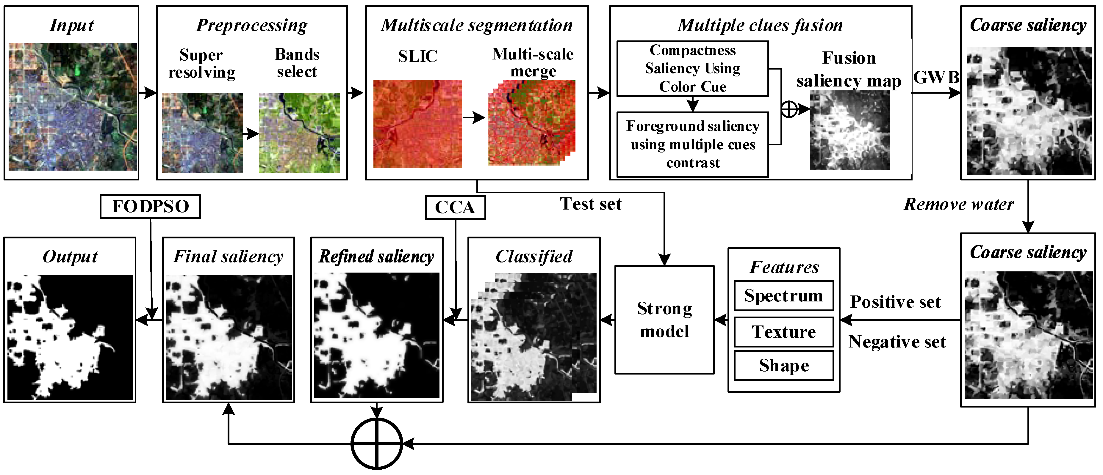
2. Proposed Method
2.1. Image Preprocessing
2.1.1. Sentinel-2 Constellation
2.1.2. Atmospheric Correction and Image Sharpening
2.1.3. Optimal Band Selection
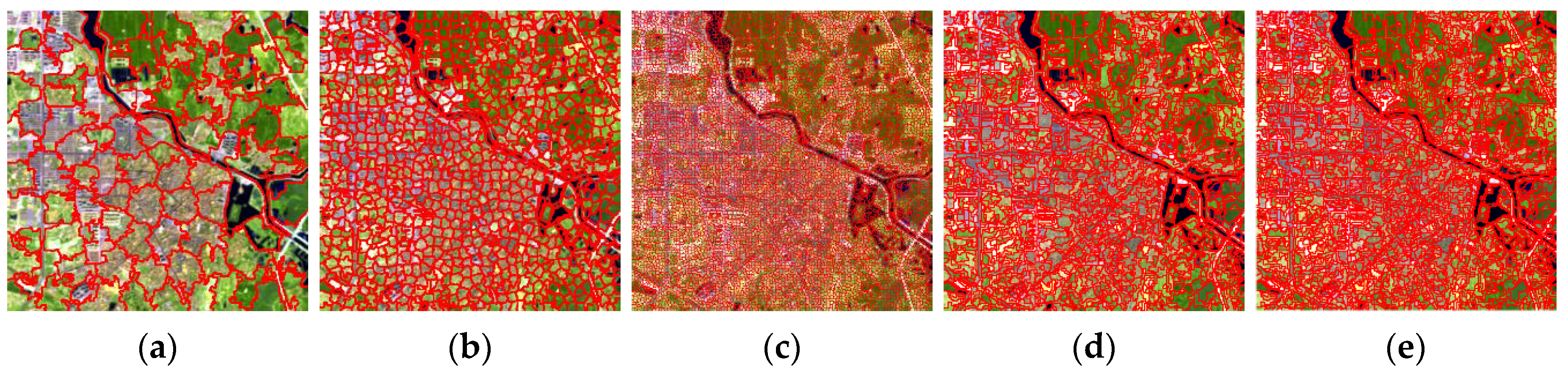
2.2. Multiscale Segmentation
2.3. Feature Selection
2.4. Coarse Saliency Map
2.4.1. Multiple Cues Fusion
Compactness Saliency Using Color Cues
Foreground Saliency Using Multiple Cues Contrast
2.4.2. Geodesic Weighted Bayesian
2.4.3. Removing the Water Bodies
2.4.4. Training Sample Selection
2.5. Refined Saliency Map
2.6. Multiscale Saliency
2.7. Integration
2.8. Bulit-Up Area Extraction
3. Experimental Results
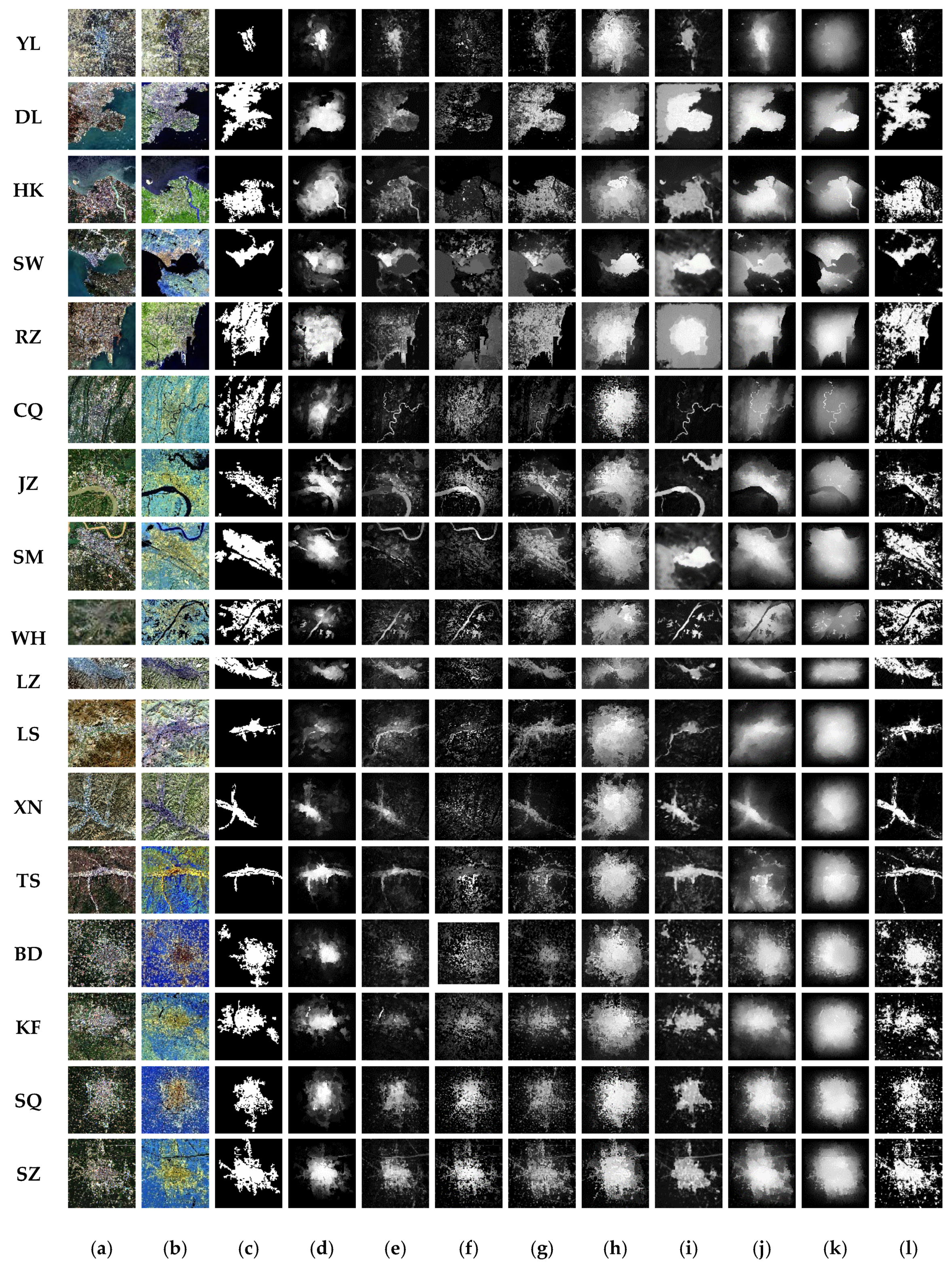
3.1. Comparison to the State-of-the-Art Saliency Methods
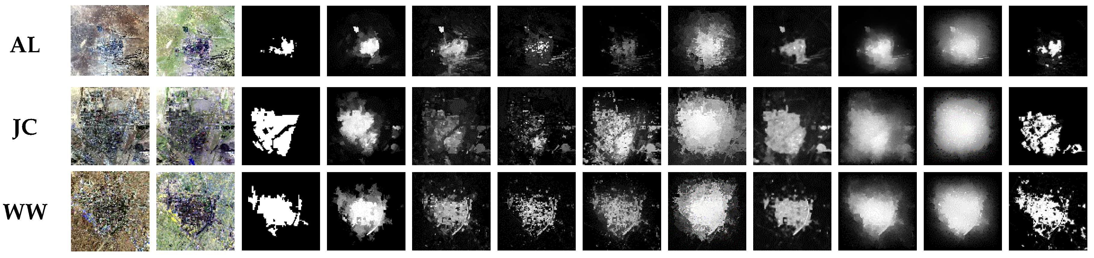
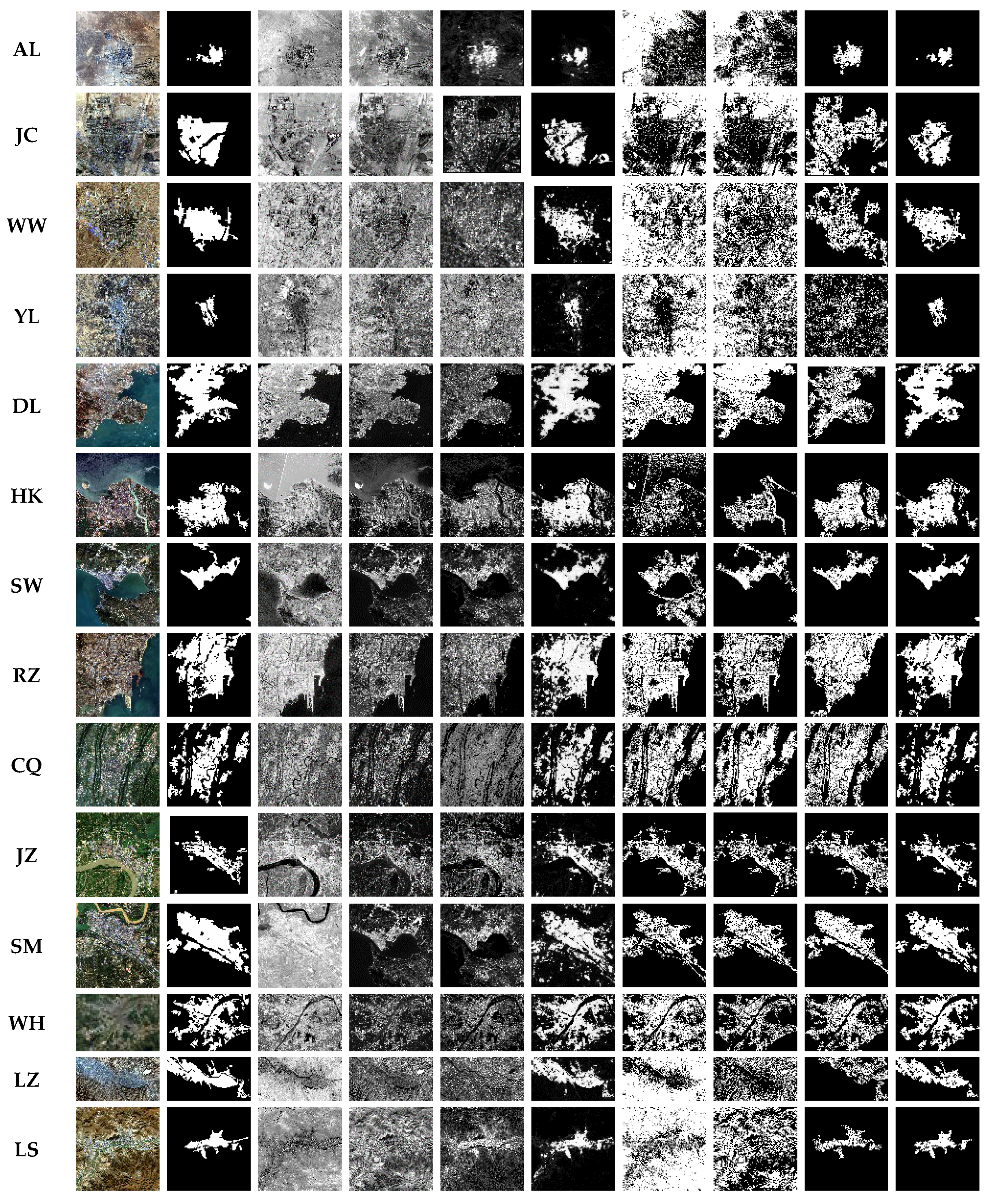
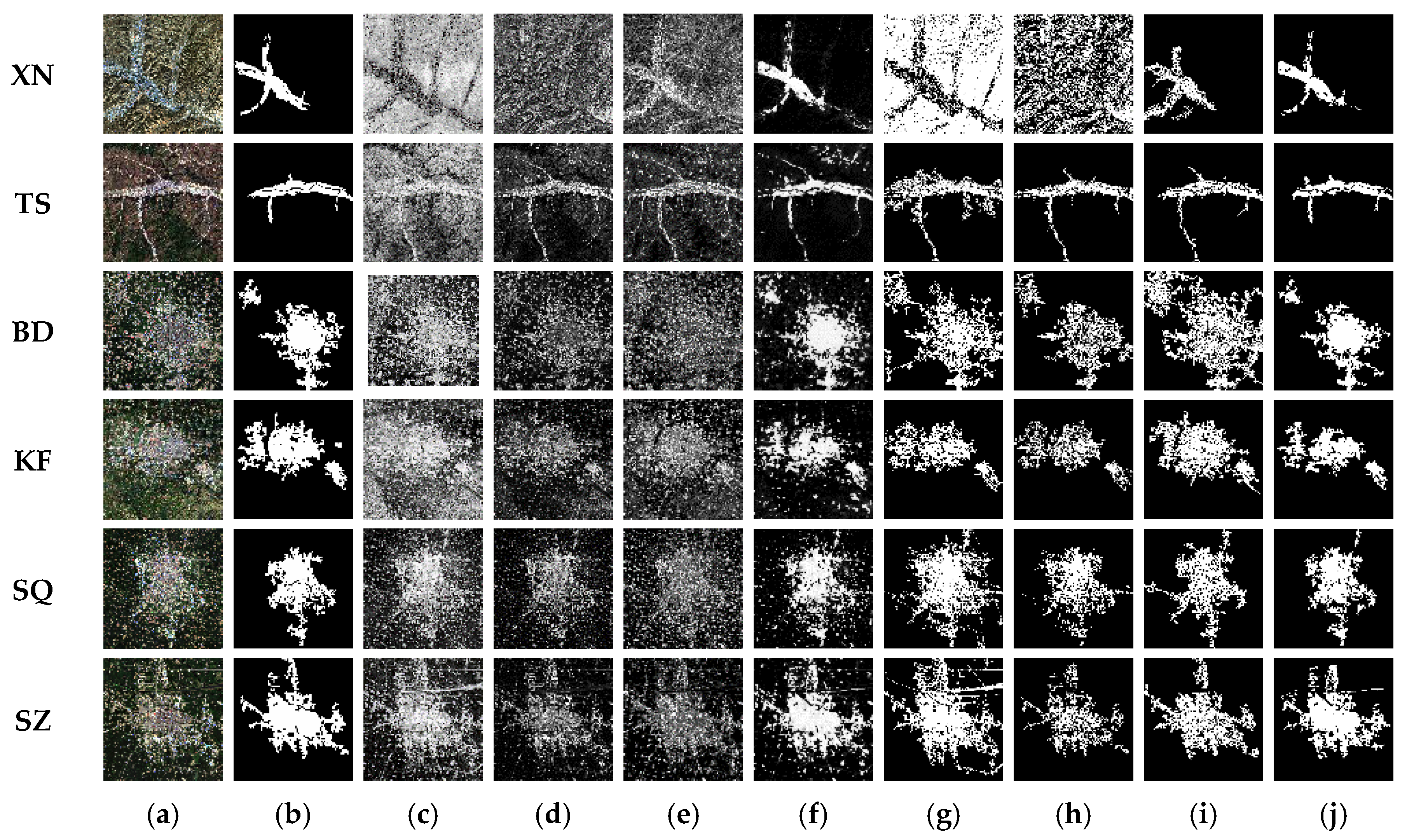
3.1.1. Qualitative Experiment
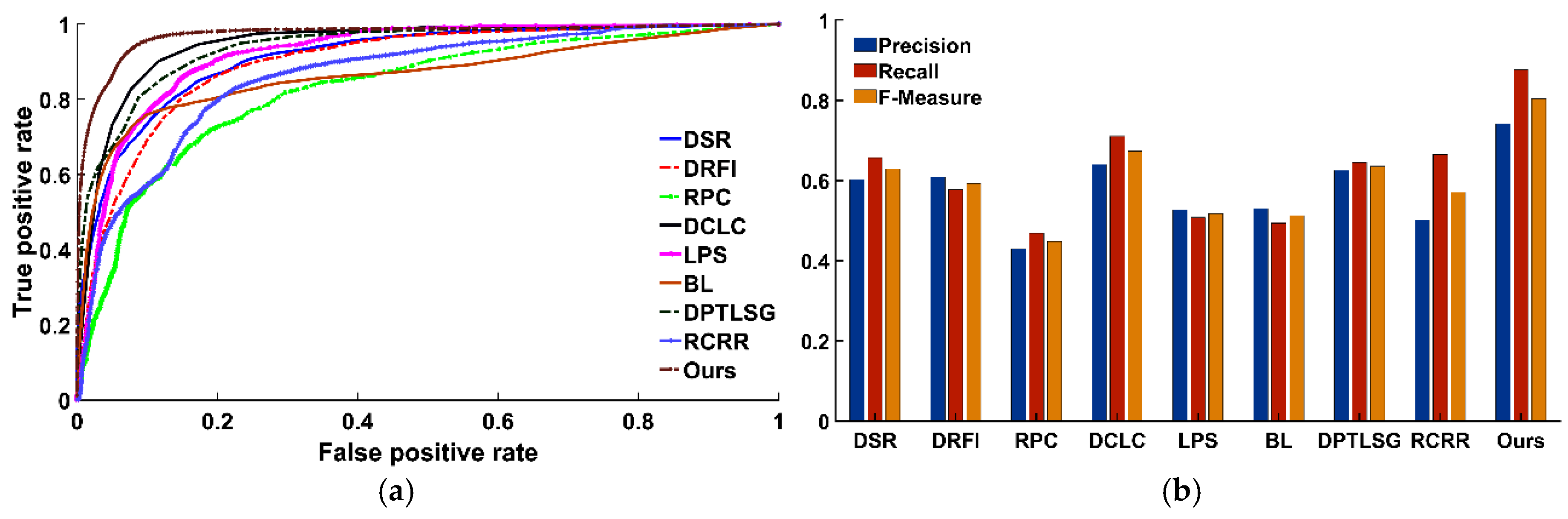
3.1.2. Quantitative Experiment
ROC-AUC Metric
Precision, Recall, and F-Measure
Time Comparison
3.1.3. Important Parameter Settings
3.2. Comparison to the State-of-the-Art Built-Up Areas Extraction Methods
4. Discussion
5. Conclusions
Author Contributions
Funding
Acknowledgments
Conflicts of Interest
References
- Taubenböck, H.; Esch, T.; Felbier, A.; Wiesner, M.; Roth, A.; Dech, S. Monitoring urbanization in mega cities from space. Remote Sens. Environ. 2012, 117, 162–176. [Google Scholar] [CrossRef]
- Yu, S.; Sun, Z.; Guo, H.; Zhao, X.; Sun, L.; Wu, M. Monitoring and analyzing the spatial dynamics and patterns of megacities along the maritime silk road. J. Remote Sens. 2017, 21, 169–181. [Google Scholar]
- Sun, Z.; Guo, H.; Li, X.; Lu, L.; Du, X. Estimating urban impervious surfaces from landsat-5 tm imagery using multilayer perceptron neural network and support vector machine. J. Appl. Remote Sens. 2011, 5, 053501. [Google Scholar] [CrossRef]
- Deng, C.; Wu, C. Bci: A biophysical composition index for remote sensing of urban environments. Remote Sens. Environ. 2012, 127, 247–259. [Google Scholar] [CrossRef]
- Jieli, C.; Manchun, L.; Yongxue, L.; Chenglei, S.; Wei, H.U. Extract residential areas automatically by new built-up index. In Proceedings of the 18th International Conference on Geoinformatics, Beijing, China, 18–20 June 2010. [Google Scholar]
- Xu, H. A new index for delineating built-up land features in satellite imagery. Int. J. Remote Sens. 2008, 29, 4269–4276. [Google Scholar] [CrossRef]
- Zha, Y.; Gao, J.; Ni, S. Use of normalized difference built-up index in automatically mapping urban areas from tm imagery. Int. J. Remote Sens. 2003, 24, 583–594. [Google Scholar] [CrossRef]
- Sun, G.; Chen, X.; Jia, X.; Yao, Y.; Wang, Z. Combinational build-up index (cbi) for effective impervious surface mapping in urban areas. IEEE J. Sel. Top. Appl. Earth Obs. Remote Sens. 2016, 9, 2081–2092. [Google Scholar] [CrossRef]
- Zhang, P.; Sun, Q.; Liu, M.; Li, J.; Sun, D. A strategy of rapid extraction of built-up area using multi-seasonal landsat-8 thermal infrared band 10 images. Remote Sens. 2017, 9, 1126. [Google Scholar] [CrossRef]
- Shao, Z.; Tian, Y.; Shen, X. Basi: A new index to extract built-up areas from high-resolution remote sensing images by visual attention model. Remote Sens. Lett. 2014, 5, 305–314. [Google Scholar] [CrossRef]
- Pesaresi, M.; Gerhardinger, A.; Kayitakire, F. A robust built-up area presence index by anisotropic rotation-invariant textural measure. IEEE J. Sel. Top. Appl. Earth Obs. Remote Sens. 2008, 1, 180–192. [Google Scholar] [CrossRef]
- Wentz, E.A.; Stefanov, W.L.; Gries, C.; Hope, D. Land use and land cover mapping from diverse data sources for an arid urban environments. Comput. Environ. Urban Syst. 2006, 30, 320–346. [Google Scholar] [CrossRef]
- Leinenkugel, P.; Esch, T.; Kuenzer, C. Settlement detection and impervious surface estimation in the mekong delta using optical and sar remote sensing data. Remote Sens. Environ. 2011, 115, 3007–3019. [Google Scholar] [CrossRef]
- Zhu, Z.; Woodcock, C.E.; Rogan, J.; Kellndorfer, J. Assessment of spectral, polarimetric, temporal, and spatial dimensions for urban and peri-urban land cover classification using landsat and sar data. Remote Sens. Environ. 2012, 117, 72–82. [Google Scholar] [CrossRef]
- Zhang, J.; Li, P.; Wang, J. Urban built-up area extraction from landsat tm/etm+ images using spectral information and multivariate texture. Remote Sens. 2014, 6, 7339–7359. [Google Scholar] [CrossRef]
- Borji, A.; Cheng, M.; Jiang, H.; Li, J. Salient object detection: A benchmark. IEEE Trans. Imag. Process. 2015, 24, 5706–5722. [Google Scholar] [CrossRef] [PubMed]
- Dong, C.; Liu, J.; Xu, F. Ship detection in optical remote sensing images based on saliency and a rotation-invariant descriptor. Remote Sens. 2018, 10, 400. [Google Scholar] [CrossRef]
- Zhang, Y.; Wang, X.; Xie, X.; Li, Y. Salient object detection via recursive sparse representation. Remote Sens. 2018, 10, 652. [Google Scholar] [CrossRef]
- Zhang, L.; Li, A.; Zhang, Z.; Yang, K. Global and local saliency analysis for the extraction of residential areas in high-spatial-resolution remote sensing image. IEEE Trans. Geosci. Remote Sens. 2016, 54, 3750–3763. [Google Scholar] [CrossRef]
- Itti, L.; Koch, C.; Niebur, E. A model of saliency-based visual attention for rapid scene analysis. IEEE Trans. Pattern Anal. Mach. Intell. 1998, 20, 1254–1259. [Google Scholar] [CrossRef] [Green Version]
- Harel, J.; Koch, C.; Perona, P. Graph-based visual saliency. In Advances in Neural Information Processing Systems; Touretzky, D.S., Mozer, M.C., Hasselmo, M.E., Eds.; MIT Press: Cambridge, MA, USA, 2007. [Google Scholar]
- Ma, Y.; Zhang, H. Contrast-based image attention analysis by using fuzzy growing. In Proceedings of the Eleventh ACM International Conference on Multimedia, Berkeley, CA, USA, 2–8 November 2003. [Google Scholar]
- Gao, D.; Mahadevan, V.; Vasconcelos, N. The discriminant center-surround hypothesis for bottom-up saliency. In Advances in Neural Information Processing Systems; Platt, J.C., Koller, D., Singer, Y., Roweis, S.T., Eds.; Curran Associates Icn: Vancouver, BC, Canada, 2008. [Google Scholar]
- Gao, D.; Vasconcelos, N. Bottom-up saliency is a discriminant process. In Proceedings of the 2007 IEEE 11th International Conference on Computer Vision, Rio de Janeiro, Brazil, 14–21 October 2007. [Google Scholar]
- Cheng, M.; Mitra, N.J.; Huang, X.; Torr, P.H.; Hu, S.-M.; Intelligence, M. Global contrast based salient region detection. IEEE Trans. Pattern Anal. Mach. Intell. 2015, 37, 569–582. [Google Scholar] [CrossRef] [PubMed]
- Perazzi, F.; Krähenbühl, P.; Pritch, Y.; Hornung, A. Saliency filters: Contrast based filtering for salient region detection. In Proceedings of the 2012 IEEE Conference on Computer Vision and Pattern Recognition, Providence, RI, USA, 16–21 June 2012. [Google Scholar]
- Shi, K.; Wang, K.; Lu, J.; Lin, L. Pisa: Pixelwise image saliency by aggregating complementary appearance contrast measures with spatial priors. In Proceedings of the 2013 IEEE Conference on Computer Vision and Pattern Recognition, Portland, OR, USA, 25–27 June 2013. [Google Scholar]
- Gopalakrishnan, V.; Hu, Y.; Rajan, D. Random walks on graphs for salient object detection in images. IEEE Trans. Imag. Process. 2010, 19, 3232–3242. [Google Scholar] [CrossRef] [PubMed]
- Wei, Y.; Wen, F.; Zhu, W.; Sun, J. Geodesic saliency using background priors. In Proceedings of the European Conference on Computer Vision, Florence, Italy, 7–13 October 2012. [Google Scholar]
- Jiang, B.; Zhang, L.; Lu, H.; Yang, C.; Yang, M.-H. Saliency detection via absorbing markov chain. In Proceedings of the 2013 IEEE International Conference on Computer Vision, Sydney, Australia, 3–6 December 2013. [Google Scholar]
- Yan, Q.; Xu, L.; Shi, J.; Jia, J. Hierarchical saliency detection. In Proceedings of the 2013 IEEE Conference on Computer Vision and Pattern Recognition, Oregon, Portland, 25–27 June 2013. [Google Scholar]
- Qin, Y.; Lu, H.; Xu, Y.; Wang, H. Saliency detection via cellular automata. In Proceedings of the 2015 IEEE Conference on Computer Vision and Pattern Recognition (CVPR), Boston, MA, USA, 8–10 June 2015. [Google Scholar]
- Bruce, N.; Tsotsos, J. Saliency based on information maximization. In Advances in Neural Information Processing Systems; Jordan, M.I., LeCun, Y., Solla, S.A., Eds.; MIT Press: Cambridge, MA, USA, 2006; pp. 155–162. [Google Scholar]
- Zhang, L.; Tong, M.H.; Marks, T.K.; Shan, H.; Cottrell, G.W. Sun: A bayesian framework for saliency using natural statistics. J. Vis. 2008, 8, 32. [Google Scholar] [CrossRef] [PubMed]
- Shen, X.; Wu, Y. A unified approach to salient object detection via low rank matrix recovery. In Proceedings of the 2012 IEEE Conference on Computer Vision and Pattern Recognition, Providence, RI, USA, 18–20 June 2012. [Google Scholar]
- Borji, A.; Itti, L. Exploiting local and global patch rarities for saliency detection. In Proceedings of the 2012 IEEE Conference on Computer Vision and Pattern Recognition, Providence, RI, USA, 18–20 June 2012. [Google Scholar]
- Wang, Q.; Zheng, W.; Piramuthu, R. Grab: Visual saliency via novel graph model and background priors. In Proceedings of the 2016 IEEE Conference on Computer Vision and Pattern Recognition (CVPR), Las Vegas, NV, USA, 26 June–1 July 2016. [Google Scholar]
- Zhu, W.; Liang, S.; Wei, Y.; Sun, J. Saliency optimization from robust background detection. In Proceedings of the 2014 IEEE Conference on Computer Vision and Pattern Recognition, Columbus, OH, USA, 24–27 June 2014. [Google Scholar]
- Peng, H.; Li, B.; Ji, R.; Hu, W.; Xiong, W.; Lang, C. Salient object detection via low-rank and structured sparse matrix decomposition. IEEE Trans. Patt. Anal. Mach. Intell. 2013, 39, 796–802. [Google Scholar]
- Lang, C.; Liu, G.; Yu, J.; Yan, S. Saliency detection by multitask sparsity pursuit. IEEE Trans. Imag. Process. 2012, 21, 1327–1338. [Google Scholar] [CrossRef] [PubMed]
- Jiang, H.; Wang, J.; Yuan, Z.; Wu, Y.; Zheng, N.; Li, S. Salient object detection: A discriminative regional feature integration approach. In Proceedings of the 2013 IEEE Conference on Computer Vision and Pattern Recognition, Oregon, Portland, 25–27 June 2013. [Google Scholar]
- Yang, J.; Yang, M. Top-down visual saliency via joint crf and dictionary learning. IEEE Trans. Patt. Anal. Mach. Intell. 2017, 39, 576–588. [Google Scholar] [CrossRef] [PubMed]
- Cholakkal, H.; Rajan, D.; Johnson, J. Top-Down Saliency with Locality-Constrained Contextual Sparse Coding. Available online: http://www.bmva.org/bmvc/2015/papers/paper159/paper159.pdf (accessed on 4 August 2018).
- Tong, N.; Lu, H.; Ruan, X.; Yang, M.-H. Salient object detection via bootstrap learning. In Proceedings of the 2015 IEEE Conference on Computer Vision and Pattern Recognition (CVPR), Boston, MA, USA, 8–10 June 2015. [Google Scholar]
- Wang, X.; Ma, H.; Chen, X. Geodesic weighted bayesian model for salient object detection. In Proceedings of the 2015 IEEE International Conference on Image Processing (ICIP), Quebec City, QC, Canada, 27–30 September 2015; pp. 397–401. [Google Scholar]
- Qin, Y.; Feng, M.; Lu, H.; Cottrell, G.W. Hierarchical cellular automata for visual saliency. Int. J. Comput. Vis. 2018, 1–20. [Google Scholar] [CrossRef]
- Couceiro, M.; Ghamisi, P. Fractional Order Darwinian Particle Swarm Optimization: Applications and Evaluation of an Evolutionary Algorithm; Springer: Berlin, Germany, 2015. [Google Scholar]
- Drusch, M.; Del Bello, U.; Carlier, S.; Colin, O.; Fernandez, V.; Gascon, F.; Hoersch, B.; Isola, C.; Laberinti, P.; Martimort, P. Sentinel-2: Esa’s optical high-resolution mission for gmes operational services. Remote Sens. Environ. 2012, 120, 25–36. [Google Scholar] [CrossRef]
- Vuolo, F.; Żółtak, M.; Pipitone, C.; Zappa, L.; Wenng, H.; Immitzer, M.; Weiss, M.; Baret, F.; Atzberger, C. Data service platform for sentinel-2 surface reflectance and value-added products: System use and examples. Remote Sens. 2016, 8, 938. [Google Scholar] [CrossRef]
- Mueller-Wilm, U. Sentinel-2 msi—Level-2a Prototype Processor Installation and User Manual. Available online: http://step.esa.int/thirdparties/sen2cor/2.2.1/S2PAD-VEGA-SUM-0001-2.2.pdf (accessed on 6 July 2018).
- Park, H.; Choi, J.; Park, N.; Choi, S. Sharpening the vnir and swir bands of sentinel-2a imagery through modified selected and synthesized band schemes. Remote Sens. 2017, 9, 1080. [Google Scholar] [CrossRef]
- Valdiviezo-N, J.C.; Téllez-Quiñones, A.; Salazar-Garibay, A.; López-Caloca, A.A. Built-up index methods and their applications for urban extraction from sentinel 2a satellite data: Discussion. J. Opt. Soc. Am. A 2018, 35, 35–44. [Google Scholar] [CrossRef] [PubMed]
- Pesaresi, M.; Corbane, C.; Julea, A.; Florczyk, A.J.; Syrris, V.; Soille, P.; Sensing, R. Assessment of the added-value of sentinel-2 for detecting built-up areas. Remote Sens. 2016, 8, 299. [Google Scholar] [CrossRef] [Green Version]
- Chavez, P.; Berlin, G.L.; Sowers, L.B. Statistical method for selecting landsat mss ratios. J. Appl. Photogr. Eng. 1982, 8, 23–30. [Google Scholar]
- Richards, J.A.; Richards, J. Remote Sensing Digital Image Analysis; Springer: Berlin, Germany, 1999. [Google Scholar]
- Swain, P.H.; Davis, S.M. Remote sensing: The quantitative approach. IEEE Trans. Patt. Anal. Mach. Intell. 1981, 713–714. [Google Scholar] [CrossRef]
- Achanta, R.; Shaji, A.; Smith, K.; Lucchi, A.; Fua, P.; Süsstrunk, S. Slic superpixels compared to state-of-the-art superpixel methods. IEEE Trans. Patt. Anal. Mach. Intell. 2012, 34, 2274–2282. [Google Scholar] [CrossRef] [PubMed]
- Moya, M.M.; Koch, M.W.; Perkins, D.N.; West, R.D.D. Superpixel segmentation using multiple sar image products. In Radar Sensor Technology XVIII; International Society for Optics and Photonics: Bellingham, WA, USA, 2014; p. 90770R. [Google Scholar]
- Hu, Z.; Wu, Z.; Zhang, Q.; Fan, Q.; Xu, J. A spatially-constrained color–texture model for hierarchical vhr image segmentation. IEEE Geosci. Remote Sens. Lett. 2013, 10, 120–124. [Google Scholar] [CrossRef]
- Connolly, C.; Fleiss, T. A study of efficiency and accuracy in the transformation from rgb to cielab color space. IEEE Trans. Imag. Process. 1997, 6, 1046–1048. [Google Scholar] [CrossRef] [PubMed]
- Hu, P.; Wang, W.; Zhang, C.; Lu, K. Detecting salient objects via color and texture compactness hypotheses. IEEE Trans. Imag. Process. 2016, 25, 4653–4664. [Google Scholar] [CrossRef] [PubMed]
- Ojala, T.; Pietikainen, M.; Maenpaa, T. Multiresolution gray-scale and rotation invariant texture classification with local binary patterns. IEEE Trans. Patt. Anal. Mach. Intell. 2002, 24, 971–987. [Google Scholar] [CrossRef] [Green Version]
- Jia, S.; Deng, B.; Zhu, J.; Jia, X.; Li, Q. Local binary pattern-based hyperspectral image classification with superpixel guidance. IEEE Trans. Geosci. Remote Sens. 2018, 56, 749–759. [Google Scholar] [CrossRef]
- Zhou, L.; Yang, Z.; Yuan, Q.; Zhou, Z.; Hu, D. Salient region detection via integrating diffusion-based compactness and local contrast. IEEE Trans. Imag. Process. 2015, 24, 3308–3320. [Google Scholar] [CrossRef] [PubMed]
- Zhou, D.; Weston, J.; Gretton, A.; Bousquet, O.; Schölkopf, B. Ranking on data manifolds. In Advances in Neural Information Processing Systems; Mit Press: Cambridge, MA, USA, 2004; pp. 169–176. [Google Scholar]
- Qiao, C.; Wang, J.; Shang, J.; Daneshfar, B. Spatial relationship-assisted classification from high-resolution remote sensing imagery. Int. J. Dig. Earth 2015, 8, 710–726. [Google Scholar] [CrossRef]
- Xie, Y.; Lu, H.; Yang, M. Bayesian saliency via low and mid level cues. IEEE Trans. Imag. Process. 2013, 22, 1689–1698. [Google Scholar]
- Boykov, Y.; Kolmogorov, V. An experimental comparison of min-cut/max-flow algorithms for energy minimization in vision. IEEE Trans. Patt. Anal. Mach. Intell. 2004, 26, 1124–1137. [Google Scholar] [CrossRef] [PubMed]
- Xu, H. Modification of normalised difference water index (ndwi) to enhance open water features in remotely sensed imagery. Int. J. Remote Sens. 2006, 27, 3025–3033. [Google Scholar] [CrossRef]
- Lu, H.; Zhang, X.; Qi, J.; Tong, N.; Ruan, X.; Yang, M.-H. Co-bootstrapping saliency. IEEE Trans. Imag. Process. 2017, 26, 414–425. [Google Scholar] [CrossRef] [PubMed]
- He, K.; Sun, J.; Tang, X. Guided image filtering. IEEE Trans. Patt. Anal. Mach. Intell. 2013, 1397–1409. [Google Scholar] [CrossRef] [PubMed]
- Li, K.; Chen, Y. A genetic algorithm-based urban cluster automatic threshold method by combining viirs dnb, ndvi, and ndbi to monitor urbanization. Remote Sens. 2018, 10, 277. [Google Scholar] [CrossRef]
- Li, X.; Lu, H.; Zhang, L.; Ruan, X.; Yang, M.-H. Saliency detection via dense and sparse reconstruction. In Proceedings of the 2013 IEEE International Conference on Computer Vision, Sydney, Australia, 1–8 December 2013. [Google Scholar]
- Lou, J.; Ren, M.; Wang, H. Regional principal color based saliency detection. PLoS ONE 2014, 9, e112475. [Google Scholar] [CrossRef] [PubMed]
- Li, H.; Lu, H.; Lin, Z.; Shen, X.; Price, B. Inner and inter label propagation: Salient object detection in the wild. IEEE Trans. Imag. Process. 2015, 24, 3176–3186. [Google Scholar] [CrossRef] [PubMed]
- Zhou, L.; Yang, Z.; Zhou, Z.; Hu, D. Salient region detection using diffusion process on a two-layer sparse graph. IEEE Trans. Imag. Process. 2017, 26, 5882–5894. [Google Scholar] [CrossRef] [PubMed]
- Yuan, Y.; Li, C.; Kim, J.; Cai, W.; Feng, D.D. Reversion correction and regularized random walk ranking for saliency detection. IEEE Trans. Imag. Process. 2018, 27, 1311–1322. [Google Scholar] [CrossRef] [PubMed]
- Pesaresi, M.; Huadong, G.; Blaes, X.; Ehrlich, D.; Ferri, S.; Gueguen, L.; Halkia, M.; Kauffmann, M.; Kemper, T.; Lu, L. A global human settlement layer from optical hr/vhr rs data: Concept and first results. IEEE J. Sel. Top. Appl. Earth Obs. Remote Sens. 2013, 6, 2102–2131. [Google Scholar] [CrossRef]
- Zhang, L.; Lv, X.; Liang, X. Saliency analysis via hyperparameter sparse representation and energy distribution optimization for remote sensing images. Remote Sens. 2017, 9, 636. [Google Scholar] [CrossRef]


| Start |
|---|
| Set Initial parameters vn [0], xn [0], χ1n [0], χ2n [0] // vn is position parameter, xn is velocity parameter, χ1n is local best, χ2n is global best |
| for i = 1:1:Max. Number of the iteration |
| Generated swarm matrix |
| for n = 1:1:Number of swarm matrix row |
| Calculate fitness function of each row |
| end |
| Obtain min. fitness function’s parameter configuration |
| If min. fitness function(i)<min. fitness function (i−1) |
| Update [t], [t] |
| Update [t + 1], [t + 1] |
| else |
| Kill all swarm matrix member |
| Go to “generated swarm matrix” |
| end |
| end |
| end |
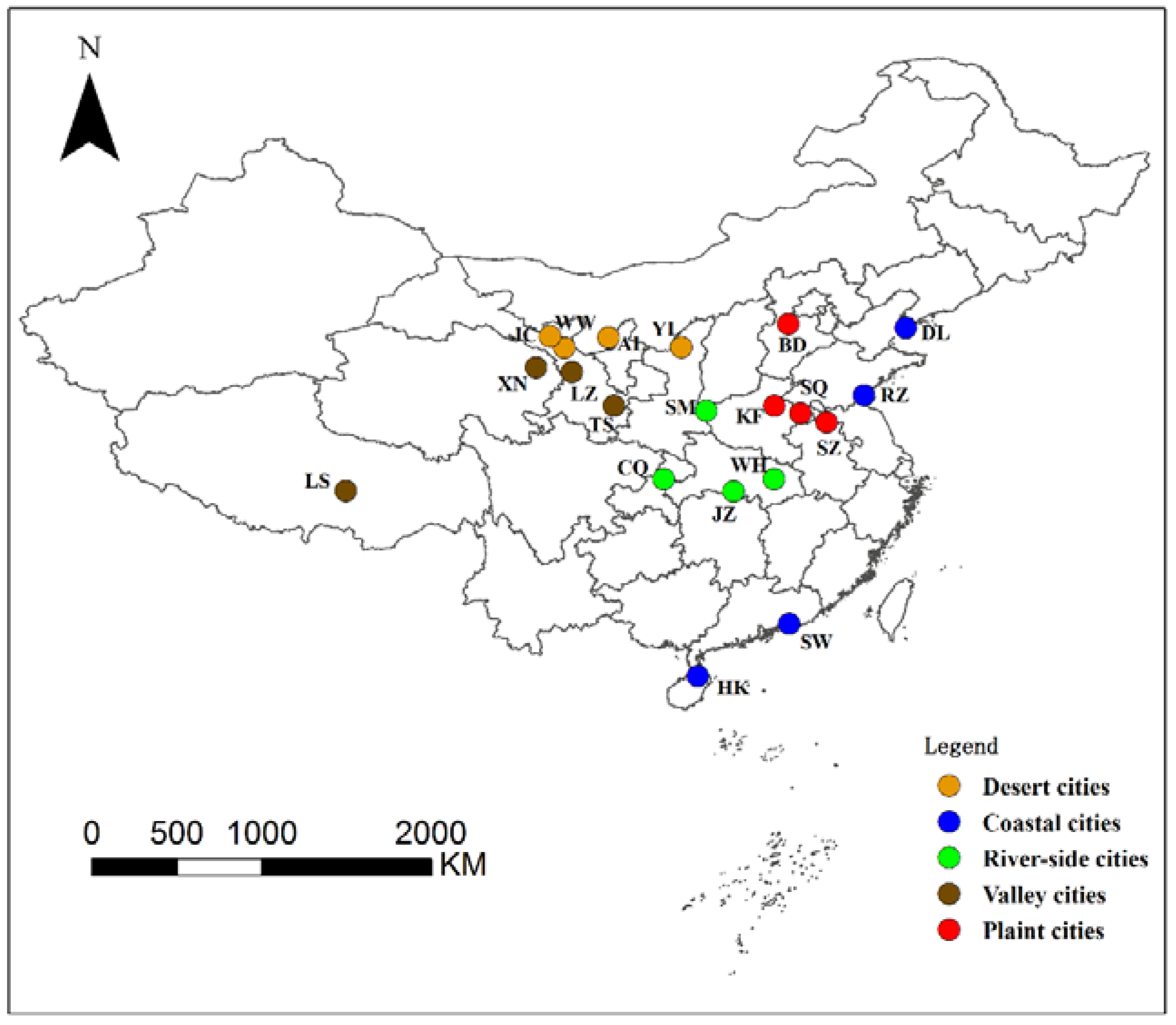
| City Type | City | Size (pixels) | Date |
|---|---|---|---|
| Desert cities | Alxa (Inner Mongolia) | 1000 × 900 | 11/01/2016 |
| Jinchang (Gansu) | 858 × 858 | 11/24/2016 | |
| Wuwei (Gansu) | 1000 × 1000 | 11/04/2016 | |
| Yulin (Shanxi) | 1500 × 1500 | 04/01/2016 | |
| Coastal cities | Dalian (Liaoning) | 1300 × 1300 | 11/21/2016 |
| Haikou (Hainan) | 1250 × 1250 | 12/20/2016 | |
| Rizhao (Shandong) | 1000 × 1000 | 11/03/2016 | |
| Shanwei (Guangdong) | 500 × 500 | 12/13/2016 | |
| Riverside cities | Chongqing | 1650 × 1650 | 04/14/2017 |
| Jinzhou (Hubei) | 1250 × 1250 | 08/01/2016 | |
| Sanmenxia (Henan) | 1000 × 1000 | 09/23/2016 | |
| Wuhan (Hubei) | 1800 × 1200 | 08/28/2016 | |
| Valley cities | Lanzhou (Gansu) | 1750 × 900 | 12/01/2016 |
| Lhasa (Tibet) | 1500 × 1500 | 10/24/2016 | |
| Tianshui (Gansu) | 1020 × 1020 | 06/06/2017 | |
| Xining (Qinghai) | 1750 × 1750 | 11/04/2016 | |
| Plain cities | Baoding (Hebei) | 1400 × 1400 | 09/01/2016 |
| Kaifeng (Henan) | 1200 × 1200 | 08/23/2016 | |
| Shangqiu (Henan) | 1250 × 1250 | 08/28/2016 | |
| Suzhou (Anhui) | 1200 × 1200 | 08/28/2016 |
| Desert City | Cities | Alxa | Jinchang | Wuwei | Yulin |
| Optimal | Bands 12, 11, 7 | Bands 12, 11, 7 | Bands 12, 11, 5 | Bands 12, 11, 7 | |
| Coastal City | Cities | Dalian | Haikou | Shanwei | Rizhao |
| Optimal | Bands 12, 11, 7 | Bands 12, 11, 7 | Bands 12, 11, 7 | Bands 12, 11, 5 | |
| Riverside Cities | Cities | Chongqing | Jingzhou | Sanmenxia | Wuhan |
| Optimal | Bands 12, 11, 7 | Bands 12, 11, 7 | Bands 12, 11, 7 | Bands 12, 11, 7 | |
| Valley Cities | Cities | Lanzhou | Lhasa | Tianshui | Xining |
| Optimal | Bands 12, 11, 5 | Bands 12, 11, 5 | Bands 12, 11, 5 | Bands 12, 11, 7 | |
| Plain Cities | Cities | Baoding | Kaifeng | Shangqing | Suzhou |
| Optimal | Bands 12, 11, 7 | Bands 12, 11, 7 | Bands 12, 11, 7 | Bands 12, 11, 7 |
| Method | DSR | DRFI | RPC | DCLC | LPS | BL | DPTLSG | RCRR | Ours | ||
|---|---|---|---|---|---|---|---|---|---|---|---|
| AUC | 0.8890 | 0.8788 | 0.7521 | 0.9146 | 0.8485 | 0.8366 | 0.9167 | 0.8405 | 0.9687 | ||
| Method | DSR | DRFI | RPC | DCLC | LPS | BL | DPTLSG | RCRR | Ours |
|---|---|---|---|---|---|---|---|---|---|
| Time(s) | 178.33 | 1547.65 | 514.23 | 325.42 | 137.92 | 135.24 | 1583.00 | 1363.15 | 1226.22 |
| M | M = 3 (N = 1000, 1500, 2000) | M = 5 (N = 1000, 1500, 2000, 2500, 3000) | M = 7 (N = 1000, 1500, 2000, 2500, 3000, 3500, 4000) |
|---|---|---|---|
| AUC | 0.9645 | 0.9664 | 0.9687 |
| F-Measure | 0.7853 | 0.7868 | 0.8038 |
| Time(s) | 259.60 | 626.42 | 1226.22 |
| ϑ | 1.2 | 1.4 | 1.6 | 1.8 | 2.0 |
|---|---|---|---|---|---|
| AUC | 0.9534 | 0.9581 | 0.9592 | 0.9597 | 0.9487 |
| F-Measure | 0.7147 | 0.7212 | 0.7299 | 0.7378 | 0.7148 |
| NDBI | NBI | PanTex | Ours | |||||||||
|---|---|---|---|---|---|---|---|---|---|---|---|---|
| OA | Co | Om | OA | Co | Om | OA | Co | Om | OA | Co | Om | |
| Desert | 36.40 | 90.85 | 65.66 | 42.52 | 90.48 | 64.32 | 81.27 | 65.18 | 33.87 | 95.56 | 11.25 | 26.26 |
| Costal | 78.22 | 48.27 | 30.59 | 86.06 | 27.66 | 27.18 | 87.88 | 36.66 | 36.39 | 95.13 | 8.04 | 11.17 |
| Riverside | 80.96 | 38.64 | 24.07 | 84.51 | 29.34 | 28.92 | 81.57 | 37.21 | 29.03 | 93.35 | 10.49 | 17.84 |
| Valley | 48.62 | 83.01 | 48.86 | 64.62 | 71.72 | 43.35 | 87.81 | 29.54 | 25.91 | 96.37 | 11.68 | 18.79 |
| Plain | 88.43 | 30.87 | 16.87 | 88.56 | 21.61 | 40.45 | 87.80 | 30.27 | 22.26 | 94.77 | 8.72 | 17.97 |
© 2018 by the authors. Licensee MDPI, Basel, Switzerland. This article is an open access article distributed under the terms and conditions of the Creative Commons Attribution (CC BY) license (http://creativecommons.org/licenses/by/4.0/).
Share and Cite
Sun, Z.; Meng, Q.; Zhai, W. An Improved Boosting Learning Saliency Method for Built-Up Areas Extraction in Sentinel-2 Images. Remote Sens. 2018, 10, 1863. https://doi.org/10.3390/rs10121863
Sun Z, Meng Q, Zhai W. An Improved Boosting Learning Saliency Method for Built-Up Areas Extraction in Sentinel-2 Images. Remote Sensing. 2018; 10(12):1863. https://doi.org/10.3390/rs10121863
Chicago/Turabian StyleSun, Zhenhui, Qingyan Meng, and Weifeng Zhai. 2018. "An Improved Boosting Learning Saliency Method for Built-Up Areas Extraction in Sentinel-2 Images" Remote Sensing 10, no. 12: 1863. https://doi.org/10.3390/rs10121863
APA StyleSun, Z., Meng, Q., & Zhai, W. (2018). An Improved Boosting Learning Saliency Method for Built-Up Areas Extraction in Sentinel-2 Images. Remote Sensing, 10(12), 1863. https://doi.org/10.3390/rs10121863