Neural Network Based Kalman Filters for the Spatio-Temporal Interpolation of Satellite-Derived Sea Surface Temperature

Abstract

The forecasting and reconstruction of oceanic dynamics is a crucial challenge. While model driven strategies are still the state-of-the-art approaches in the reconstruction of spatio-temporal dynamics. The ever increasing availability of data collections in oceanography raised the relevance of data-driven approaches as computationally efficient representations of spatio-temporal fields reconstruction. This tools proved to outperform classical state-of-the-art interpolation techniques such as optimal interpolation and DINEOF in the retrievement of fine scale structures while still been computationally efficient comparing to model based data assimilation schemes. However, coupling this data-driven priors to classical filtering schemes limits their potential representativity. From this point of view, the recent advances in machine learning and especially neural networks and deep learning can provide a new infrastructure for dynamical modeling and interpolation within a data-driven framework. In this work we adress this challenge and develop a novel Neural-Network-based (NN-based) Kalman filter for spatio-temporal interpolation of sea surface dynamics. Based on a data-driven probabilistic representation of spatio-temporal fields, our approach can be regarded as an alternative to classical filtering schemes such as the ensemble Kalman filters (EnKF) in data assimilation. Overall, the key features of the proposed approach are two-fold: (i) we propose a novel architecture for the stochastic representation of two dimensional (2D) geophysical dynamics based on a neural networks, (ii) we derive the associated parametric Kalman-like filtering scheme for a computationally-efficient spatio-temporal interpolation of Sea Surface Temperature (SST) fields. We illustrate the relevance of our contribution for an OSSE (Observing System Simulation Experiment) in a case-study region off South Africa. Our numerical experiments report significant improvements in terms of reconstruction performance compared with operational and state-of-the-art schemes (e.g., optimal interpolation, Empirical Orthogonal Function (EOF) based interpolation and analog data assimilation).

1. Introduction

The spatio-temporal high resolution monitoring of sea surface geophysical parameters (e.g., temperature, salinity, ocean colour) is of key interest for a variety of scientific fields [1,2,3]. Direct observations of these geophysical tracers are provided by satellite remote sensing observations and in-situ networks. However, due to sensors characteristics (e.g., space-time sampling, sensor type) and their sensitivity to the atmospheric conditions (e.g., rain, clouds), only partial, with potentially high missing data rates, and possibly noisy observations are available. As a consequence, providing high resolution gape free spatio-temporal fields, in both space and time, based on these observations have long been a crucial challenge that motivated the development of several spatio-temporal interpolation tools.

Within the satellite ocean community, Optimal Interpolation (OI) is a standard technique used in several operational products [4,5,6,7,8,9,10]. Given a covariance model of spatio-temporal dynamics, the interpolated field results from a linear combination of the observations. In general, stationary covariance hypotheses are considered, which prove relevant for the reconstruction of horizontal scales above 100 km. Fine scale components in the other hand may hardly be retrieved with such approaches and a variety of research studies aim to improve the reconstruction of high-resolution components of spatio-temporal fields.

Empirical Orthogonal Function (EOF) based interpolation is an other category widely used in geosciences [11,12,13]. It relies on a Singular Value Decomposition (SVD) to compute an EOF basis, the field is then reconstructed by projecting the observations on the EOF subspace until a convergence criterion is reached [14]. Unfortunately, dealing with high missing data rates decreases the encoded variability in the EOF components witch results in smoothing fine scale structures.

Data assimilation is the state-of-the-art framework for the reconstruction of dynamical systems from partial observations based on a given numerical model [15,16]. Statistical data assimilation schemes, especially ensemble Kalman filters, have become particularly popular due to their trade-off between computational efficiency and modeling flexibility. Unlike OI and EOF based techniques, these schemes explicitly rely on dynamical priors to address interpolation issues resulting in better representation of fine scale components. However, When dealing with sea surface dynamics, the analytical derivation of these priors involves simplifying assumptions which may not be satisfied by real observations [17]. By contrast, realistic analytical parameterizations may lead to highly computationally-demanding numerical models associated with modeling and inversion uncertainties [18], which may limit their relevance for an application of the interpolation of a single sea surface tracer.

Recently, data-driven approaches [11,19] have emerged as relevant alternatives to model-driven schemes. They take benefit from the increasing availability of remote sensing observations and simulation data to derive computationally efficient [20] dynamical priors. Analog methods are one of the first data-driven techniques developed within a data assimilation framework [19]. In our recent study [20,21,22], we proved the relevance of such data-driven approache when addressing the spatio-temporal interpolation of sea surface geophysical tracers. Combining analog data assimilation (AnDA) with a patch-based representation have shown great results with respect to the state-of-the-art OI and EOF-based schemes. However, the parametrization of the proposed framework involves tuning several parameters principally due to the data-driven formulation of the dynamical prior based on analog forecasting. The implementation of this dynamical prior in an ensemble filtering scheme also limits the representativity of the model as a trad-off between the method’s parameters and the ensemble size need to be addressed carefully to decrease the computational complexity of the assimilation method. From this point of view, several works [23,24] tried to formulate stochastic representations of dynamical operators for their optimal use in sequential filtering schemes. Methods based on prior knowledge of the variability of dynamical models have already been addressed to infer probabilistic representations. However, such techniques are limited to systems with available dynamical priors. Complex dynamical models in the other hand may require complex priors which may be unavailable or hard to derive.

In the last years, Neural Networks have enriched the state-of-the-art in probabilistic modelling. This is principally due to the advances in deep learning models which allow better understanding of complicated systems. Probabilistic representations such as structured inference [25] and deep Gaussian processes [26] have rapidly became very popular in applications such as generative modeling and dynamical inference. From this point of view the stochastic modelization of spatio-temporal fields is an interesting open challenge that may benefit from these advances and can allow the representation of complex stochastic dynamics without any prior knowledge regarding our system.

In this paper, we investigate data-driven interpolation approaches within a statistical data assimilation framework. We aim to derive stochastic data-driven representations of complex geophysical tracers. Among other representations [27] Neural networks are particularly appealing due to their efficient trad-off between modeling abilities and interpretability of the learnt models. This models have rapidly become the state-of-the-art in machine learning for a wide range of applications, including inverse imaging issues [28]. Recent applications to the assimilation of low-dimensional dynamical systems [27] and to the forecasting of geophysical dynamics [29,30] have been developed. However, to our knowledge, the design of neural-network-based assimilation models for the spatio-temporal interpolation of geophysical dynamics remain an open challenge, which may greatly benefit from the ability of deep learning models to capture computationally-efficient representations from available ocean observation and simulation datasets. In this study, we address this challenge and propose a novel NN-based Kalman filtering scheme applied to the spatio-temporal interpolation of satellite-derived sea surface temperature. We aim to propose a parametric data driven framework that embed a stochastic representation of spatio-temporal dynamics. this architecture conveys a probabilistic representation through the prediction of a mean component and a covariance pattern. The latter may be regarded as a NN-based representation of the covariance patterns issued from Monte Carlo approximations in ensemble assimilation schemes [31]. Our model may then be directly exploited in sequential filtering schemes which allows us to overcome both issues encountered in analog data assimilation and parametric stochastic representations based on prior knowledge in terms of numerical complexity and availability of dynamical priors. Overall, the methodological contributions of this work are two-fold: (i) we propose a new probabilistic NN-based representation of 2D geophysical dynamics, (ii) we derive the associated NN-based Kalman filtering scheme for spatio-temporal interpolation issues. We demonstrate the relevance of these contributions with respect to state-of-the-art approaches [5,11,22] for the spatio-temporal interpolation of satellite-derived SST fields in a case study region off South Africa. This region involves complex fine-scale SST dynamics (e.g., fronts, filaments) which can’t be retrieved using classical state-of-the-art techniques.

This paper is organized as follows. Section 2 reviews data assimilation schemes. Section 3 describes the proposed neural-network-based data assimilation framework. Section 4 presents the SST dataset used in our experiments as well as the parametrization chosen for the proposed model and benchmark techniques. Section 5 presents the results of the numerical experiments. We further discuss our contributions in Section 6.

2. Problem Statement and Related Work

Regarding ocean remote sensing data, spatio-temporal interpolation issues (also referred to as data assimilation in geoscience) can be regarded as the reconstruction of some hidden states from partial and/or noisy observation series [31]. Data assimilation techniques usually involve a state-space evolution model [31]:

$$\begin{array}{cc}\hfill x_{t+1}& =\mathcal{F}\left(x_t\right)+{\eta }_t\hfill \end{array}$$

(1)

$$\begin{array}{cc}\hfill y_{t+1}& =\mathcal{H}\left(x_{t+1}\right)+{ϵ}_t\hfill \end{array}$$

(2)

where $t\in \left\{0,\dots ,T\right\}$ represents the temporal resolution of our time series and $\mathcal{F}$ the dynamical model describing the temporal evolution of the physical variables x. The observation model $\mathcal{H}$ links the observation y to the physical variable x. ${\eta }_t$ and ${ϵ}_t$ are random processes accounting for the uncertainties in the dynamical and observation models. They are usually defined as centered Gaussian processes with covariances $Q_t$ and $R_t$ respectively.

From a probabilistic point of view, the spatio-temporal interpolation problem can be seen as a Bayesian filtering problem where the main goal is to evaluate the conditional probabilities $p\left(x_{t+1}\right|y_1,\dots ,y_t)$ (prediction distribution of the state $x_{t+1}$ given observations up to time t) and $p\left(x_{t+1}\right|y_1,\dots ,y_t,\dots ,y_{t+1})$ (posterior distribution of $x_{t+1}$ given observations up to time $t+1$). Under certain assumptions over the state space model (the dynamical and observation models are linear with Gaussian uncertainties), the prediction and posterior distributions are also Gaussian and can be written as:

$$\begin{array}{cc}\hfill p\left(x_{t+1}\right|y_1,\dots ,y_t)& =\mathcal{N}(x_{t+1}^{-},{\Sigma }_{t+1}^{-})\hfill \end{array}$$

(3)

$$\begin{array}{cc}\hfill p\left(x_{t+1}\right|y_1,\dots ,y_{t+1})& =\mathcal{N}(x_{t+1}^{+},{\Sigma }_{t+1}^{+})\hfill \end{array}$$

(4)

with the means and covariances computed for each time t using the well known Kalman recursion

$$\begin{array}{cc}\hfill x_{t+1}^{-}& =F{x}_t^{+}\hfill \end{array}$$

(5)

$$\begin{array}{cc}\hfill {\Sigma }_{t+1}^{-}& =F{\Sigma }_t^{+}{F}^T+Q_t\hfill \end{array}$$

(6)

$$\begin{array}{cc}\hfill x_{t+1}^{+}& =x_{t+1}^{-}+K_{t+1}[y_{t+1}-H_{t+1}{x}_{t+1}^{-}]\hfill \end{array}$$

(7)

$$\begin{array}{cc}\hfill {\Sigma }_{t+1}^{+}& ={\Sigma }_{t+1}^{-}-K_{t+1}{H}_{t+1}{\Sigma }_{t+1}^{-}\hfill \end{array}$$

(8)

with

$$\begin{array}{cc}\hfill K_{t+1}& ={\Sigma }_{t+1}^{-}{H}_{t+1}^T{[H_{t+1}{\Sigma }_{t+1}^{-}{H}_{t+1}^T+R_t]}^{-1}.\hfill \end{array}$$

(9)

Here F and $H_{t+1}$ corresponds respectively to some linear dynamical and observation models. The superscript (-) refers to the forecasting of the mean of the state variable $x_{t+1}^{-}$ and of its covariance matrix ${\Sigma }_{t+1}^{-}$ given observations up to time t but without the new observation at time $t+1$. The superscript (+) refers in the other hand to the mean of the state variable $x_{t+1}^{+}$ and of the covariance matrix ${\Sigma }_{t+1}^{+}$ given all observations up to time $t+1$. They are referred to as the assimilated mean and covariance. $K_{t+1}$ is the Kalman gain. Kalman filters provide a sequential formulation of the Optimal Interpolation (OI) [15] which may also be solved directly knowing the space-time covariance of processes x and y. For non-linear and high-dimensional dynamical systems, the Probability Density Functions (PDFs) are not Gaussian anymore and the above Kalman recursion does define their means and covariances. Ensemble Kalman methods have been proposed to address these issues. The ensemble Kalman filter and smoother [31] are the first sequential filtering techniques used reliably in the reconstruction of geophysical fields. The key idea here is to approximate the forecasting mean $x_{t+1}^{-}$ and covariance ${\Sigma }_{t+1}^{-}$ by a sample mean and covariance matrix computed by propagating an ensemble of M members, ${\{x_{t+1}^{i-}\}}_{i=1}^M$, using the dynamical model $\mathcal{F}$.

$$\begin{array}{cc}\hfill x_{t+1}^{i-}& =\mathcal{F}(x_t^{i+},i\in \left\{0,\dots ,N\right\})\hfill \end{array}$$

(10)

$$\begin{array}{cc}\hfill {\Sigma }_{t+1}^{-}& =\frac{1}{N-1}{D}_{t+1}{D}_{t+1}^t\hfill \end{array}$$

(11)

$$\begin{array}{cc}\hfill D_{t+1}& =[x_{t+1}^{1-}-x_{t+1}^{-},\dots x_{t+1}^{N-}-x_{t+1}^{-}]\hfill \end{array}$$

(12)

$$\begin{array}{cc}\hfill x_{t+1}^{i+}& =x_{t+1}^{i-}+K_{t+1}[y_{t+1}-H_{t+1}{x}_{t+1}^{i-}]\hfill \end{array}$$

(13)

$$\begin{array}{cc}\hfill K_{t+1}& ={\Sigma }_{t+1}^{-}{H}_{t+1}^T{[H_{t+1}{\Sigma }_{t+1}^{-}{H}_{t+1}^T+R_t]}^{-1}\hfill \end{array}$$

(14)

$$\begin{array}{cc}\hfill {\Sigma }_{t+1}^{+}& ={\Sigma }_{t+1}^{-}-K_{t+1}{H}_{t+1}{\Sigma }_{t+1}^{-}\hfill \end{array}$$

(15)

Besides all its advantages, EnKF techniques do not escape the curse of dimensionality. High-dimensional systems require using large ensemble sizes M which may lead to very high-computational complexity. The use of small ensemble sizes in the other hand may result in undersampling the covariance matrix (the considered ensemble is not representative of our systems dynamics) which may in turn result in poor reconstruction performance, including for instance filter divergence and spurious long-range correlations. Proposed solutions such as inflation [32], cross-validation [33] and localization methods [34,35,36] may require thorough tuning experiments. An alternative strategy based on a model-driven propagation of parametric covariance models  [23,24] seems appealing. Using advection priors [37], it propagates parametric covariance structures, which leads to the implementation of the classic Kalman recursion. Accounting for more complex dynamical priors for the covariance structure is an open question, which may limit the applicability of this approach to complex geophysical systems. Inspired by the latter parametric framework, we aim to design an efficient sequential filtering technique for the reconstruction of geophysical fields. Rather than considering a model-driven prior to propagate Gaussian states as in [23,24], we investigate NN-based priors, which may be fitted from training data. The resulting NN-based Gaussian representations provide computationally-efficient approximations of the dynamical priors that should prevent undersampling issues within a Kalman recursion.

3. Proposed Interpolation Model

3.1. Neural-Network Gaussian Dynamical Prior

Our key idea is to exploit neural-network (NN) representations for the time propagation of a Gaussian approximation of the distribution of the physical variable x. Compared with dynamical priors in the assimilation model (1), which states the conditional distribution $x_t|x_{t-1}$, we consider neural-network representations to extend the prediction step of the Kalman recursion (5) and (6) to non-linear dynamics. Formally, it comes to define:

$$x_{t+1}^{-}=\mathcal{F}\left(x_t^{+}\right)$$

(16)

$${\Sigma }_{t+1}^{-}={\mathcal{F}}_{\Sigma }(x_t^{+},{\Sigma }_t^{+})$$

(17)

with $x_{t+1}^{-}$ and ${\Sigma }_{t+1}^{-}$ the predicted mean and covariance of the Gaussian approximation of the state at time $t+1$ given the assimilated mean $x_t^{+}$ and covariance ${\Sigma }_t^{+}$ at time t. Functions $\mathcal{F},{\mathcal{F}}_{\Sigma }$ are neural networks to be defined with parameter vectors $\theta =({\theta }_{\mu },{\theta }_{\Sigma })$. It may be noted that our parameterization follows (5) and (6) such that the update of the mean component in (16) only depends on the mean at the previous time step and the update of the covariance depends both on the mean and covariance at the previous time step. Given this NN-based representation of the prediction step of the Kalman filter, we apply the classic Kalman-based filtering under the assumption that the observation model is linear and Gaussian.

Such a formulation does not require forecasting an ensemble to compute a sample covariance matrix. It results in a significant reduction of the computational complexity. The same holds when compared to the computational complexity of the analog data assimilation which involves ensemble forecasting and repeated nearest-neighbor search.

3.2. Patch-Based NN Architecture

When considering spatio-temporal fields, the application of the model defined by (16) and (17) should be considered with care to account for the underlying dimensionality, especially for the covariance model. For this reason, a global representation of the spatio-temporal field is most likely to fail due to computational limitations. Following our previous works on analog data assimilation [21,22], we consider a patch-based representation as sketched in Figure 1 (A patch is a $P\times P$ subregion of a 2D field with P the width and the height of the patch). This patch-based representation is fully embedded in the considered NN architecture to make explicit both the extraction of the patches from a 2D field and the reconstruction of a 2D field from the collection of patches. The latter involves a reconstruction operator which is learnt from data.

Regarding model $\mathcal{F}$, the proposed architecture proceeds as follows:

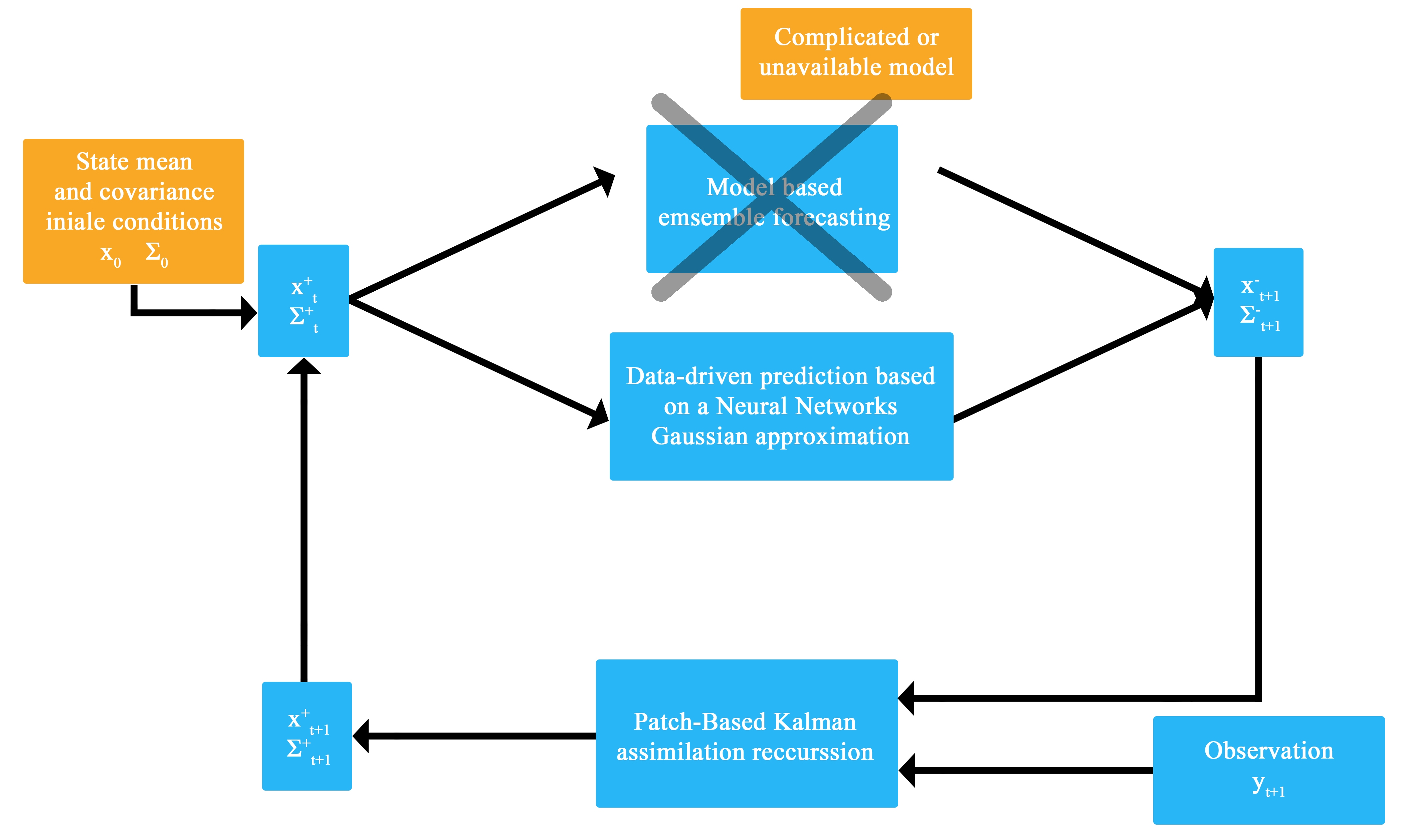
• At a given time t, the first layer of the network, which is parameter-free in terms of training, comes to decompose an input field $x_t$ into a collection of $N_p$ $P\times P$ patches $x_{{\mathcal{P}}_s,t}$, where P is the width and height of each patch and s the patch location in the global field. Each patch is decomposed onto an EOF basis $\mathcal{B}$ according to:

  $$\begin{array}{c}\hfill z_{{\mathcal{P}}_s,t}=x_{{\mathcal{P}}_s,t}{\mathcal{B}}^T\end{array}$$

  (18)

  with $z_{{\mathcal{P}}_s,t}$ the EOF decomposition of the patch $x_{{\mathcal{P}}_s,t}$. The EOF decomposition matrix $\mathcal{B}$ is trained offline as preprocessing step; For each $s\in [1,\dots ,N_p]$, we predict $z_{{\mathcal{P}}_s,t+1}$ using an EOF-patch-based model ${\mathcal{F}}^{{\mathcal{P}}_s}$. This model is implemented based on a residual architecture to mimic a numerical integration scheme (typically, an Euler or 4th-order Runge-Kutta scheme) of an approximate Ordinary Differential Equation (ODE) parametrized by the residual block of our residual network. By contrast to other neural networks models, This architecture grantee the physical interpretability of our dynamical model as stated in [27]. In order to enhance the modeling capabilities of our approximate model, The residual block is a classic Multilayer Perceptron (MLP) network with bilinear layers;
• The third layer is a reconstruction network ${\mathcal{F}}_r$. It combines the predicted patches $x_{{\mathcal{P}}_s,t}=z_{{\mathcal{P}}_s,t}\mathcal{B},s\in [1,\dots ,N_p]$ to reconstruct the output field $x_t$. This reconstruction network ${\mathcal{F}}_r$ involves a convolution neural network [38].

The details of the considered parameterizations for the second and third layers are given in Section 4. To train the mean dynamical model $\mathcal{F}$, we apply a two-step procedure. We first learn the local dynamical models ${\mathcal{F}}^{{\mathcal{P}}_s},s\in [1,\dots ,N_p]$ based on the minimization of the EOF-patch based forecasting error. The reconstruction network ${\mathcal{F}}_r$ is then optimized using the same criterion over the global field. This training procedure allows the patch based models to be interpreted as local dynamical models and the reconstruction network as a post-processing operator. Other training configurations could be envisaged, we can for example train the all model according to a forecasting error over the global field. However, this results in inconsistent patch models ${\mathcal{F}}^{{\mathcal{P}}_s}$ that can’t be used in assimilation experiments for patch reconstruction issues.

Regarding the covariance model ${\mathcal{F}}_{\Sigma }$, we also consider a patch-based representation of the spatial domain. More precisely, a block-diagonal parameterization of the covariance model ${\mathcal{F}}_{\Sigma }$ is addressed by training diagonal patch-level covariance models in the EOF space. It may be noted that a diagonal parameterization of the covariance in the EOF space forms a full covariance matrix in the original patch space.

Each patch based covariance model ${\mathcal{F}}_{\Sigma }^{{\mathcal{P}}_s}$ is learnet according to a Maximum Likelihood (ML) criterion. The associated training dataset comprises patch-based EOF decompositions of the forecasted states according to the mean model ${\mathcal{F}}^{{\mathcal{P}}_s}$ from states of the training dataset corrupted by an additive Gaussian perturbation with a covariance structure ${\Sigma }_0$. Here, ${\Sigma }_0$ is given by the empirical covariance of the EOF patches for the entire training dataset. Overall, for a given patch ${\mathcal{P}}_s$, we parameterize ${\mathcal{F}}_{\Sigma }^{{\mathcal{P}}_s}$ the restriction of covariance ${\mathcal{F}}_{\Sigma }$ onto patch ${\mathcal{P}}_s$ as:

$$\begin{array}{c}\hfill {\mathcal{F}}_{\Sigma }^{{\mathcal{P}}_s}(x_{{\mathcal{P}}_s,t},{\Sigma }_{{\mathcal{P}}_s,t})={\mathcal{B}}^t\mathsf{\Psi }({\Sigma }_{{\mathcal{P}}_s,t},{\Sigma }_0)·{\mathcal{F}}_D^{{\mathcal{P}}_s}(z_{{\mathcal{P}}_s,t},{\Sigma }_0)·\mathcal{B}\end{array}$$

(19)

with ${\mathcal{F}}_D^{{\mathcal{P}}_s}(z_{{\mathcal{P}}_s,t},{\Sigma }_0)$ the diagonal covariance model in the EOF space parametrized by a neural network and $\mathsf{\Psi }({\Sigma }_{{\mathcal{P}}_s,t},{\Sigma }_0)$ a scaling function. Among different parameterizations, a constant scaling function $\mathsf{\Psi }\left(\right)=1$ led to the best performance in our numerical experiments. Regarding the diagonal covariance model, details on its parametrizations are given in the next section.

To illustrate the relevance of the proposed block diagonal covariance matrix parametrization (based on a patch based projection on the EOF space and illustrated for instance by Equation (19)), we also investigate a diagonal covariance matrix model in the patch space.

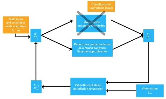
3.3. Data Assimilation Procedure

Given a trained patch-based NN representation as described in the previous section, we derive the associated Kalman-like filtering procedure. As summarized in Algorithm 1, at time step t, given the Gaussian approximation of the posterior likelihood $P\left(x_{t-1}\right|y_0,\dots ,y_{t-1})$ with mean $x_{t-1}^{+}$ and covariance ${\Sigma }_{t-1}^{+}$, we first compute the forecasted Gaussian approximation at time t with mean field $\mathcal{F}\left(x_{t-1}^{+}\right)$ and patch-based covariance ${\mathcal{F}}_{\Sigma }(x_{t-1}^{+},{\Sigma }_{t-1}^{+})$. The assimilation of the new observation $y_t$ is performed at a patch-level. For each patch ${\mathcal{P}}_s$, we update the patch-level mean $x_{{\mathcal{P}}_s,t}^{+}$ and covariance ${\Sigma }_{{\mathcal{P}}_s,t}^{+}$ using Kalman recursion (8) with observation $y_{{\mathcal{P}}_s,t}$. We then combine these patch-level updates to obtain global mean $x_t^{+}$ and covariance ${\Sigma }_t^{+}$. Whereas we compute global mean $x_t^{+}$ using trained reconstruction network ${\mathcal{F}}_r$, ${\Sigma }_t^{+}$ just comes to store the collection of patch-level covariances. This procedure is iterated up to the end of the observation sequence.

Algorithm 1 Patch-based NNKF reconstruction

1: procedure PB-NNKF($\mathcal{F}$,${\mathcal{F}}_{\Sigma }$,y,R)   2: for t in $[0,\dots ,T]$:   3:     $x_t^{-}\leftarrow \mathcal{F}\left(x_{t-1}^{+}\right)$   4:     $[{\Sigma }_{{\mathcal{P}}_0,t}^{-},\dots ,{\Sigma }_{{\mathcal{P}}_{N_p},t}^{-}]\leftarrow {\mathcal{F}}_{\Sigma }(x_{t-1}^{+},{\Sigma }_{t-1}^{+})$   5:     $[x_{{\mathcal{P}}_0,t}^{-},\dots ,x_{{\mathcal{P}}_{N_p},t}^{-}]\leftarrow ExtractPatches\left(x_t^{-}\right)$   6:     $[y_{{\mathcal{P}}_0,t},\dots ,y_{{\mathcal{P}}_{N_p},t}]\leftarrow ExtractPatches\left(y_t\right)$   7:     for s in $[1,\dots ,N_p]$:   8:        $K_{{\mathcal{P}}_s,t}={\Sigma }_{{\mathcal{P}}_s,t}^{-}{H}_{{\mathcal{P}}_s,t}^t{[H_{{\mathcal{P}}_s,t}{\Sigma }_{{\mathcal{P}}_s,t}^{-}{H}_{{\mathcal{P}}_s,t}^t+R_t]}^{-1}$   9:         $X_{{\mathcal{P}}_s,t}^{+}=x_{{\mathcal{P}}_s,t}^{-}+K_{{\mathcal{P}}_s,t}[y_{{\mathcal{P}}_s,t}-H_{{\mathcal{P}}_s,t}{x}_{{\mathcal{P}}_s,t}^{-}]$   10:         ${\Sigma }_{{\mathcal{P}}_s,t}^{+}={\Sigma }_{{\mathcal{P}}_s,t}^{-}-K_{{\mathcal{P}}_p,t}{H}_{{\mathcal{P}}_p,t}{\Sigma }_{{\mathcal{P}}_p,t}^{-}$   11:     $x_t^{+}\leftarrow Reconstruct([x_{{\mathcal{P}}_0,t}^{+},\dots ,x_{{\mathcal{P}}_{N_s},t}^{+}])$   12:     ${\Sigma }_t^{+}\leftarrow Reconstruct([{\Sigma }_{{\mathcal{P}}_0,t}^{+},\dots ,{\Sigma }_{{\mathcal{P}}_{N_s},t}^{+}])$

Compared with the patch-based analog data assimilation [22], it might be noted that we iterate patch-level assimilation steps and global reconstruction steps thanks to the NN-based propagation of the patch-based covariance structure. This procedure potentially allows information propagation from one patch to neighborhing ones after each assimilation step. By contrast, in the patch-based analog data assimilation, each patch is processed independently, such that no such information propagation can occur. This is regarded as a key feature to account for the propagation of geophysical structures (e.g., fronts, eddies, filaments,...).

We refer to the patch-based NNKF reconstruction model using the EOF block-diagonal parameterization of the covariance model ${\mathcal{F}}_{\Sigma }$, as model PB-NNKF-EOF. The model using the diagonal parameterization of the covariance model ${\mathcal{F}}_{\Sigma }$ in the patch space is referred to as PB-NNKF.

4. Data and Experimental Setting

As a case-study, we address the spatio-temporal interpolation of satellite-derived SST fields associated with infrared sensors, which may involve high missing data rates (typically from 50% to 90%). We consider the same region and dataset as in [22] to make easier benchmarking analysis.

4.1. Dataset Description

The SST time series used here is delivered by the UK Met Office [5] from January 2008 to December 2015. The spatial resolution of our SST field is $0.05$° and the temporal resolution $h=1$ day. The data from 2008 to 2014 were used as a training set. The 215 data were used as ground truth to provide a quantitative analysis, observations used in the assimilation experiments were simulated from this ground truth based on realistic SST clouds patterns provided by the METOP-AVHRR mask. This sensor is highly sensitive to the cloud cover and results in very high missing data rates.As case-study area, we select an area off South Africa (from $2.5$° E, $38.75$° S to $32.5$° E, $58.75$° S). This region involves is particularly relevant for the considered complex fine-scale SST dynamics (e.g., fronts, filaments). It makes it relevant for the considered quantitative and qualitative evaluation.

4.2. Experimental Setting

The proposed neural-network-based Kalman scheme involves the following parameter setting. The proposed patch-based and NN-based Kalman filter is applied to SST anomaly fields w.r.t. optimally-interpolated SST fields (see below for the parameterization of the optimal interpolation). These optimally-interpolated fields provide a relevant reconstruction of horizontal scales up to ≈100 km.

We exploit patch-level representations with non-overlapping $20\times 20$ patches. This patch size was particularly tuned for the resolution of fine scale structures for this particular dataset [22]. For each patch ${\mathcal{P}}_s$, we learn an EOF basis from the training data. We keep the first 50 EOF components, which amount on average to $95\%$ of the total variance. For the patch-level NN model ${\mathcal{F}}^{{\mathcal{P}}_s}$, we use a bilinear residual neural network architecture with 60 linear neurons, 100 bilinear neurons and 10 fully-connected layers with a Relu activation. Among other parametrizations [39], This architecture prove to outperform several othre data driven models in the forecasting of patch based SST dynamics. The reconstruction model ${\mathcal{F}}_r$ is a convolutional neural network with 3 convolutional layers. The first two layers comprise 64 filters of size $3\times 3$ with a Relu activation and the last layer is a linear convolutional layer with one filter. This parameters were tuned to give the best forecasting performances at a low computational cost.

Regarding the diagonal covariance model ${\mathcal{F}}_D^{{\mathcal{P}}_s}$, we consider an MLP with 4 layers, 3 hidden layers with 200 neurones and Relu activations and an output layer with a softplus activation. This parametrization was tunned to give the best trad-off between assimilation results and numerical complexity sins more complicated models lead to the same results illustrated in Section 5. With a view to evaluating the EOF-based covariance parameterization, we consider both PB-NNKF-EOF and PB-NNKF schemes.

We perform a quantitative analysis of the interpolation performance of the proposed scheme with respect to an optimal interpolation, and the EOF based interpolation method VE-DINEOF [11] which are two of the most popular techniques in spatio-temporal fields interpolation. Furthermore, in order to provide a comparison to an other data-driven data assimilation technique, we also tested the interpolation technique based on analog forecasting. Overall, the considered parameter setting is as follows:

• Optimal interpolation (OI): We use a Gaussian kernel with a spatial correlation length of 100 km and a temporal resolution length of 3 days. These parameters were empirically tuned for the considered dataset using a cross-validation experiment.
• Analog data assimilation (Local Analog Forecasting(LAF)-EnKF, Global Analog Forecasting(GAF)-EnKF): We apply both the global and local analog data assimilation schemes, referred to as GAF-EnKF, LAF-EnKF [19,22]. Similarly to the proposed scheme, we consider $20\times 20$ patches and 50-dimensional EOF decomposition with an overlapping of 10 pixels. We let the reader refer to [19,22] for a detailed description of this data-driven approach, which relies on nearest-neighbor regression techniques.
• EOF based reconstruction (PB-VE-DINEOF): We also compare our approach to the state-of-the-art interpolation scheme based on the projection of our observations with missing data on an EOF basis [11]. The SST field is here decomposed as described in the analog data assimilation application into a collection of $20\times 20$ patches with a 10 pixels overlapping. Each patch is then reconstructed using the VE-DINEOF method.

5. Results and Discussion

We report in this section the results of the considered numerical experiments. We first focus on patch-level performance as the patch-based representation is at the core of the proposed interpolation model. We then report interpolation performance for the whole case-study region.

5.1. Patch-Level Interpolation Performance

We first evaluate the patch-level interpolation performance of the proposed scheme for four patches corresponding to different dynamical modes as illustrated in Figure 2 located in the area (5° E to 75° E and latitude 25° S to 55° S). In

Table 1. Patch-level interpolation experiment: RMSE of the reconstructed anomaly fields for the LAF EnKF (local analog forecasting based ensemble Kalman filter), Bi-NN-EnKF (Bilinear residual neural net model (${\mathcal{F}}^{{\mathcal{P}}_s}$) used in an ensemble Kalman filter), Bi-NN-NNKF (Proposed NNKF based on a bilinear residual neural net dynamical mean model).

Assimilation Method	Considered Patch RMSE (°C)
	Patch 1	Patch 2	Patch 3	Patch 4
LAF EnKF	0.50	0.25	0.22	0.39
Bi-NN-EnKF	0.55	0.23	0.22	0.30
Bi-NN-NNKF-EOF	0.46	0.20	0.19	0.27

, we report the interpolation performance in terms of root mean square error (RMSE) for the proposed EOF NN-based scheme (NNKF-EOF) and include a comparison to the local analog data assimilation (LAF-EnKF). With a view to specifically analyzing the relevance of NN-based parametric covariance model, we also apply an ensemble Kalman filter with the trained dynamical model ${\mathcal{F}}^{{\mathcal{P}}_s}$. The reported results clearly illustrate the relevance of the proposed NN-based scheme for the assimilation of a single patch. The proposed NN-based scheme, which combines a NN-based formulation of the mean forecasting operator and of the associated covariance pattern, slightly outperforms the ensemble Kalman filters, while also significantly reducing the computational complexity induced by the generation of ensembles of size 500.

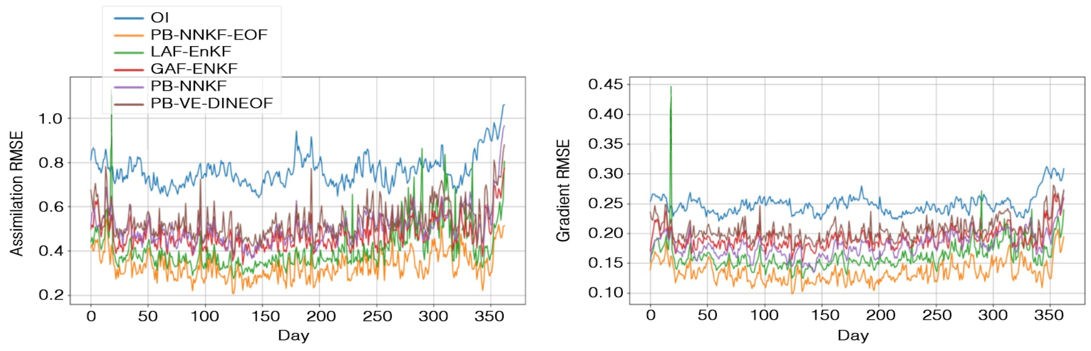
5.2. Global Forecasting and Interpolation Performances

Forecasting performances of the proposed data-driven dynamical priors: We further evaluate the performance of the proposed schemes over the considered case-study region.

Table 2. Forecasting experiment for several prediction time steps.

Model	Forecasting RMSE (°C)
	t+h	t+4h	t+8h
PB-NN	0.48	0.60	0.63
LAF	0.50	0.68	0.76
GAF	0.61	0.74	0.76

reports the RMSE of the proposed NN-based representation compared with local and global forecasting operator [19]. The proposed patch-level NN-based model outperforms the benchmarked approaches by about 5–15% in terms of forecasting RMSE. This is due to the structure of the proposed model that involves a postprocessing operator learnt from data that combines the predicted patches in order to minimize the global forecasting error. The analog forecasting models in the other hand, even through the use of more patches with overlapping, process the output patches through EOF projections to get ride of the variability due to the patches interaction. However, This smoothing results in losing some high resolution information which results in diminishing the forecasting results with respect to our proposed model.

Interpolation performances of the proposed model with respect to OI and DINEOF: We report the mean interpolation performance in

Table 3. SST interpolation experiment: Reconstruction correlation coefficient and RMSE over the SST time series and their gradient.

Model	Entire Map				Missing Data Areas
	RMSE		Correlation		RMSE		Correlation
	$\mathbf{SST}(°\mathbf{C})$	$\nabla \mathbf{SST}(°\mathbf{C}/°)$	$\mathbf{SST}$	$\nabla \mathbf{SST}$	$\mathbf{SST}(°\mathbf{C})$	$\nabla \mathbf{SST}(°\mathbf{C}/°)$	$\mathbf{SST}$	$\nabla \mathbf{SST}$
PB-NNKF-EOF	0.33	0.13	99.87%	89.30%	0.35	0.10	99.85%	93.49%
PB-NNKF	0.51	0.18	99.75%	81.24%	0.51	0.18	99.71%	81.50%
LAF-EnKF	0.43	0.16	99.79%	84.41%	0.42	0.15	99.77%	86.73%
GAF-EnKF	0.48	0.19	99.74%	79.12%	0.48	0.18	99.72%	80.74%
PB-VE-DINEOF	0.54	0.20	99.68%	75.30%	0.54	0.21	99.66%	74.71%
OI	0.76	0.25	99.37%	60.31%	0.75	0.27	99.37%	55.73%

and the interpolation error time series in Figure 3. The proposed NN-based scheme (PB-NNKF-EOF) leads to very significant improvements with respect to the optimal interpolation and PB-VE-DINEOF schemes in terms of RMSE and correlation coefficients for both the SST and its gradient with a relative improvement of the RMSE above 50% for missing data areas for the SST and its gradient (resp. 40%). This important gain clearly emphasizes retrivement of fine scale structures unresolved using OI and DINEOF techniques. From a methodological point of view, this gain was clearly expected. OI and DINEOF schemes rely purely on data to interpolate the SST field. Therefore when provided with observations with a high missing data rate, these techniques are only able to retrive horizontal scales up to ≈100 km. In the opposite, our proposed framework combines both the observations and the data driven model outputs to reconstruct our SST field which results in better representation of fine scale structures.

Interpolation performances of the proposed model with respect to GAN-EnKF, LAN-EnKF: A clear gain is also exhibited w.r.t. analog data assimilation schemes with a relative gain greater than 20% in terms of RMSE for both the SST and its gradient. The same conclusion holds in terms of correlation coefficients close to 90% or above for all parameters for PB-NNKF-EOF scheme, all the other ones depicting correlation coefficients below 85% for SST gradient fields. These results reflect the forecasting performances illustrated in Table 2 and the patch based interpolation performances in Table 1. Indeed, the PB-NNKF-EOF scheme outperforms both the analog forecasting operators in terms of one step ahead predictions which suggest better assimilation in a global scale especially for missing data areas. Although the considered NN-based representation exploits non-overlapping patches, we still come up with significant improvements w.r.t AnDA schemes which involve a 50% overlapping rate between patches. This clearly illustrates the relevance of NN-based representation, which fully embeds the direct and inverse mappings between the SST field and its patch-level representation. Iterating patch-level assimilation steps and global reconstruction steps as illustrated by the Algorithme 1 allows information propagation of assimilated patches in a global scale which helps outperforming AnDA schemes. Interestingly, Table 3 also reveals the importance of the EOF-based parameterization of the NN-based covariance model (19) in the improvement of interpolation results.

Qualitative analysis of the proposed schemes: We further illustrate these conclusions through interpolation examples in Figure 4. The visual analysis of the reconstructed SST gradient fields emphasize the relevance of PB-NNKF-EOF scheme to reconstruct fine-scale details. While OI and PB-VE-DINEOF schemes tend to smooth out fine-scale patterns, the analog data assimilation may not account appropriately for patch boundaries. This typically requires an empirical post-processing step [22]. By contrast, the PB-NNKF-EOF scheme fully embeds this post-processing step through reconstruction network ${\mathcal{F}}_r$ and learns its parameterization from data, which is shown here to greatly improve patch-based interpolation performance. The analysis of the spectral signatures in Figure 5 leads to similar conclusions with the PB-NNKF-EOF scheme being the only one to recover significant energy level up to 50 km.

6. Conclusions

In this work, we addressed neural-network-based models for the spatio-temporal interpolation of satellite-derived SST fields. We introduced a novel probabilistic NN-based representation of geophysical dynamics. This representation, which relies on a patch-level and EOF-based decomposition, allows us to propagate in time a mean component and the covariance of the SST field. It makes direct the derivation of an associated Kalman filter for the spatio-temporal interpolation of SST dynamics. The relevance of the proposed framework is demonstrated in our numerical experiments with respect to the state-of-the-art approaches. Our method clearly outperforms the optimal interpolation and DINEOF based schemes which fail retrieving fine scale structures due to the high missing data rate in our observations. Comparing our data-driven data assimilation scheme to the analog data assimilation framework reveals the importance of investigating such filtering representations. From our numerical experiments, an important gain is stressed with respect to analog forecasting based schemes which is principally due to the formulation of our stochastic dynamical model. The patch based identification procedure allows to significantly reduce the identification complexity while still giving good priors. The recollection of the patches to form the global output allows getting ride of fine tuning post-processing step that can decrease the results as illustrated in our experiments. Finally the stochastic formulation of our dynamical model allows the propagation of a parametric PDF of our transition function in a Kalman like assimilation scheme. This stochastic formulation is completely learnt from data and allows getting ride of the ensemble formulation that may cause limitations in terms of numerical complexity.

We believe that this study opens a new research avenue for the design of stochastic dynamical representations for spatio-temporal fields. The application of the proposed framework to other sea surface geophysical tracers, including multi-source and multi-modal interpolation issues is considered as our first priority. SLA (Sea Level Anomaly) fields could provide an interesting case-study as the associated space-time sampling is particularly scarce and multi-source strategies are of key interest [40]. Improving the formulation and training of the covariance model is also an important issue. Learning our covariance model based on one step ahead ensemble forecasting is most likely to fail in sequential assimilation frameworks when provided with observations with highly irregular temporal sampling. Optimizing our covariance model based on the spatio-temporal sampling of our observations seems to be an interesting path to investigate as one of our further works.

The use of the RMSE for training our data-driven models and as a diagnosis tool raises the question of the relevance of the proposed criterion. Although from the qualitative analysis based on the visual analysis of our reconstructed fields proved the relevance of the proposed technique. The development of more rigorous diagnosis and training criterions based on structures matching is an appalling research avenue. Exploiting stability analysis tools such as Lyapunov exponents is an interesting approach that may increase the modeling capabilities of our data-driven framework.

Finally, the interpretation of the parametrization of the reconstruction network is an open issue. In our work, our reconstruction network was tuned to give the best forecasting performances with a low computational complexity. However, defining a relationship between the reconstruction network parameters (e.g., number of filters, kernel size, activation function) and the physical system (e.g., fine scale structures identification, patch boundaries) is an open research topic that might be answered in the next years due to the advances of deep learning interpretability.

References

1. Hardman-Mountford, N.J.; Richardson, A.J.; Boyer, D.C.; Kreiner, A.; Boyer, H.J. Relating sardine recruitment in the Northern Benguela to satellite-derived sea surface height using a neural network pattern recognition approach. Prog. Oceanogr. 2003, 59, 241–255. [Google Scholar] [CrossRef]
2. Le Traon, P.Y. Satellites and operational oceanography. In Operational Oceanography in the 21st Century; Springer: Berlin/Heidelberg, Germany, 2011; pp. 29–54. [Google Scholar]
3. Von Schuckmann, K.; Le Traon, P.Y.; Alvarez-Fanjul, E.; Axell, L.; Balmaseda, M.; Breivik, L.A.; Brewin, R.J.; Bricaud, C.; Drevillon, M.; Drillet, Y. The copernicus marine environment monitoring service ocean state report. J. Oper. Oceanogr. 2016, 9, s235–s320. [Google Scholar] [CrossRef]
4. Escudier, R.; Bouffard, J.; Pascual, A.; Poulain, P.M.; Pujol, M.I. Improvement of coastal and mesoscale observation from space: Application to the northwestern Mediterranean Sea. Geophys. Res. Lett. 2013, 40, 2148–2153. [Google Scholar] [CrossRef] [Green Version]
5. Donlon, C.J.; Martin, M.; Stark, J.; Roberts-Jones, J.; Fiedler, E.; Wimmer, W. The Operational Sea Surface Temperature and Sea Ice Analysis (OSTIA) system. Remote Sens. Environ. 2012, 116, 140–158. [Google Scholar] [CrossRef]
6. Le Traon, P.Y.; Nadal, F.; Ducet, N. An improved mapping method of multisatellite altimeter data. J. Atmos. Ocean. Technol. 1998, 15, 522–534. [Google Scholar] [CrossRef]
7. Droghei, R.; Buongiorno Nardelli, B.; Santoleri, R. A New Global Sea Surface Salinity and Density Dataset From Multivariate Observations (1993–2016). Front. Mar. Sci. 2018, 5, 84. [Google Scholar] [CrossRef]
8. Nardelli, B.B.; Pisano, A.; Tronconi, C.; Santoleri, R. Evaluation of different covariance models for the operational interpolation of high resolution satellite Sea Surface Temperature data over the Mediterranean Sea. Remote Sens. Environ. 2015, 164, 334–343. [Google Scholar] [CrossRef]
9. Ducet, N.; Le Traon, P.Y.; Reverdin, G. Global high-resolution mapping of ocean circulation from TOPEX/Poseidon and ERS-1 and-2. J. Geophys. Res. Oceans 2000, 105, 19477–19498. [Google Scholar] [CrossRef]
10. Gomis, D.; Ruiz, S.; Pedder, M.A. Diagnostic analysis of the 3D ageostrophic circulation from a multivariate spatial interpolation of CTD and ADCP data. Deep Sea Res. Part I Oceanogr. Res. Pap. 2001, 48, 269–295. [Google Scholar] [CrossRef] [Green Version]
11. Ping, B.; Su, F.; Meng, Y. An Improved DINEOF Algorithm for Filling Missing Values in Spatio-Temporal Sea Surface Temperature Data. PLoS ONE 2016, 11, e0155928. [Google Scholar] [CrossRef] [PubMed]
12. Olmedo, E.; Taupier-Letage, I.; Turiel, A.; Alvera-Azcárate, A. Improving SMOS Sea Surface Salinity in the Western Mediterranean Sea through Multivariate and Multifractal Analysis. Remote Sens. 2018, 10, 485. [Google Scholar] [CrossRef]
13. Alvera-Azcárate, A.; Barth, A.; Parard, G.; Beckers, J.M. Analysis of SMOS sea surface salinity data using DINEOF. Remote Sens. Environ. 2016, 180, 137–145. [Google Scholar] [CrossRef]
14. Beckers, J.M.; Rixen, M. EOF Calculations and Data Filling from Incomplete Oceanographic Datasets. J. Atmos. Ocean. Technol. 2003, 20, 1839–1856. [Google Scholar] [CrossRef]
15. Bertino, L.; Evensen, G.; Wackernagel, H. Sequential Data Assimilation Techniques in Oceanography. Int. Stat. Rev. 2007, 71, 223–241. [Google Scholar] [CrossRef] [Green Version]
16. Lorenc, A.C.; Ballard, S.P.; Bell, R.S.; Ingleby, N.B.; Andrews, P.L.F.; Barker, D.M.; Bray, J.R.; Clayton, A.M.; Dalby, T.; Li, D.; et al. The Met. Office global three-dimensional variational data assimilation scheme. Q. J. R. Meteorol. Soc. 2000, 126, 2991–3012. [Google Scholar] [CrossRef]
17. Yablonsky, R.M.; Ginis, I. Limitation of One-Dimensional Ocean Models for Coupled Hurricane–Ocean Model Forecasts. Mon. Weather Rev. 2009, 137, 4410–4419. [Google Scholar] [CrossRef]
18. van Leeuwen, P.J. Nonlinear data assimilation in geosciences: An extremely efficient particle filter. Q. J. R. Meteorol. Soc. 2010, 136, 1991–1999. [Google Scholar] [CrossRef]
19. Lguensat, R.; Tandeo, P.; Ailliot, P.; Pulido, M.; Fablet, R. The Analog Data Assimilation. Mon. Weather Rev. 2017, 145, 4093–4107. [Google Scholar] [CrossRef]
20. Tandeo, P.; Ailliot, P.; Chapron, B.; Lguensat, R.; Fablet, R. The analog data assimilation: Application to 20 years of altimetric data. In Proceedings of the 5th International Workshop on Climate Informatics, Boulder, CO, USA, 24–25 September 2015; pp. 1–2. [Google Scholar] [CrossRef]
21. Lguensat, R.; Huynh Viet, P.; Sun, M.; Chen, G.; Fenglin, T.; Chapron, B.; Fablet, R. Data-Driven Interpolation of Sea Level Anomalies Using Analog Data Assimilation. 2017. Available online: https://hal.archives-ouvertes.fr/hal-01609851 (accessed on 22 November 2018).
22. Fablet, R.; Viet, P.H.; Lguensat, R. Data-Driven Models for the Spatio-Temporal Interpolation of Satellite-Derived SST Fields. IEEE Trans. Comput. Imaging 2017, 3, 647–657. [Google Scholar] [CrossRef]
23. Pannekoucke, O.; Emili, E.; Thual, O. Modelling of local length-scale dynamics and isotropizing deformations. Q. J. R. Meteorol. Soc. 2013, 140, 1387–1398. [Google Scholar] [CrossRef]
24. Pannekoucke, O.; Ricci, S.; Barthelemy, S.; Ménard, R.; Thual, O. Parametric Kalman filter for chemical transport models. Tellus A Dyn. Meteorol. Oceanogr. 2016, 68, 31547. [Google Scholar] [CrossRef]
25. Rezende, D.J.; Mohamed, S.; Wierstra, D. Stochastic Backpropagation and Approximate Inference in Deep Generative Models. arXiv, 2014; arXiv:1401.4082. [Google Scholar]
26. Matthews, A.G.d.G.; Rowland, M.; Hron, J.; Turner, R.E.; Ghahramani, Z. Gaussian Process Behaviour in Wide Deep Neural Networks. arXiv, 2018; arXiv:1804.11271. [Google Scholar]
27. Fablet, R.; Ouala, S.; Herzet, C. Bilinear residual Neural Network for the identification and forecasting of dynamical systems. arXiv, 2017; arXiv:1712.07003. [Google Scholar]
28. Egmont-Petersen, M.; de Ridder, D.; Handels, H. Image processing with neural networks—A review. Pattern Recognit. 2002, 35, 2279–2301. [Google Scholar] [CrossRef]
29. Braakmann-Folgmann, A.; Roscher, R.; Wenzel, S.; Uebbing, B.; Kusche, J. Sea Level Anomaly Prediction using Recurrent Neural Networks. arXiv, 2017; arXiv:1710.07099. [Google Scholar]
30. Taormina, R.; Chau, K.W.; Sivakumar, B. Neural network river forecasting through baseflow separation and binary-coded swarm optimization. J. Hydrol. 2015, 529, 1788–1797. [Google Scholar] [CrossRef]
31. Evensen, G. Data Assimilation; Springer: Berlin/Heidelberg, Germany, 2009. [Google Scholar] [CrossRef]
32. Anderson, J.L.; Anderson, S.L. A Monte Carlo Implementation of the Nonlinear Filtering Problem to Produce Ensemble Assimilations and Forecasts. Mon. Weather Rev. 1999, 127, 2741–2758. [Google Scholar] [CrossRef]
33. Houtekamer, P.L.; Mitchell, H.L. Data Assimilation Using an Ensemble Kalman Filter Technique. Mon. Weather Rev. 1998, 126, 796–811. [Google Scholar] [CrossRef] [Green Version]
34. Gaspari, G.; Cohn, S.E. Construction of correlation functions in two and three dimensions. Q. J. R. Meteorol. Soc. 1999, 125, 723–757. [Google Scholar] [CrossRef] [Green Version]
35. Houtekamer, P.L.; Mitchell, H.L. A Sequential Ensemble Kalman Filter for Atmospheric Data Assimilation. Mon. Weather Rev. 2001, 129, 123–137. [Google Scholar] [CrossRef]
36. Bocquet, M. Localization and the iterative ensemble Kalman smoother. Q. J. R. Meteorol. Soc. 2016, 142, 1075–1089. [Google Scholar] [CrossRef]
37. Cohn, S.E. Dynamics of Short-Term Univariate Forecast Error Covariances. Mon. Weather Rev. 1993, 121, 3123–3149. [Google Scholar] [CrossRef] [Green Version]
38. LeCun, Y.; Haffner, P.; Bottou, L.; Bengio, Y. Object Recognition with Gradient-Based Learning. In Shape, Contour and Grouping in Computer Vision; Forsyth, D.A., Mundy, J.L., di Gesú, V., Cipolla, R., Eds.; Lecture Notes in Computer Science; Springer: Berlin/Heidelberg, Germany, 1999; pp. 319–345. [Google Scholar] [CrossRef]
39. Ouala, S.; Herzet, C.; Fablet, R. Sea surface temperature prediction and reconstruction using patch-level neural network representations. arXiv, 2018; arXiv:1806.00144. [Google Scholar]
40. Fablet, R.; Verron, J.; Mourre, B.; Chapron, B.; Pascual, A. Improving Mesoscale Altimetric Data From a Multitracer Convolutional Processing of Standard Satellite-Derived Products. IEEE Trans. Geosci. Remote Sens. 2018, 56, 2518–2525. [Google Scholar] [CrossRef] [Green Version]
Figure 1. Proposed neural-network-based representation of a spatio-temporal dynamical system. The input X t is first decomposed into P × P patches, each patch is then propagated using its associate local stochastic dynamical models ( F P s , F Σ P s ) . The mean componont of the output X t + 1 is reconstructed by injecting the forecasted patches into the reconstruction model F r . The block diagonal covariance matrix is formed by the collection of the patch-level covariances.
Remotesensing 10 01864 g001
Figure 2. Selected patches on the high resolution component of the SST data. (The SST map corresponds to 19 July 2015).
Remotesensing 10 01864 g002
Figure 3. Reconstruction and gradient RMSE times series for the selected models.
Remotesensing 10 01864 g003
Figure 4. Interpolation of the SST field on 19 July 2015: first row, the reference SST, its gradient and the observation with missing data (here, 82% of missing data); second row, interpolation results using respectively OI, PB-VE-DINEOF, GAF-EnKF, LAF-EnKF, PB-NN-NNKF, PB-NN-NNKF-EOF; third row, gradient of the reconstructed fields.
Remotesensing 10 01864 g004
Figure 5. Radially averaged power spectral density of the interpolated SST fields with respect to the reference SST.
Remotesensing 10 01864 g005