Article

Landscape-Scale Aboveground Biomass Estimation in Buffer Zone Community Forests of Central Nepal: Coupling In Situ Measurements with Landsat 8 Satellite Data

1
Graduate School of Agricultural and Life Sciences, University of Tokyo, 1-1-1 Yayoi, Bunkyo-Ku, Tokyo 113-8567, Japan
2
Institute for Water Studies, Department of Earth Sciences, University of the Western Cape, Private Bag X17, Bellville 7535, South Africa
*
Author to whom correspondence should be addressed.
Remote Sens. 2018, 10(11), 1848; https://doi.org/10.3390/rs10111848
Submission received: 29 October 2018 / Revised: 17 November 2018 / Accepted: 19 November 2018 / Published: 21 November 2018
(This article belongs to the Section Remote Sensing in Agriculture and Vegetation)

Abstract

:
Knowledge of forest productivity status is an important indicator of the amount of biomass accumulated and the role of terrestrial ecosystems in the carbon cycle. However, accurate and up-to-date information on forest biomass and forest succession remain rudimentary within natural forests. This study sought to understand and establish the potential of a new-generation sensor in estimating aboveground biomass (AGB) stored in the natural forest, also known as ‘community forest’ or buffer zone community forest (BZCF), in the Parsa National Park, Nepal. The utility of the 30-m resolution Landsat 8 Operational Land Imager (OLI) and in situ data was tested using two statistical approaches, namely multiple linear regression (MLR) and random forest (RF). The analysis was done based on four computational procedures. These included spectral bands, vegetation indices and pooled dataset (spectral bands + vegetation indices), and model selected important variables. AGB estimation based on pooled data showed that the RF algorithm produced better results when compared to the use of the MLR model. For instance, the RF model estimated AGB with an R2 value of 0.87 and a root mean square error of 20.50 t ha−1, as well as an R2 value of 0.95 and a RMSE of 13.3 t ha−1 when using selected important variables. Comparatively, the MLR using pooled data produced an R2 value of 0.56 and RMSE value of 37.01 t ha−1. The RF model selected Optimized Soil Adjusted Vegetation index (OSAVI), Simple ratio (SR), Modified simple ratio (MSR), and Normalized difference Vegetation index (NDVI) as the most important variables for estimating AGB, whereas MLR selected band 5 and SR. These findings demonstrate the relevance of the relatively new Landsat 8 sensor in the estimation of AGB in community buffer zones.

Graphical Abstract

1. Introduction

The concept of buffer zones was introduced to concurrently alleviate human development pressure in conservation areas and address the socioeconomic requirements of affected populations without jeopardizing natural ecosystems [1]. The initiative was also introduced to help resolve potential conflicts over the usage of forest and forest products [2]. Irrespective of these efforts, challenges still remain as the use of forest resources has drastically increased over the years, rendering the whole process unsustainable [2]. There is, therefore, an urgent need to routinely and accurately assess the impacts of human activities on the productivity of these protected ecosystems. This information is critical in determining and providing baseline insights into the productivity of these forests and to develop well-informed management practices.
The lack of spatially explicit methods or frameworks for assessing productivity in community buffer zones has hampered knowledge on the productivity of these ecosystems and their role in the carbon cycle. Available information has been gathered through the use of traditional monitoring techniques, which include routine surveys and point-based AGB estimates. These methods, although accurate, have not produced the intended outcomes as they are spatially restricted and labor-intensive, especially when it comes to regional-scale monitoring [3]. For instance, traditional field-based biomass estimation methods are no doubt more accurate [4], but the major challenge with them is that they are time-consuming, laborious, and difficult to implement in inaccessible areas, besides being very destructive. Remote sensing is hypothetically a cost-effective technique, which provides the most accessible alternative as it offers spatially explicit data and enables repeated monitoring, even in remote locations [5]. For instance, Clark et al. [6], Chen et al. [7], Dube et al. [8], Mutanga et al. [9], and Rana et al. [10] satisfactorily predicted AGB based on hyperspectral, LiDAR (Light detection and ranging), and medium-resolution sensors together with field data. Of all the sensors, hyperspectral sensors have been found to provide some of the best datasets in biomass estimation.
However, hyperspectral datasets are often associated with limited spatial coverage, due to their acquisition cost, limited availability, and huge data volumes, as well as large data preprocessing costs [11]. The limitations of using hyperspectral remote sensing technologies have also been cited by Mathieu et al. [12]. Thus, the free Landsat program remains one of the most important primary data sources, due to the presence of archival data (dating back to 1972) and the rich spectral information, with relatively moderate spatial resolution (30 m) for forest biophysical investigation. Additionally, it is freely accessible data, with a global footprint (185-km swath width) and good monitoring in developing countries, where the cost of hyperspectral data remains a problem. The latest research portrays Landsat 8 products as being more reliable in AGB estimation and monitoring [11]. For example, Karlson et al. [13] successfully evaluated the utility of Landsat 8 data for mapping tree canopy cover and aboveground biomass in the woodland landscape in Burkina Faso. Similarly, findings by Dube and Mutanga [11] concluded that Landsat 8 OLI bands can improve AGB accuracies when compared to its predecessors.
Despite these rapid advancements in remote sensing and their strong potential for use in investigating forest biophysical attributes, only a few AGB estimation studies have been conducted in tropical and subtropical forests and, ultimately, carbon estimates in Nepal. For example, Karna et al. [14] used WorldView-2 satellite images with small-footprint airborne LiDAR data to estimate tree carbon stocks in a tropical forest in Nepal. Similarly, Baral [3] integrated GeoEye and WorldView-2 to estimate carbon stocks in subtropical forests in central Nepal with high accuracy. Most of the studies in Nepal focused on tropical and subtropical forests, mainly because of the diversity of flora and fauna in these ecosystems [15], but with few detailed ground-based quantifications of biomass [3]. Likewise, Murthy et al. [16] used LiDAR and field data to create a national forest inventory (for the period 2010–2014) for Nepal. These studies, however, created good baseline data that could be used for both future applications and REDD+ (Reducing Emissions from Deforestation and Forest Degradation, plus other conservation activities) monitoring, reporting, and verification. Some attempts have also been made to explore the potential of medium-resolution imagery for forest interpretation, as well as for mapping forest cover and volume. For instance, Muinonen et al. [17] used Landsat TM (Thematic Mapper) and MODIS (Moderate Resolution Imaging Spectroradiometer) data to map forest cover and total stand volume in western and eastern Nepal. Nevertheless, prior Landsat products have since developed scan line problems, complicating forestry and biomass estimation endeavors, as well as the REDD+ annual reporting at the national level [18]. Although not yet sufficiently tested, the contemporary Landsat 8 thus remains the most accessible remote sensing product readily available for biomass and forest monitoring at a national or regional scale.
The existing Landsat 8 OLI sensor has several improvements over its predecessors, the TM and ETM+ (Enhanced Thematic Mapper Plus). These enhancements include an increased number of spectral bands, improved radiometric resolution from 8 bits to 12 bits [19], and a refined spectral range for certain bands, which is likely to improve the vegetation spectral response across the near-infrared and panchromatic bands, as well as an improved signal-to-noise ratio using two push-broom sensors [20] that are almost twice as good as those in the Landsat 7 ETM+. The enhanced radiometric resolution improves the spectral record precision and avoids the spectral saturation seen in previous studies using Landsat data [21,11]. One of the major forest AGB estimation challenges in Nepal is the lack of baseline data on forest resources from the local to the regional level. This remains one of the prominent issues where the capacity of the forest staff in the field to carry out inventory is very limited. The reason may be due to the absence of technical support and overdependence mostly on traditional methods of field data collection. The objective of the study was, therefore, to test the utility of relatively new Landsat 8 OLI data in estimating above-ground biomass in natural forest in the Parsa National Park, Nepal, based on two robust statistical approaches: multiple linear regression (MLR) and random forest (RF). This research constitutes a concerted effort to fill the gaps in AGB data in Nepalese forestry.

2. Materials and Methods
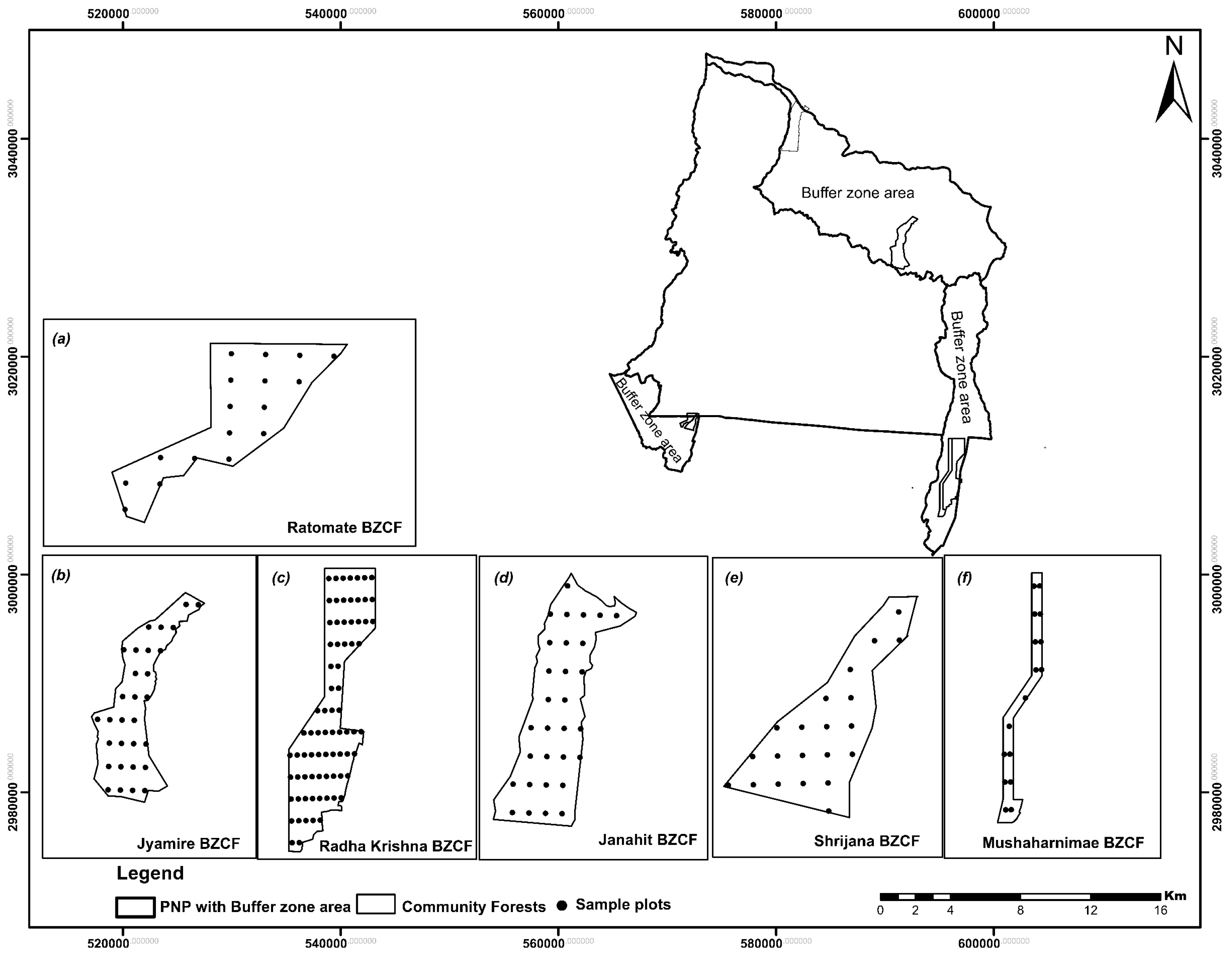
2.1. Study Area

The study area, the Parsa National Park (PNP), is located within the central lowlands of Nepal between latitude 27°28′0′′N and longitude 84°20′0′′E. Six buffer zone community forests were selected for the establishment of sample plots (Figure 1). All the forests are managed by Buffer Zone community forest user groups. The vegetation is tropical to subtropical forest (mainly deciduous), and the selected forests were dominated by sal (Shorea robusta) followed by red berry (Mallotus philippensis), duabanga (Duabanga grandiflora), axlewood (Anogeissus latifolia), and jamun (Syzygium cumini). The topography is generally flat, with minor variations in elevation (100 to 807 m above sea level), and the soil is primarily alluvial in the lower belt, but gravel and conglomerates are found with increasing elevation. As the altitude increases in the north along the Churia Hills, Shorea robusta is gradually replaced by Pinus roxburghii. The area is characterized by subtropical climatic conditions, with mean annual precipitation of 1908 mm and a mean annual temperature of 24.5 °C recorded during 1981–2010. Winters are cold, with morning fog lasting until noon and sometimes longer.

2.2. Field Measurements

Field surveys were conducted from 24 February to 12 March 2016. A circular plot size of 500 m2 was used during data collection. In total, 173 plots were gathered, of which 113 plots’ data were collected during the field survey. The remaining 60 plots’ data were provided by the Parsa National Park authorities. These plots were generated in ArcGIS version 10.3 (ESRI, Redlands, CA, USA) using a systematic random sampling technique. The reason for adopting this methodology was to ensure uniformity in the sampling, and it is in line with the PNP sampling procedure. The PNP is largely characterized by almost uniform forest types and species distribution; thus, we chose to vary the species samples between plots considering the size of the forest in order to minimize the required time and labor. The forest area varied between 66 and 650 ha. Within plots, structural variables, namely diameter at breast height (DBH) ≥5 cm (1.3 m above the ground) and tree height (H), were measured using a DBH measuring tape (Yamayo measuring tools Co. Ltd., Tokyo, Japan) and a Hypsometer vertex laser (Laser Technology, Inc., Colorado, USA) instrument, respectively.

2.3. Field-Based AGB

Tree-level AGB was derived using the species-specific allometry developed by Chave et al. [22]. The models were developed specifically for tree species occurring within a specified climate zone; thus, forest types and climatic characteristics in the PNP were similar to those used in developing a tree-specific model. The guidelines published by ANSAB (Asia Network for Sustainable Agriculture and Bioresources) [23] suggest that the model (Equation 1) is appropriate for moist forest stands, with annual precipitation of 1500 to 4000 mm. These were similar to the climatic conditions prevailing in the study area. This method is also recommended by the Ministry of Forest and Soil Conservation, Nepal. Specific gravity values suggested by Chaturvedi and Khanna [24] were used for individual tree species; particularly, for those species without such values, a general tropical species value (ρ = 0.674) was used. Individual biomass for all trees within the plot was calculated using Equation 1 and then aggregated to obtain plot-level AGB. The biomass resulting from the model was standardized by converting the value into tonnes per hectare (t ha−1).
  AGB = 0.0509 × ρ D 2 H  
where AGB is aboveground biomass (kg); ρ is specific gravity (g cm−3); D is diameter at breast height (cm), H is tree height (m), and the constant 0.0509 was obtained from the work by Chave et al. [22].

2.4. Image Acquisition and Data Processing

Landsat 8 OLI imagery was chosen as the primary spatial data source to estimate AGB in the PNP community forest. This data was chosen because of its convenient procurability and the suitable spectral and spatial resolutions. The image was acquired on a sunny, clear day with 0.24% cloud cover. The satellite image was obtained from the freely accessible United States Geological Survey EROS (Earth Resources Observation and Science) Center Archive. The Landsat 8 OLI sensor was launched on 11 February 2013 and has a 16-day temporal resolution. Onboard, there are two push-broom instruments: (i) the OLI, consisting of nine spectral bands, and (ii) the Thermal Infrared Sensor, which encompasses thermal bands 10 and 11 at a 100-m spatial resolution. These improvements may enable greater accuracy in mapping the AGB of BZCFs. The study area was covered by only one Landsat scene (path/row: 141/41). The applied Landsat 8 OLI imagery, with the L1T (systematic precision and terrain-corrected) product, was acquired on 7 October 2015. The downloaded image was georeferenced using the WGS84, UTM Zone 45N coordinate system.
The Landsat image scene was obtained in digital numbers, and was therefore converted to reflectance values. First, the Landsat OLI image spectral bands were converted to top-of-atmosphere spectral radiances and then to sensor reflectance in ENVI classic version 5.3 (Harris Corporation, Blvd. Melbourne, USA). We performed atmospheric correction using a FLAASH (Fast Line-of-Sight Atmospheric Analysis of Spectral Hypercube) radiative transfer model [25].

2.5. Deriving Spectral Data and Vegetation Indices

Field survey points were overlaid on the corrected image to generate regions of interest, using the central (x, y) coordinates obtained by using a Garmin 62s global positioning system for all 173 plots. The same image pixel size (30 × 30) was considered to extract vegetation spectral values for each band (bands 1 to 7). The spectra were extracted using the ENVI software, and these were then averaged for each plot. The extracted values were then used to calculate vegetation indices, which were further used together with spectral bands to estimate AGB. Detailed information on the spectral bands and vegetation indices (VIs) considered in this study is summarized in Table 1. The applied vegetation indices were chosen based on recommendations from previous forest biomass research conducted across the world [26]. In addition, variable selection was implemented to select key AGB variables from all the variables used (spectral bands and VIs). The important VIs selected for the final RF model are given in Table 2.

2.6. Modeling Methods and Model Precision Assessment

To establish a relationship between the field-measured biomass and remote-sensing variables, the field-measured AGB was considered as a dependent variable, whereas spectrally derived variables were treated as the response variables. Two modeling approaches were used: MLR and RF. Ten-fold cross-validation was used in both models. This was informed by the limited number of sample plots used in AGB estimation. The regression was performed in R software (R Development Core Team) [35], using a “boot” package [36] for linear modeling, a “faraway” package [37] for the variance inflation factor, and “caret” [38] for cross-validation, and the “randomForests” package [39] for random forest modeling.

2.6.1. Multiple Linear Regression

Multiple linear regression is a parametric algorithm that has been commonly used in biomass estimation [40]. Because the MLR has the ability to deal with dependencies on or correlations with the predictors very well, we therefore chose to explore its strength for complex forest biomass estimation. One of the advantages of this model is that it can select the suitable variables for the regression model when many explanatory variables are employed. The basic idea of this algorithm is that it can introduce all the explanatory variables into the regression in backward mode, that is, when multiple variables are being regressed. In addition, the method simultaneously removes unimportant variables in explaining the variation in the dependent variable. The model with the lower AIC (Akaike information criterion) was considered. Finally, in the regression method, independent variables were also analyzed for multicollinearity using the variance inflation factor (VIF). To determine multicollinearity problems, a VIF value less than 10 was considered [41]. Variables with the largest VIF were then removed; thus, the final model was run using noncollinear variables. Our main assumption for choosing the MLR was that the dependent variable consisted of numerical data and was normally distributed. To check the normality of the data, we applied the Shapiro–Wilk test [42] and the Anderson–Darling test [43] (W = 0.99, p = 0.54; A = 0.187, P = 0.90, respectively). Lastly, the error term was homoscedastic (Breuch–Pagan test and White test). For AGB estimation, statistical analysis was implemented based on three analysis sets: (i) spectral bands only, (ii) vegetation indices only, and (iii) pooled data (spectral bands and vegetation indices).

2.6.2. Random Forest

The RF model is a type of ensemble machine-learning algorithm called bootstrap aggregation or bagging, where a number of trees (ntree) is constructed on the basis of a random subset of samples drawn from the training data [26]. The RF regression algorithm utilizes bootstrap samples from the training data without pruning to grow a large number of decision trees [44,45,46]. These trees assign each predictor variable (ISI or VIs) to a response variable (in this case, AGB) using the average estimate that the value receives from the collection of all trees [46]. Furthermore, at each node of the decision tree, selection of the features for modeling is also stochastic, making the approach immune to the problem of overfitting [47]. Therefore, there are two important parameters, namely mtry, which is denoted as the number of variables available for splitting at each node of the tree, and ntree, termed as the “tuning parameters”. The RF algorithm is easy to implement, as only two parameters (mtry and ntree) need to be optimized to achieve the desirable prediction (selecting the least RMSE) [47,48,49]. The tuning of the parameters depends on the user, and the tuning can vary from using a too-high value to a too-low value [50]. The default value for the ntree parameter is 500 trees, and that for mtry is 1/3 of the total number of variables used in the model. Also, another important parameter is nodesize, as mentioned by Scornet et al. [51], which was set to the default value of 1, as suggested in the literature.

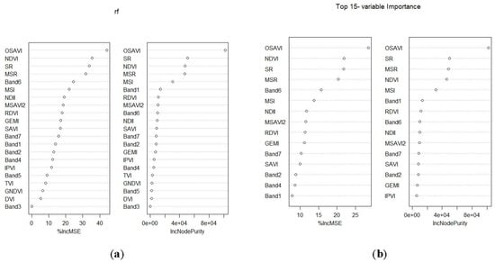
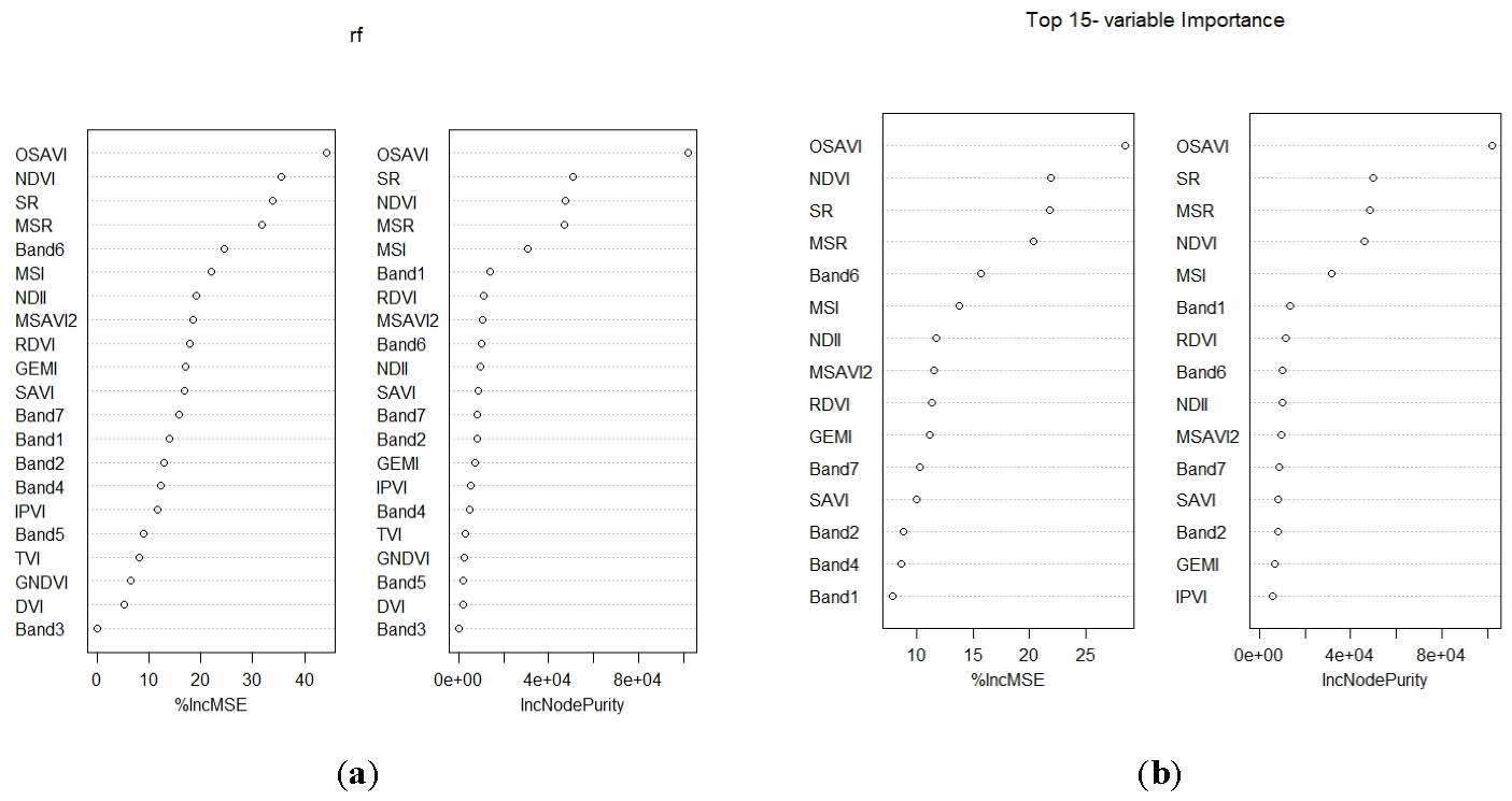
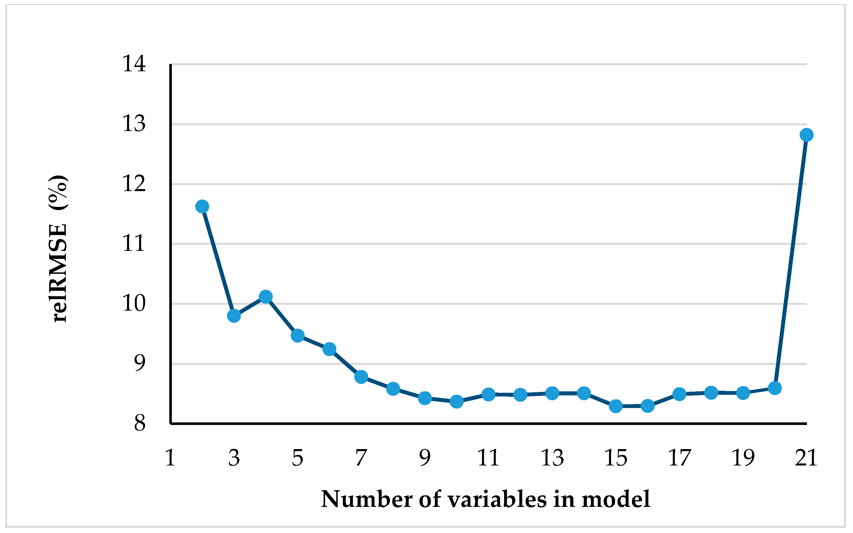
2.6.3. Variable Selection using Random Forest

One advantage of using the RF algorithm over other machine-learning algorithms is that it accomplishes excellent feature selection by automatically ranking the relative importance of the variables. The ranking is generated from out-of-bag (OOB) sample data. There are two mechanisms used in this algorithm to evaluate the importance of input variables (relevance of the predictor variables), assigning a score that depends on changes in the error when a particular variable is varied (%IncMSE refers to the effect of the variable when it is removed from the model, and IncNodePurity describes how pure the node is when that variable is in the model) [52]. Taking this into account, it was a challenging task to select the smallest number of predictor variables that could produce a good predictive power and thus helped to generate the final model. RF model using all independent variables was obtained by tuning ntree to 2000, whereas mtry was kept at 20. From a variable importance graph generated from the OOB data, we used a backward feature elimination method; this process uses the total variables used in the model (n = 21) and then progressively eliminates the least promising variables from the model. The permuted OOB data (nPerm) was iterated to assess the variable importance. For each iteration, the model is optimized (tuned) by selecting the best mtry and ntree and eliminating the variable that is the least important. The RMSE is then calculated. The tuning of ntree was set from 500 to 2000 with increments of 100, whereas mtry was tested in increments of 1 to 21. The subset of variables with the smallest RMSE values was used to predict the AGB of the selected community forest.

2.6.4. The Effectiveness of MLR and RF in Predicting the AGB of BZCFs

To evaluate the effectiveness of the MLR, the adjusted R2 value was considered as well as the cross-validation of the error terms. The pseudo R2 generated by the RF algorithm was not considered, thus the same cross-validation approach was used to examine the model performances. In this study, we used the 10-fold cross-validation method mainly because the original data is randomly divided into k equally sized (10) subsamples. A single subsample was retained as the validation data for testing the model, and the remaining k − 1 subsamples were then used in model training. This process is repeated for k times. One advantage of this method is that all the observations or assumptions are used for both training and validation. In addition, validation measures (Equations 2–4), namely R2, RMSE, relative RMSE (relRMSE), and coefficient of variance of the root mean square error (RMSE-CV) between the simulated AGB and the field-measured AGB, were calculated to assess the model‘s estimation performance. The method measures the percentage variation explained by the regression model [4].
  RMSE = i = 1 n ( y i   y ^ i ) 2   n  
where yi is the field-measured biomass at plot i, y ^ i is the predicted biomass value, and n is the number of the plots.
  r e l R M S E = 100 × ( R M S E Y ¯ )  
where Y ¯ represents the mean AGB value from the field measurements.
  RMSE-CV = ( R M S E Y ¯ )  
where RMSE-CV is the coefficient of variance of the root mean square error; RMSE is the root mean square error, and Y ¯ is the mean of the observed values.

3. Results

3.1. Field-Based AGB Estimates

Forest stand variables (DBH and H) measured for each sampled tree and aggregated for every sampling plot were used to generate the biomass of each community forest (Table 3). Descriptive statistics show that the minimum AGB was 30.34 t ha−1 and the maximum AGB was 304.19 t ha−1 for the Shrijana and Jyamire BZCFs, respectively. The average AGB estimated for the Terai region of Nepal was 196.18 t ha−1 [15]. The overall average AGB was 159.61 t ha−1 for six forests which did not exceed the FRA/DFRS (Forest Resource Assessment/ Department of Forest Research and Survey) value [15]. Altogether, 34 species were recorded in the field, of which only 8 species were unknown. Although many species were recorded, there were only five dominant species, namely sal (Shorea robusta), red berry (Mallotus philippensis), axlewood (Anogeissus latifolia), duabanga (Duabanga grandiflora), jamun (Syzygium cumini), and chilla (Casearia graveolens), where sal dominated the whole study area.

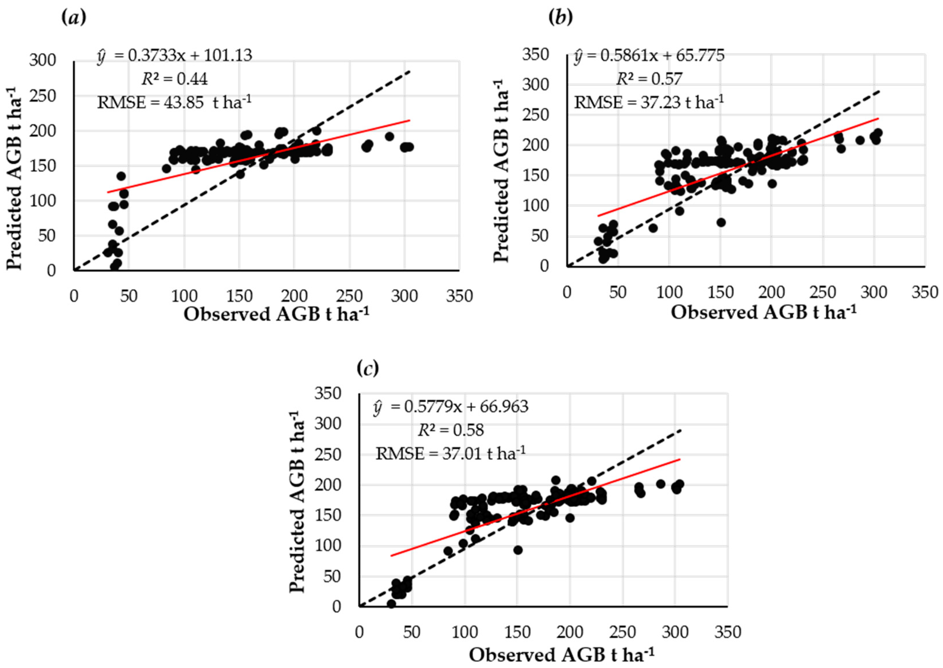
3.2. AGB Estimates using Landsat OLI Based on the MLR

AGB estimation results using Landsat 8-derived variables based on the MLR are shown in Table 4 and Figure 2. Multiple linear regression achieved moderate results when applied to the pooled dataset (ISI and VIs). For example, the pooled dataset as a predictor explained 56% of the variance (RMSE 37.01 t ha−1, relRMSE 23.05, p-value < 2.2 × 10⁻¹⁶) (Table 4 and Figure 2). The most important variables selected by the model were band 5 (NIR) and SR. Similarly, using VIs as predictor variables yielded more or less the same result, as it did for the combined dataset. No differences were seen in the adjusted R2 value, except for a slight change in RMSE (Adj. R2 = 0.56 and RMSE = 37.23 t ha−1). The selected predictor variables for the model were SR and MSI (statistically significant at the 95% level of confidence). In contrast, the use of spectral bands yielded the lowest adjusted R2, of 0.39, and the largest RMSE, of 43.85 t ha−1, and band 1 (Coastal), band 5 (NIR), and band 7 (SWIR2) were used as predictor variables in the final model.

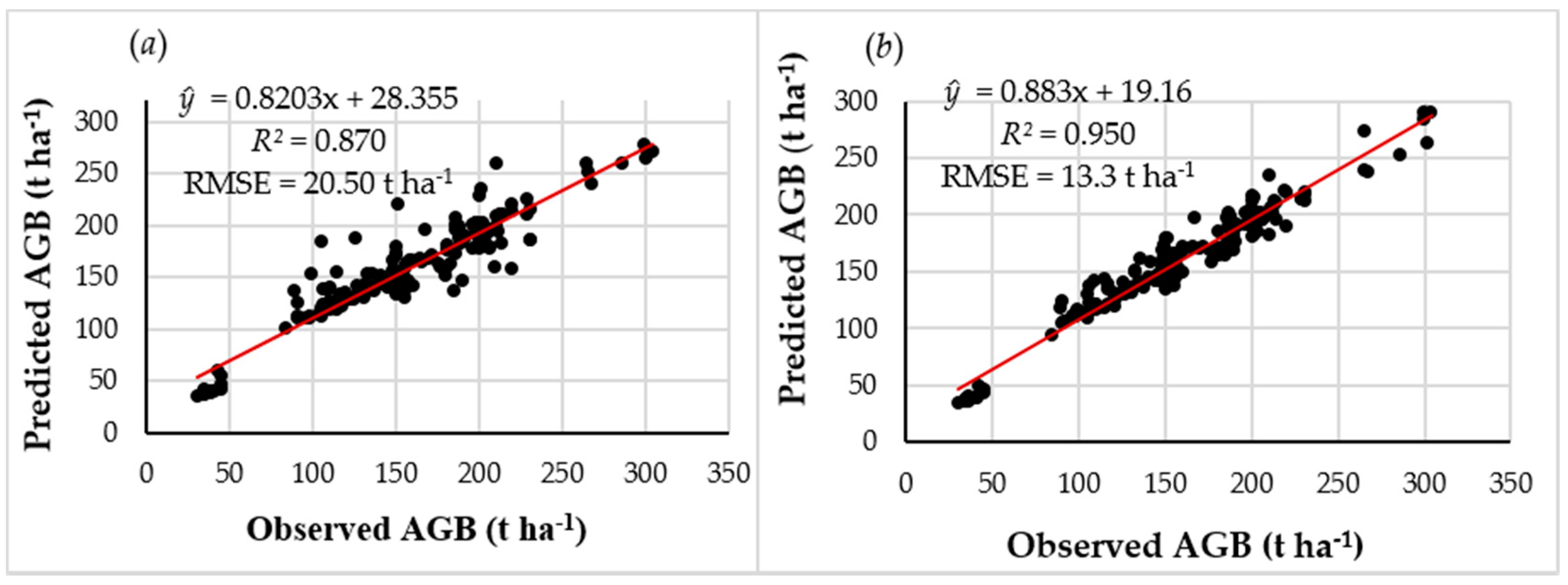
3.3. AGB Estimates using Pooled Data and Model Selected Predictor Variables Based on the RF Algorithm

Comparatively, the RF algorithm produced better AGB estimates using the combined dataset (ISI + VIs) as a full set of predictor variables (n = 21), as well as when the model selected variables were used. The use of the Landsat 8 OLI spectral information and the RF algorithm produced an R2 value of 0.870 and relRMSE of 12.82 when all predictor variables were used in the model. The backward variable selection resulted in a smaller, optimal number of important variables, producing an R2 of 0.95 and minimizing the relRMSE to 8.30 (Table 5 and Figure 3). The RMSE generally decreased as the least important variables were removed progressively from the RF model (Figure 4). Surprisingly, the results obtained from the use of the full set of predictor variables and those obtained using important selected variables did not differ. The same variables were identified as the important ones, but with different rankings based on the OOB (Figure 5).
When the RF algorithm with selected important variables (Figure 5) was used to predict AGB across six BZCFs, the result remained highly similar to those obtained using pooled data. The important variables selected were OSAVI, SR, MSR, NDVI, MSI, Band 1 (Coastal), RDVI, Band 6 (SWIR1), NDII, MSAVI2, Band 7 (SWIR2), SAVI, Band 2 (Blue), GEMI, and IPVI, in decreasing order of importance as selected by the OOB technique.

4. Discussion

The quantitative determination and mapping of forest AGB using remote-sensing techniques, especially with medium-resolution imagery, is quite a challenging task for complex and high-AGB forest stands. The use of multispectral sensors might be a good alternative for estimating AGB at the regional scale, especially in areas with limited access to hyperspectral images. Hyperspectral images are expensive and require advanced and unique technical expertise, making it challenging to determine estimation errors. In this study, we therefore tried to investigate whether the relatively new-generation Landsat 8 multispectral OLI has the capability to estimate the AGB of such complex forest, using two modeling approaches. The results have demonstrated that this spectrally enriched multispectral sensor offers invaluable opportunities, as it was capable of estimating AGB with presumably minimal errors. For instance, when extracted Landsat 8 OLI pooled data were used in the RF model, the R2 value reached 0.87 (n = 21), with RMSE = 20.50 t ha−1 and RMSE-CV = 0.13. This was also observed when using the MLR approach, where the combined data showed improved performance in estimating complex forest AGB, and this can be attributed to the sensor’s unique radiometric, spatial, and spectral characteristics, as reported in previous studies. Since the launch of Landsat 8 OLI, only a few studies have reported the potential use of this satellite data in estimating forest AGB [11,13]. For example, Karlson et al. [13] reported that the R2 based on seven Landsat 8 OLI images from 2013 to 2014 reached 0.57, with an RMSE of 17.6 t ha−1, for AGB in open woodlands in Burkina Faso. Similarly, Dube and Mutanga [41] showed the strength and performance of Landsat 8 OLI image-derived texture metrics in estimating the AGB of plantation forest in KwaZulu-Natal, South Africa. Many scholars have reported that Landsat sensors often dealt with the saturation problem of spectral bands as the biomass increases. For example, Steininger [53] observed saturation problems in an area with a biomass value above 150 t ha−1. In this study, we observed that this problem has been minimized, which can be attributed to the inclusion of the narrow or refined near-infrared bands. The NIR band minimizes the effect of water vapor absorption at a wavelength of 0.825 µm, thereby permitting accurate surface spectral detection, while minimizing satellite spectral saturation problems [54].
The above studies provided insights that corroborate the improvement made so far to the Landsat 8 OLI sensor. Some of these improvements can be attributed to the sensor’s push-broom scanning design, which is associated with an improved signal-to-noise ratio. Furthermore, the fine radiometric resolution of 12 bits makes the sensor more sensitive and robust in detecting crucial vegetation structural attributes [55,19]. In addition, a prolonged sensor radiation–sampling residence period for each field of view enhances the precision during spectral detection, and thus helps to minimize saturation problems. Thus, this unique sensor makes it a better alternative for landscape-scale biomass application than its predecessors and other costly sensors.
However, it is important to note that the improved AGB estimation model, obtained using pooled data from the 30-m Landsat 8 OLI multispectral sensor, can be linked to the strength of the advanced machine-learning algorithm of RF. In recent years, many scholars have successfully demonstrated the utility of the RF model in estimating forest AGB, and their findings are in line with ours. For example, Liu et al. [56] demonstrated that a RF AGB model showed the acceptable accuracy of R2 0.95 and RMSE = 17.73 Mg ha−1 when compared to the use of stepwise regression and support vector machine learning. Likewise, the study by Sadeghi et al. [57] also showed that the RF model can yield the best results for mapping boreal stand-level biomass (R2 = 0.62, RMSE = 26 Mg ha−1). Also, some authors have even reported that minimal AGB prediction error can be achieved using the RF technique. For instance, Latifi et al. [58] compared the performance of nearest-neighbor approaches, including RF, in predicting total volume and biomass at the plot level in a mixed temperate forest in southwestern Germany, using three different sets of remote-sensing data (aerial orthoimages, TM, and small-footprint LiDAR). They found that the RF model was superior to other nonparametric approaches.
In our study, the strength of the RF model was also examined based on an important variable selection technique, achieved through the model tuning process. In this study, the parameter tuning proved to be beneficial in AGB estimation using the RF model. For instance, the coefficient of determination increased from 0.87 to 0.95 and the RMSE decreased from 20.50 to 13.30 t ha−1. This observed result was surprising, as one would expect that the removal of less-important variables would not impact the model’s performance, as indicated by Kuhn et al. [59]. This presumably brings difficulties in understanding its computation, due to the complexity of the RF algorithm [60]. However, the advantages of using the RF model is that it offers the smallest subset of the input variables, which further optimizes the model’s performance through the OOB technique. The RF model provides an OOB data-based unbiased estimation error for the test dataset [61]. Performance of the algorithm depends on the selected parameters, such as the number of trees [52,62], splitting at each node of each tree [63,60], and the number of examples in each cell, below which the cell is not split [38], but equals the default value of the nodesize [64]. In this study, the default value was used as recommended in the literature. One limiting factor of random forest variables is that they do not automatically select the optimal number of variables that have the lowest error [65]. The empirical investigation by Grömping [62] showed that the choice of mtry in the RF model can substantially affect the allocated variable importance. Furthermore, the author stated that for the purposes of identifying a small number of variables sufficient for a good prediction, there is a need to avoid redundancy and obtain a parsimonious model. It is, therefore, not so important that the model contains all the relevant variables, as long as the prediction works well. In concordance with the authors of [62], in this study, the RF model identified 15 input variables as the smallest subset with satisfactory predictive ability.
The use of percentIncMSE and IncNodePurity (Figure 5) in ranking predictor variables in relation to their capability to predict forest AGB improved the model’s predictive accuracy. Although we achieved an acceptable result in this study, it is important to note that the performance of the model depends on the selection of important variables, such as the number of trees [52] and the number of splits. Kuhn and Johnson [59] suggested the use of at least 1000 trees for optimal RF model parameterization. Similarly, as suggested by Verikas et al. [61], using the optimal number of variables to split a node, instead of using a default value, results in different variable rankings. NDVI was ranked 4th mainly due to the presence of Landsat 8 OLI spectral saturation problems for high biomass [4], but the results showed that VIs better relate to AGB than spectral bands [54]. OSAVI could have been affected through the radiometric correction technique used to minimize the background effect (soil) in retrieving vegetation information [66,67]. Similarly, SR being the second most important variable selected reveals the presence of a dense canopy [68]. Using the Landsat 8 OLI sensor, the study by Shao and Zhang [69] showed that similar variables were selected for estimating forest biomass for coniferous and broad-leaved species in China.
Another possible explanation for the better performance in estimating AGB can be attributed to the ability of the RF to block the influence of noisy predictor variables [70]. The majority of the variables selected were from vegetation indices, and this might be one possible reason for the improved performance. Lu et al. [71] stated that the use of VIs can partially reduce the impacts of environmental conditions and shadows on reflectance, thus improving the correlation between AGB and VIs, especially in sites with complex vegetation stand structures. In addition, we attributed the strong performance of RF in this study to the collection of a sufficient reference dataset which contained a modest amount of extreme values. The extreme values were represented in the tree construction, and RF prediction was not biased towards the mean value [13]. Nevertheless, variables’ importance measures in this high-dimensional setting should be interpreted with care due to data redundancy. For example, collinearity among the predictors was not considered in the model. However, 45% of all the pairwise Pearson’s correlations among the predictors had values > 80, indicating high collinearity among the multiple predictors. Nevertheless, the good model parameter optimization minimized model overfitting problems and multicollinearity effects [61].
Although the objective of this study was not to compare algorithms, we also checked how well the RF model could estimate AGB in complex stands by comparing it to the MLR. Our result showed that the MLR performance was moderately satisfactory in predicting AGB. However, comparatively, the results were very weak when compared to the RF model observed AGB estimates. For instance, linear regression employed for the pooled dataset yielded an adjusted R2 of 0.56 (RMSE = 23.05 t ha−1) and identified the two most important variables as being Band 5 (NIR) and SR. Variable selection in the RF model yielded a similar result, except for that a different vegetation index (SAVI) was selected when compared to the MLR. The presence of multicollinearity was tested using the VIF, and those with a high value were removed from the model. The following variables, Bands 2, 3, 4, and 6; MSR; NDVI; RDVI; and MSAVI2, experienced high collinearity. As a result, the removal of highly collinear variables resulted in different variables being selected by the model. Similar results were observed for the other two datasets. In addition, it is important to note that the integration of the spectral bands and vegetation indices did not influence the model performance much (i.e., gave a slight improvement in the error term, but the same adjusted R2 value). On the other hand, the use of spectral bands as independent variables yielded weaker AGB estimates. This observation is not unique, but is in line with other studies where VIs were found to relate better with AGB than spectral bands [4,11,41]. For example, the study by Dube and Mutanga [11] used spectral bands and VIs to estimate commercial forest species’ (E. dunii, E. grandis, and P. taeda) biomass. The results showed that the spectral bands yielded an R2 of 0.40 (RMSE 18.13t ha−1), 0.32 (RMSE 29.13 t ha−1), and 0.30 (32.83 t ha−1), whereas VIs produced an R2 of 0.53 (RMSE 18.66 t ha−1), 0.36 (RMSE 26.54 t ha−1), and 0.37 (RMSE 29.48 t ha−1) for these three species, respectively.
The observed 56% model variability is comparable to previous findings in the literature [72]. Kumar et al. [72] obtained a lower AGB prediction accuracy of 0.44 using 250-m spatial resolution MODIS data. However, the MLR results are weak when compared to those of Zheng et al. [73], who obtained a high R2 of 0.82 in the simple-structured temperate forest. The previous studies in complex and dense forest obtained considerably lower results similar to those obtained in this study using the simple linear model [74,4,75,53].
Although we obtained a better AGB model, using vegetation indices, the MLR model explained half of the variability in biomass. Moreover, the RMSE of 37.01 t ha−1 obtained from cross-validation is still large, depicting model underestimation and overestimation for low and high biomass, respectively, within the study area. This could be due to an increase in homogenous texture and the higher prevalence of subtropical species in the study area (Figure 2). Very few plots were fitted on the line, suggesting that linear regression might not be suitable for AGB estimation in such complex and dense forests. However, the weak performance of MLR in AGB estimation in the complex forest ecosystem shows that the use of nonlinear models such as RF or SVM (support vector machine) [62] is critical if accurate estimates are to be obtained in such areas. It is important to note that there are various AGB modeling approaches using different sensors and in situ data. It is thus difficult to conclude outright that one model is more suitable than the other, until and unless they are assessed separately. This is only the way that different results can be shown when considering different forest types, sensors used, and topographical structures. Nevertheless, uncertainties in remote sensing techniques of AGB are high due to the structural variation of vegetation, heterogeneity of landscapes, seasonal variation, and disproportionate data availability, among others [76]. Since our study area lies in flat terrain and comprises almost homogenous canopy structures with high biomass, the potential of such a valuable sensor in AGB estimation in different forest environments with complex terrain can be exploited further, which can help to fill the voids related to the lack of data on forest resources.

5. Conclusions

Here, we investigated the utility of Landsat 8 OLI spectrally derived variables in estimating complex forest stand AGB based on two statistical analysis techniques, namely RF and MLR.
We concluded that:
  • Improvements in the medium-resolution Landsat 8 OLI have the potential to satisfactorily predict biomass in subtropical forest areas exhibiting flat terrain but complex forest characteristics.
  • Important variables’ selection from pooled data derived from Landsat 8 OLI using the RF model yielded better results with the lowest observed RMSE value when compared to the MLR model.
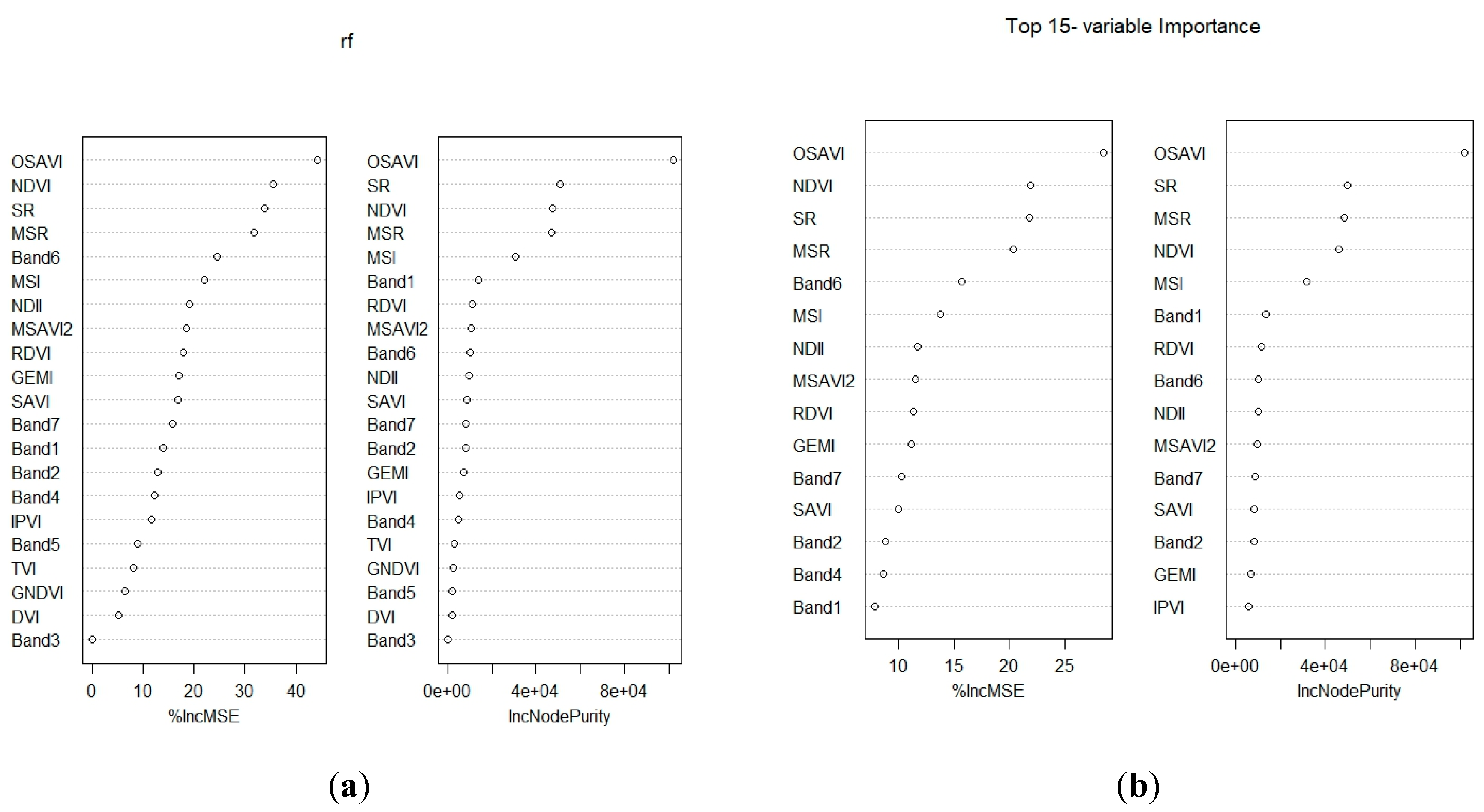
  • The RF model selected the Landsat 8 OLI-derived OSAVI, SR, and MSR as the most suitable variables for estimating AGB, whereas MLR selected Band 5 (NIR) and SR.
Overall, our results demonstrate the utility, potential, and strength of the combination in situ data with Landsat 8 OLI derivatives in predicting biomass. The method presented here is relatively simple and is applicable to other parts of Nepal, where access to hyperspectral data is limited. It should be a good alternative for researchers and conservationists who require cheap, efficient, and freely available satellite sensor data to use for the reliable and accurate monitoring of AGB and carbon sequestration where ground data are scarce. Furthermore, it can be utilized in strategic forest management in Nepal.

Author Contributions

S.P. designed the study, analyzed the data, and wrote the paper. S.T. and T.D. helped to review the manuscript.

Funding

This research received no external funding.

Acknowledgments

This study used some data from the Parsa National Park. We thank the Department of National Park and Wildlife Conservation, Nepal, for granting us with the permit to conduct field surveys. The Community Forest User’s Group, Forest guards, local members, and Amrit Science Campus are thanked for their kind support and assistance during the field phase. We thank Cletah Shoko from the University of KwaZulu-Natal for English editing of the final version of the manuscript. In addition, we thank the Editors and anonymous reviewers for their valuable comments and insightful suggestions.

Conflicts of Interest

The authors declare no conflict of interest.

References

  1. Ebregt, A.; Greve, P.D. Buffer Zones and Their Management: Policy and Best Practices for Terrestrial Ecosystems in Developing Countries; Theme Studies Series; National Reference Centre for Nature Management: Wageningen, The Netherlands, 2000. [Google Scholar]
  2. Stræde, S.; Treue, T. Beyond buffer zone protection: A comparative study of park and buffer zone products’ importance to villagers living inside Royal Chitwan National Park and to villagers living in its buffer zone. J. Environ. Manag. 2006, 78, 251–267. [Google Scholar] [CrossRef] [PubMed]
  3. Baral, S. Mapping Carbon Stock Using High-Resolution Satellite Images in the Sub-Tropical Forest of Nepal. Master’s Thesis, University of Twente, Enschede, The Netherlands, 2011. [Google Scholar]
  4. Lu, D. Aboveground biomass estimation using Landsat TM data in the Brazilian Amazon. Int. J. Remote Sens. 2005, 26, 2509–2525. [Google Scholar] [CrossRef]
  5. Patenaude, G.; Milne, R.; Dawson, T.P. Synthesis of remote sensing approaches for forest carbon estimation: Reporting to the Kyoto Protocol. Environ. Science Policy 2005, 8, 161–178. [Google Scholar] [CrossRef]
  6. Clark, M.L.; Roberts, D.A.; Ewel, J.J.; Clark, D.B. Estimation of tropical rain forest aboveground biomass with small-footprint lidar and hyperspectral sensors. Remote Sens. Environ. 2011, 115, 2931–2942. [Google Scholar] [CrossRef]
  7. Chen, J.; Gu, S.; Shen, M.; Tang, M.; Matsushita, B. Estimating aboveground biomass of grassland having a high canopy cover: An exploratory analysis of in situ hyperspectral data. Int. J. Remote Sens. 2009, 30, 6497–6517. [Google Scholar] [CrossRef]
  8. Dube, T.; Mutanga, O.; Abdel-Rahman, E.M. Predicting Eucalyptus spp. stand volume in Zululand, South Africa: an analysis using a stochastic gradient boosting regression ensemble with multi-source data sets. Int. J. Remote Sens. 2015, 36, 3751–3772. [Google Scholar] [CrossRef]
  9. Mutanga, O.; Adam, E.; Cho, M.A. High-density biomass estimation for wetland vegetation using Worldview-2 imagery and random forest regression algorithm. Int. J. Appl. Earth Obs. Geoinf. 2012, 18, 399–406. [Google Scholar] [CrossRef]
  10. Rana, P.; Korhonen, L.; Gautam, B.; Tokola, T. Effect of field plot location on estimating tropical forest above ground biomass in Nepal using airborne laser scanning data. ISPRS J. Photogramm. Remote Sens. 2014, 94, 55–62. [Google Scholar] [CrossRef]
  11. Dube, T.; Mutanga, O. Evaluating the utility of the medium-spatial resolution Landsat 8 multi-spectral sensor in quantifying aboveground biomass in Umgeni catchment, South Africa. ISPRS J. Photogramm. Remote Sens. 2015, 101, 36–46. [Google Scholar] [CrossRef]
  12. Mathieu, R.; Naidoo, L.; Cho, M.A.; Leblon, B.; Main, R.; Wessels, K.; Asner, G.P.; Buckely, J.; Aardt, J.V.; Erasmus, B.F.N.; et al. Toward structural assessment of semi-arid African savannahs and woodlands: The potential of multitemporal polarimetric RADARSAT-2 fine beam images. Remote Sens. Environ. 2013, 138, 215–231. [Google Scholar] [CrossRef]
  13. Karlson, M.; Ostwald, M.; Reese, H.; Sanou, J.; Tankoano, B.; Mattsson, E. Mapping tree canopy cover and aboveground biomass in Sudano-Sahelian Woodlands using Landsat 8 and Random forest. Remote Sens. 2015, 7, 10017–10041. [Google Scholar] [CrossRef]
  14. Karna, Y.K.; Hussin, Y.A.; Gilani, H.; Bronsveld, M.C.; Murthy, M.S.R.; Qamer, F.M.; Karky, B.S.; Bhattarai, T.; Aigong, X.; Baniya, C.B. Integration of WorldView-2 and airborne LiDAR data for tree species level carbon stock mapping in Kayar Khola watershed, Nepal. Int. J. Appl. Earth Obs. Geoinf. 2015, 38, 280–291. [Google Scholar] [CrossRef]
  15. FRA/DFRS. Terai Forests of Nepal (2010-2012); Forest Resource Assessment Nepal/Department of Forest Research and Survey: Babarmahal, Kathmandu, Nepal, 2014. [Google Scholar]
  16. Murthy, M.S.R.; Wesselman, S.; Gilani, H. Multi-Scale Forest Biomass Assessment and Monitoring in the Hindu Kush Himalayan Region: A Geospatial Perspective; International Centre for Integrated Mountain Development (ICIMOD): Kathmandu, Nepal, 2015; pp. 70–82. [Google Scholar]
  17. Muinonen, E.; Parikka, H.; Pokharel, Y.P.; Shrestha, S.M.; Eerikäinen, K. Utilizing a multi-source forest inventory technique, MODIS data and Landsat TM images in the production of forest cover and volume maps for the Terai Physiographic Zone in Nepal. Remote Sens. 2012, 4, 3920–3947. [Google Scholar] [CrossRef]
  18. Koju, U.; Zhang, J.; Gilani, H. Exploring multi-scale forest above ground biomass estimation with optical remote sensing imageries. IOP Conf. Ser. Earth Environ. Sci. 2017, 57, 012011. [Google Scholar] [CrossRef] [Green Version]
  19. Pahlevan, N.; Schott, J.R. Leveraging EO-1 to evaluate capability of new generation of Landsat sensors for Coastal/Inland water studies. IEEE J. Sel. Top. Appl. Earth Obs. Remote Sens. 2013, 6, 360–374. [Google Scholar] [CrossRef]
  20. Irons, J.R.; Dwyer, J.L.; Barsi, J.A. The next Landsat satellite: The Satellite data continuity mission. Remote Sens. Environ. 2012, 122, 11–21. [Google Scholar] [CrossRef]
  21. Zhao, P.; Lu, D.; Wang, G.; Wu, C.; Huang, Y.; Yu, S. Examining spectral reflectance saturation in Landsat Imagery and corresponding solution to improve forest aboveground biomass estimation. Remote Sens. 2016, 8, 469. [Google Scholar] [CrossRef]
  22. Chave, J.; Andalo, C.; Brown, S.; Cairns, M.A.; Chambers, J.Q.; Eamus, D.; Fölster, H.; Fromard, F.; Higuchi, N.; Kira, T.; et al. Tree allometry and improved estimation of carbon stocks and balance of tropical forest. Ecosyst. Ecol. 2005, 145, 87–99. [Google Scholar] [CrossRef] [PubMed]
  23. ANSAB; FECOFUN; ICIMOD. Forest Carbon Stock Measurement: Guidelines for Measuring Carbon Stocks in Community-Managed Forests; Asia Network for Sustainable Agriculture and Bioresources (ANSAB), International Centre for Integrated Mountain Development (ICIMOD), and Federation of Community Forest Users, Nepal (FECOFUN): Kathmandu, Nepal, 2010. [Google Scholar]
  24. Chaturvedi, A.N.; Khanna, L.S. Forest Mensuration; International Book Distributors: Dehra Dun, India, 1982. [Google Scholar]
  25. Dube, T. Primary Productivity of Intertidal Mudflats in the Wadden Sea: A Remote Sensing Method. Master’s Thesis, University of Twente, Enschede, The Netherlands, 2012. [Google Scholar]
  26. Dube, T.; Mutanga, O.; Elhadi, A.; Ismail, R. Intra-and-inter species biomass prediction in a plantation forest: Testing the utility of high spatial resolution space borne multispectral RapidEye sensor and advance machine learning algorithms. Sensors 2014, 14, 15348–15370. [Google Scholar] [CrossRef] [PubMed]
  27. Huete, A.R. A soil-adjusted vegetation index (SAVI). Remote Sens. Environ. 1988, 25, 295–309. [Google Scholar] [CrossRef]
  28. Rouse, J.W., Jr. Monitoring the Vernal Advancement and Retrogra-Dation (Green wave Effect) of Natural Vegetation; NASA/GSFC: Washington, DC, USA, 1974. [Google Scholar]
  29. Jordan, C.F. Derivation of leaf-area index from quality of light on the forest floor. Ecology 1969, 50, 663–666. [Google Scholar] [CrossRef]
  30. Qi, J.; Chehbouni, A.; Huete, A.R.; Kerr, Y.H.; Sorooshian, S. A modified soil adjusted vegetation index. Remote Sens. Environ. 1994, 48, 119–126. [Google Scholar] [CrossRef]
  31. Hunt, E.R., Jr.; Rock, B.N. Detection of changes in leaf water content using near-and middle-infrared reflectances. Remote Sens. Environ. 1989, 30, 43–54. [Google Scholar] [CrossRef]
  32. Hardisky, M.A.; Klemas, V.; Smart, R.M. The influence of soil salinity, growth form, and leaf moisture on the spectral radiance of Spartina alterniflora canopies. Photogramm. Eng. Remote Sens. 1983, 49, 77–83. [Google Scholar]
  33. Pinty, B.; Verstraete, M.M. GEMI: A non-linear index to monitor global vegetation from satellites. Plant Ecol. 1992, 101, 15–20. [Google Scholar] [CrossRef]
  34. Roujean, J.L.; Breon, F.M. Estimating PAR absorbed by vegetation from bidirectional reflectance measurements. Remote Sens. Environ. 1995, 51, 375–384. [Google Scholar] [CrossRef]
  35. R Development Core Team. R: A Language and Environment for Statistical Computing; R Foundation for Statistical Computing: Vienna, Austria, 2015. [Google Scholar]
  36. Davison, A.C.; Hinkley, D.V. Bootstrap Methods and Their Applications; Cambridge University Press: Cambridge, UK, 1997; ISBN 0-521-57391-2. [Google Scholar]
  37. Faraway, J.J. Practical Regression and ANOVA Using R; University of Michigan: Ann Arbor, MI, USA, 2002. [Google Scholar]
  38. Kuhn, M. Building Predictive Models in R Using the caret Package. J. Stat. Softw. 2008, 28, 1–26. [Google Scholar] [CrossRef]
  39. Liaw, A.; Matthew, W. Classification and regression by randomforest. R News 2002, 2, 18–22. [Google Scholar]
  40. Fassnacht, F.E.; Hartig, F.; Latifi, H.; Berger, C.; Hernández, J.; Corvalán, P.; Koch, B. Importance of sample size, data type and prediction method for remote sensing-based estimations of aboveground forest biomass. Remote Sens. Environ. 2014, 154, 102–114. [Google Scholar] [CrossRef]
  41. Dube, T.; Mutanga, O. Investigating the robustness of the newly Landsat-8 Operational Land Imager derived texture metrics in estimating plantation forest aboveground biomass in resource constrained areas. ISPRS J. Photogramm. Remote Sens. 2015, 108, 12–32. [Google Scholar] [CrossRef]
  42. Peat, J.; Barton, B. Medical Statistics: A Guide to Data Analysis and Critical Appraisal; John Wiley & Sons: Hoboken, NJ, USA, 2008. [Google Scholar]
  43. Öztuna, D.; Elhan, A.H.; Tüccar, E. Investigation of four different normality tests in terms of type 1 error rate and power under different distributions. Turkish J. Med. Sci. 2006, 36, 171–176. [Google Scholar]
  44. Dye, M.; Mutanga, O.; Ismail, R. Examining the utility of random forest and AISA Eagle hyperspectral image data to predict Pinus patula age in KwaZulu-Natal, South Africa. Geocarto Int. 2011, 26, 275–289. [Google Scholar] [CrossRef]
  45. Ismail, R.; Mutanga, O. A comparison of regression ensembles: Predicting Sirex noctilio induced water stress in Pinus patula forest of KwaZulu-Natal, South Africa. Int. J. App. Earth Obs. Geoinf. 2010, 12, S45–S51. [Google Scholar] [CrossRef]
  46. Prasad, A.M.; Iverson, L.R.; Liaw, A. Newer Classification and Regression Tree Techniques: Bagging and Random Forests for Ecological Prediction. Ecosystems 2006, 9, 181–199. [Google Scholar] [CrossRef]
  47. Breiman, L. Random forests. Mach. Learn. 2001, 45, 5–32. [Google Scholar] [CrossRef]
  48. Ozcift, A. Random forest ensemble classifier trained with data resampling strategy to improve cardiac arrhythmia diagnosis. Comput. Biol. Med. 2011, 41, 265–271. [Google Scholar] [CrossRef] [PubMed]
  49. Palmer, D.S.; O’Boyle, N.M.; Glen, R.C.; Mitchell, J.B.O. Random forest model to predict aqueous solubility. J. Chem. Inf. Model. 2007, 47, 150–158. [Google Scholar] [CrossRef] [PubMed]
  50. Probst, P.; Boulesteix, A.L. To tune or not to tune the number of trees in random forest. J. Mach. Learn. Res. 2018, 18, 1–18. [Google Scholar]
  51. Scornet, E.; Biau, G.; Vert, J.P. Consistency of random forests. Ann. Stat. 2015, 43, 1716–1741. [Google Scholar] [CrossRef] [Green Version]
  52. Genuer, R.; Poggi, J.M.; Tuleau-Malot, C. Variable selection using random forests. Pattern Recognit. Lett. 2010, 31, 2225–2236. [Google Scholar] [CrossRef] [Green Version]
  53. Steininger, M.K. Satellite estimation of tropical secondary forest above-ground biomass: Data from Brazil and Bolivia. Int. J. Remote Sens. 2000, 21, 1139–1157. [Google Scholar] [CrossRef] [Green Version]
  54. Lu, D. The potential and challenges of remote sensing-based biomass estimation. Int. J. Remote Sens. 2006, 27, 1297–1328. [Google Scholar] [CrossRef]
  55. El-Askary, H.; Abd El-Mawla, S.H.; Li, J.; El-Hattab, M.M.; El-Raey, M. Change detection of coral reef habitat using Landsat-5 TM, Landsat 7 ETM+ and Landsat 8 OLI data in the Red Sea (Hurghada, Egypt). Int. J. Remote Sens. 2014, 35, 2327–2346. [Google Scholar] [CrossRef]
  56. Liu, K.; Wang, J.; Zeng, W.; Song, J. Comparison and evaluation of three models for estimating forest above ground biomass using TM and GLAS data. Remote Sens. 2017, 9, 341. [Google Scholar] [CrossRef]
  57. Sadeghi, Y.; St-Onge, B.; Leblon, B.; Prieur, J.F.; Simard, M. Mapping boreal forest biomass from a SRTM and TanDEM-X based on canopy height model and Landsat spectral indices. Int. J. Appl. Earth Obs. Geoinf. 2018, 68, 202–213. [Google Scholar] [CrossRef]
  58. Latifi, H.; Nothdurft, A.; Koch, B. Non-parametric prediction and mapping of standing timber volume and biomass in a temperate forest: Application of multiple optical/LiDAR-derived predictors. Forestry 2010, 83, 395–407. [Google Scholar] [CrossRef]
  59. Kuhn, M.; Johnson, K. Applied Predictive Modeling; Springer: New York, NY, USA, 2013. [Google Scholar]
  60. Biau, G.; Scornet, E. A random forest guided tour. Test 2016, 25, 197–227. [Google Scholar] [CrossRef]
  61. Verikas, A.; Gelzinis, A.; Bacauskiene, M. Mining data with random forests: A survey and results of new tests. Pattern Recognit. 2011, 44, 330–349. [Google Scholar] [CrossRef]
  62. Oshiro, T.M.; Perez, P.S.; Baranauskas, J.A. How many trees in a random forest. In International Workshop on Machine Learning and Data Mining in Pattern Recognition; Springer: Berlin/Heidelberg, Germany, 2012. [Google Scholar]
  63. Grömping, U. Variable importance assessment in regression: Linear regression versus random forest. Am. Stat. 2009, 63, 308–319. [Google Scholar] [CrossRef]
  64. Tyralis, H.; Papacharalampous, G. Variable Selection in Time Series Forecasting Using Random Forests. Algorithms 2017, 10, 114. [Google Scholar] [CrossRef]
  65. Adam, E.M.; Mutanga, O.; Rugege, D.; Ismail, R. Discriminating the papyrus vegetation (Cyperus papyrus L.) and its co-existent species using random forest and hyperspectral data resampled to HYMAP. Int. J. Remote Sens. 2012, 33, 552–569. [Google Scholar] [CrossRef]
  66. Chen, J.M. Evaluation of Vegetation Indices and a Modified Simple Ratio for Boreal Applications. Can. J. Remote Sens. 1996, 22, 229–242. [Google Scholar] [CrossRef]
  67. Ojoyi, M.; Mutanga, O.; Odindi, J.; Abdel-Rahman, E.M. Application of topo-edaphic factors and remotely sensed vegetation indices to enhance biomass estimation in a heterogeneous landscape in the Eastern Arc Mountains of Tanzania. Geocarto Int. 2016, 31, 1–21. [Google Scholar] [CrossRef]
  68. Mutanga, O.; Skidmore, A.K. Narrow band vegetation indices overcome the saturation problem in biomass estimation. Int. J. Remote Sens. 2004, 25, 3999–4014. [Google Scholar] [CrossRef]
  69. Shao, Z.; Zhang, L. Estimating forest aboveground biomass by combining optical and SAR data: A case study in Genhe, Inner Mongolia, China. Sensors 2016, 16, 834. [Google Scholar] [CrossRef] [PubMed]
  70. Adam, E.M.; Mutanga, O.; Abdel-Rahman, E.M.; Ismail, R. Estimating standing biomass in papyrus (Cyperus papyrus L.) swamp: Exploratory of in situ hyperspectral indices and random forest regression. Int. J. Remote Sens. 2014, 35, 693–714. [Google Scholar] [CrossRef]
  71. Lu, D.; Mausel, P.; Brondızio, E.; Moran, E. Relationships between forest stand parameters and Landsat TM spectral responses in the Brazilian Amazon Basin. For. Ecol. Manag. 2004, 198, 149–167. [Google Scholar] [CrossRef] [Green Version]
  72. Kumar, R.; Gupta, S.R.; Singh, S.; Patil, P.; Dhadhwal, V.K. Spatial distribution of Forest biomass using remote sensing and regression models in Northern Haryana, India. Int. J. Ecol. Environ. Sci. 2011, 37, 37–47. [Google Scholar]
  73. Zheng, D.; Rademacher, J.; Chen, J.; Crow, T.; Bresee, M.; Le Moine, J.; Ryu, S.R. Estimating aboveground biomass using Landsat 7 ETM+ data across a managed landscape in northern Wisconsin, USA. Remote Sens. Environ. 2004, 93, 402–411. [Google Scholar] [CrossRef]
  74. Foody, G.M.; Cutler, M.E.; Mcmorrow, J.; Pelz, D.; Tangki, H.; Boyd, D.S.; Douglas, I. Mapping the biomass of Bornean tropical rain forest from remotely sensed data. Global Ecology and Biogeography 2001, 10, 379–387. [Google Scholar] [CrossRef]
  75. Rahman, M.M.; Csaplovics, E.; Koch, B. An efficient regression strategy for extracting forest biomass information from satellite sensor data. Int. J. Remote Sens. 2005, 26, 1511–1519. [Google Scholar] [CrossRef]
  76. Kumar, L.; Mutanga, O. Remote Sensing of Above-Ground Biomass. Remote Sens. 2017, 9, 935. [Google Scholar] [CrossRef]
Figure 1. Study area map showing the Parsa National Park (PNP) with buffer zone community forests (BZCFs) and sample plots.
Remotesensing 10 01848 g001
Figure 2. Observed vs predicted aboveground biomass (AGB) using an MLR approach for (a) image spectral information (ISI), (b) vegetation indices (VIs), and (c) ISI + VIs.
Remotesensing 10 01848 g002
Figure 3. Observed vs predicted aboveground biomass (t ha−1) using the RF algorithm and (a) pooled data and (b) only selected important variables.
Remotesensing 10 01848 g003
Figure 4. Relative RMSEs obtained by backward elimination of variables from the random forest model.
Remotesensing 10 01848 g004
Figure 5. (a) Important variable ranking by Random forest algorithm and (b) top 15 selected important variables.
Remotesensing 10 01848 g005
Table 1. Examined variables for the multiple linear regression (MLR) and random forest (RF) models.
Data TypeModelInput Variables
Image spectral information (ISI)MLRband 2 (BLUE), band 3 (GREEN), band 4 (RED), band 5 (NIR), band 6 (SWIR1), band 7 (SWIR2)
Vegetation indices (VIs)MLRDVI, GEMI, GNDVI, MSAVI2, MSI, NDII, NDVI, OSAVI, RDVI, MSR, SAVI, SR, TVI, and IPVI
ISI + VIs MLR/RFISI + DVI, GEMI, GNDVI, MSAVI2, MSI, NDII, NDVI, OSAVI, RDVI, MSR, SAVI, SR, TVI, and IPVI
Most important variablesRFOSAVI, NDVI, SR, MSR, band 6, MSI, NDII, MSAVI2, RDVI, GEMI, band 7, SAVI , band 2, band 4, and band 1
Most importantvariables MLRband 5 and SR (pooled data), SR and MSI (VIs), and band 1, band 5, and band 7
NIR: near-infrared; SWIR1: short-wave infrared 1; SWIR2: short-wave infrared 2; DVI: difference vegetation index; GEMI: global environmental monitoring index; GNDVI: green normalized difference vegetation index; MSAVI2: second modified soil-adjusted vegetation index; MSI: moisture stress index; NDII: normalized difference infrared index; NDVI: normalized difference vegetation index; OSAVI: optimized soil-adjusted vegetation index; RDVI: renormalized difference vegetation index; MSR: modified simple ratio; SAVI: soil-adjusted vegetation index; SR: simple ratio; TVI: triangular vegetation index; IPVI: infrared percentage vegetation index.
Table 2. Important image spectral information and vegetation indices selected for the RF model.
Band reflectance usedBlue, Red, SWIR1, SWIR2
Vegetation indicesFormulaReferences
Optimized soil-adjusted vegetation index (OSAVI)[(NIR − RED) / (NIR + RED + L)] × (1 + L), where L = 0.16 and is the soil brightness correction factor[27]
Normalized difference vegetation index (NDVI)(NIR − RED) / (NIR + RED)[28]
Simple ratio (SR)NIR/RED[29]
Modified simple ratio (MSR)(NIR / RED) − 1 / √((NIR / RED)) + 1 [30]
Moisture stress index (MSI)ꝭ1599 µm / ꝭ819 µm, where ꝭ = wavelength, Band 5 = 819 µm, Band 6 µm = 1599[31]
Normalized difference infrared index (NDII)(ꝭ819 µm − ꝭ1649 µm) / (ꝭ819 µm + ꝭ1649 µm), where Band 5 = 819 µm, Band 6 = 1599 µm[32]
Global environmental monitoring index (GEMI)n × (1 − 0.25 n) − [(RED − 0.125) / (1 − RED), where n = [2 × (NIR2 − RED2) + 1.5 × NIR + 0.5 × RED] / (NIR + RED + 0.5)[33]
Second modified soil-adjusted vegetation index (MSAVI2)1/2 × ((NIR + 1) − sqrt ((2 × NIR+ 1)2 − 8(NIR − RED)))[30]
Renormalized difference vegetation index (RDVI)(NDVI × DVI)0.5[34]
Soil-adjusted vegetation index (SAVI)(NIR − RED) / (NIR + RED + L) × (1 + L), where L = 0.5[27]
Table 3. Descriptive statistics of plot-level aboveground biomass (AGB).
No.Name of ForestTotal No. of PlotsMin(t ha−1)Max(t ha−1)Mean(t ha−1)Standard Deviation
1Ratomate Deurali BZCF1735.25115.95115.8733.66
2Jyamire BZCF3034.75304.19166.8188.60
3Radha Krishna BZCF59105.40230.72174.9135.51
4Janahit BZCF3096.95286.56172.1847.32
5Shrijana BZCF2130.34200.22117.9456.33
6Mushaharnimae BZCF1690.95210.48170.5240.26
Table 4. Biomass prediction results based on the MLR.
Cross-Validation
Final Variable Inputs in the ModelR2Adj. R2RMSE (t ha−1)relRMSE (%)RMSE-CV
Band 1, band 5, and band 70.410.3943.8527.420.27
SR and MSI0.570.5637.2323.080.23
Band 5 and SR0.560.5637.0123.050.23
relRMSE: relative root mean square error, RMSE-CV: coefficient of variance of the root mean square error.
Table 5. Biomass prediction results based on the RF.
Final Variable Inputs in the ModelModelR2RMSE (t ha-1)relRMSE (%)RMSE-CV
All variables (Table 1)RF (n = 21)0.8720.5012.820.13
See Table 2RF (selected variables)0.9513.308.300.08

