Article

Spatial Consistency Assessments for Global Land-Cover Datasets: A Comparison among GLC2000, CCI LC, MCD12, GLOBCOVER and GLCNMO

1
State Key Laboratory of Earth Surface Processes and Resource Ecology, Faculty of Geographical Science, Beijing Normal University, Beijing 100875, China
2
Institute of Land Surface System and Sustainable Development, Faculty of Geographical Science, Beijing Normal University, Beijing 100875, China
*
Author to whom correspondence should be addressed.
Remote Sens. 2018, 10(11), 1846; https://doi.org/10.3390/rs10111846
Submission received: 27 September 2018 / Revised: 11 November 2018 / Accepted: 16 November 2018 / Published: 21 November 2018
(This article belongs to the Special Issue Recent Advances in Satellite Derived Global Land Product Validation)

Abstract

:
Numerous global-scale land-cover datasets have greatly contributed to the study of global environmental change and the sustainable management of natural resources. However, land-cover datasets inevitably experience information loss because of the nature of the uncertainty in the interpretation of remote-sensing images. Therefore, analyzing the spatial consistency of multi-source land-cover datasets on the global scale is important to maintain the consistency of time and consider the effects of land-cover changes on spatial consistency. In this study, we assess the spatial consistency of five land-cover datasets, namely, GLC2000, CCI LC, MCD12, GLOBCOVER and GLCNMO, at the global and continental scales through climate and elevation partitions. The influencing factors of surface conditions and data producers on the spatial inconsistency are discussed. The results show that the global overall consistency of the five datasets ranges from 49.2% to 67.63%. The spatial consistency of Europe is high, and the multi-year value is 66.57%. In addition, the overall consistency in the EF climatic zone is very high, around 95%. The surface conditions and data producers affect the spatial consistency of land-cover datasets to different degrees. CCI LC and GLCNMO (2013) have the highest overall consistencies on the global scale, reaching 67.63%. Generally, the consistency of these five global land-cover datasets is relatively low, increasing the difficulty of satisfying the needs of high-precision land-surface-process simulations.

Graphical Abstract

1. Introduction

LUCC (Land use and land cover change) is a cause and consequence of global environmental change [1,2]. Changes in land use and land cover greatly alter the ecological process and land resource management, i.e. energy fluxes of land surface, carbon sequestration, water balance, as well as land use policy decisions [3,4,5,6]. At the same time, land use/land cover change is one of the most essential inputs for many land-surface models and is the basis for spatial inferences [7,8,9,10,11]. Compared to traditional methods (e.g., field surveys), remote sensing can provide large-scale and long time-series information of the Earth’s surface [12]. The most commonly used global land-cover datasets included the Matthews, Olson and Watts, and the Wilson and Henderson-Sellers global databases before the 90s, which have trouble meeting the needs of the global-change science community for very coarse resolution (typically 1° latitude by 1° longitude) [13,14,15]. As early as 1995, the International Geosphere-Biosphere Programme (IGBP) and the International Human Dimensions Programme on Global Environmental Change (IHDP) jointly proposed the important issue of “land use and land cover change” (LUCC). The international community has been developing medium- and high-resolution land-cover data products on the global scale, and a series of land-cover datasets have been released. An upsurge in global land-cover mapping began after the launch of the National Oceanographic and Atmospheric Administration (NOAA) satellite with an Advanced Very High Resolution Radiometer (AVHRR) instrument [16]. Based on the above images, IGBP DISCover [17,18] depicted 1 km of land cover in 1992–1993. By using Medium Resolution Imaging Spectrometer (MERIS) images, the European Space Agency (ESA) initiated the development of two 300-m resolution datasets named the Global LC Map (GLOBCOVER) [19,20] and Climate Change Initiative LC dataset (CCI LC) [21]. According to the GLOBCOVER project’s experiences, CCI LC shows high stability, which is extremely important when the time series of LC datasets are required for model input [21].
The nature of remote-sensing interpretation mandates that uncertainty will permeate the entire process of obtaining, processing, analyzing and expressing the results of remote-sensing information. Land-cover datasets, which are the simulation and generalization of land-cover characteristics, also frequently experience the loss of information and errors [22,23,24,25,26]. Therefore, spatial consistency assessments for global land-cover datasets are important to provide some beneficial suggestions for use in future global land-cover mapping and to the users of these datasets for effectively applying these products to their specific applications. Many researchers have conducted accuracy evaluations for a large number of land datasets. Giri et al. found that the spatial consistency between GLC2000 and MODIS products has significant regional differences [27]. Mccallum found that the consistency among the IGBP DISCover, UMD, GLC2000 and MOD12 global land-cover datasets in Asia was very low by measuring agreement and disagreement with existing land-cover maps [28]. Armel et al. studied the consistency of four types of remote-sensing land products for the African continent, which ranged between 56% and 69% [29]. Latifovic et al. found that GLC2000 showed better agreement with the reference data in sub-arctic and arctic areas than the IGBP and BU land-cover maps [30]. Ran et al. found that GLC2000’s land-cover map had the highest accuracy in China among the IGBP, UMd, GLC2000 and MODIS land-cover maps [31]. Wu et al. found that the coarse spatial resolution, the use of the per-pixel classification approach, and landscape heterogeneity were the main reasons for these large discrepancies [32]. In short, high amounts of uncertainty and inconsistency, which may be caused by various differences in satellite platforms, satellite sensor types, data sources, classification technology methods and land-cover classification systems.
However, these researchers did not maintain temporal consistency to make cross-time comparisons, thus neglecting the effect of land-cover change on the spatial consistency. Driven by different factors such as tropical deforestation, agricultural expansion, agricultural expansion, population growth, and economic development, some land use types have greatly changed on global, continental and national scales [33,34,35]. In view of the great change, the cross-time comparisons for spatial consistency assessment for global land-cover datasets may be unreliable. Moreover, previous studies on spatial consistency mostly focused on administrative zoning (continental or national scales). In this regard, conducting consistency comparisons based on principles of temporal consistency and geographical zoning such as elevation and climatic zones should be more productive. On the one hand, making comparisons based on the temporal consistency can effectively reduce the effect of land-use change on the spatial consistency. On the other hand, we can detect the effects of spatial heterogeneity on the spatial consistency of land-cover datasets when spatial consistency studies are performed based on geographic partitions, such as elevation and climatic zones.
Thus, we adopt methods such as overall consistency and category consistency analysis to compare the spatial consistency of land-cover datasets, including the GLOBAL LC 2000 dataset (GLC2000) [36], CCI LC, Moderate Resolution Imaging Spectroradiometer LC dataset (MCD12) [37], GLOBCOVER and Global Map-Global LC dataset (GLCNMO) [38], based on the principle of temporal consistency. Our research goals are to (1) study the spatial consistency of multi-source data for the entire globe and individual continents and (2) identify spatially consistent gradient characteristics of datasets for elevation partitions and climatic zones.

2. Materials and Methods

2.1. Data Resources and Preprocessing

Before comparing the results, we must understand the similarities and differences among the following five datasets: (1) GLC2000 from the European Commission’s Joint Research Center (JRC); (2) MCD12, which is available at an annual scale from 2001 to 2013; (3) GLOBCOVER from the European Space Agency (ESA, 2005/2009); (4) CCI LC from the ESA, which is available at an annual scale from 1992 to 2015; and (5) GLCNMO from the International Steering Committee for Global Mapping (2003/2008/2013). The characteristics of these five land-cover datasets are summarized in Table 1.
The above land-cover datasets are extracted according to the boundaries of continents, climate zones and elevation partitions. The projection system of land-cover datasets after extraction is transformed to the continental-scale Albers equal-area projection. These five datasets range in resolution from 300 m to 1 km, so resampling is required for comparison analysis, and the spatial resolution is adjusted to 1 km by the nearest-neighbor method. Reclassification is the other important step because these five datasets have different classification schemes. For example, GLOBCOVER (2005/2009) uses FAO LCCS classification schemes with 22 classes and MCD12 uses IGBP classification scheme with 17 classes. To facilitate the comparison, the initial classification code must be normalized, and detailed land-cover objects are required to merge and form a set of unified and generalized conversion criteria. The conversion relationship between the original schemes of the land-cover datasets and the target scheme is provided in Table 2. Additionally, the ocean and Antarctica are not considered in this comparison. All the land-cover datasets are converted into a consistent classification system with nine types (see Table 2).
Furthermore, DEM data uses resampled data with 1-km resolution from the SRTM 90-m Digital Elevation Database v4.1, and climate-zone data are reclassified based on world maps of KÖPPEN-GEIGER climate classification [44].

2.2. Analysis Methods

2.2.1. Category Composition Similarity Analysis

For each dataset, we count and summarize the area of each land-cover type and calculate the correlation coefficient of area series between each dataset, which evaluates the similarity of the land-cover datasets’ quantitative composition and Hu also conducted category composition similarity analysis in Europe for GLOBCOVER2005, GLOBCOVER2009, GLC2000 and MODIS2000 [45]. The category composition similarity formula is defined as
R i = k = 1 9 ( X k X ¯ ) ( Y k Y ¯ ) k = 1 9 ( X k X ¯ ) 2 k = 1 9 ( Y k Y ¯ ) 2 × 100 % ,
where i refers to the i -th combination of land-cover datasets, k stands for the k -th land-cover type, X k represents the area of land-cover type k in dataset X , Y k represents the area of land-cover type k in dataset Y , Y ¯ stands for the average of all nine types of land areas in dataset Y , and X ¯ stands for the average of all nine types of land areas in dataset X .

2.2.2. Overall Consistency and Category Consistency Analysis

Category composition similarity analysis can assess the similarities in the composition of areas among each land-cover dataset. However, appraising the spatial confusion degree of the same land-cover type among different datasets is difficult. Thus, we utilize a confusion matrix to obtain the corresponding per-pixel information among each dataset and determine the matrix that explains the switched relationship of land use types between two sets of datasets.
Currently, the use of a confusion matrix or error matrix to calculate the accuracy index of land-cover data is the most commonly used accuracy-evaluation method, occupying the core position in the accuracy evaluation method [46,47]. This confusion matrix can calculate the overall accuracy, user’s accuracy, producer’s accuracy, Kappa coefficient, etc. [48,49]. In view of the meaning of overall accuracy (OA) and producer accuracy (PA), this study uses two precision indicators, namely, the overall consistency and category consistency, to characterize dataset consistency. The formulas are as follows:
Overall   consistency =   i = 1 9 X i i N × 100 % ,
Category   consistency =   X i i X + i × 100 % ,
where X i i refers to the number of class i pixels that were correctly classified, X + i stands for the number of class i pixels in the reference data, and N is the total number of pixels.This analysis is applied to the entire globe, continents, and different elevations zones and climate zones. Based on the elevation division scheme of the geomorphology unit, 200 m, 500 m, 1000 m, and 3500 m are chosen as the classification thresholds. The spatial consistency of each sub-region is also studied according to the difference between the first two letters of the Köppen climate zone. The climate zone includes 13 areas: Af for equatorial rainforest and full humid, Am for equatorial monsoon, Aw for equatorial savannah, BW for desert climate, BS for steppe climate, Cs for warm temperate climate with dry summer, Cw for warm temperate climate with dry winter, Cf for warm temperate climate and fully humid, Ds for snow climate with dry summer, Dw for snow climate with dry winter, Df for snow climate and fully humid, ET for tundra climate, and EF for frost climate.

2.2.3. Spatial Multiple-Consistency Analysis

The aim of spatial multiple-consistency analysis is to reveal similarities in terms of the spatial distribution of different classes among three datasets and Mccallum assessed the percentage agreement of the four global land cover datasets (IGBP, UMD, GLC2000 and MODIS) by this method [32]. We adopt the method of overlaying maps to directly express the spatial multiple-consistency of specific land-cover types. In particular, we can judge pixels as having spatial multiple-consistency if three datasets estimate this pixel to be the same land use types. The formula is as follows:
A = T i ( L i + M i + N i ) 3 × 100 % ,
where L i ,   M i ,   and   N i are the number of pixels of the i -th land-cover category in the land-cover datasets L , M , and N , respectively, and T i is the number of pixels in the i -th land-cover category that the three datasets consistently determined.
Because of the temporal differences of the datasets’ distribution, there are three dataset distributions in 5 years (2003, 2005, 2008, 2009, and 2013) and only two datasets distributions in the other years. We compare the differences among CCI LC, MCD12 and GLCNMO in 2003, 2008, and 2013 and the differences among CCI LC, MCD12 and GLOBCOVER in 2005 and 2009.

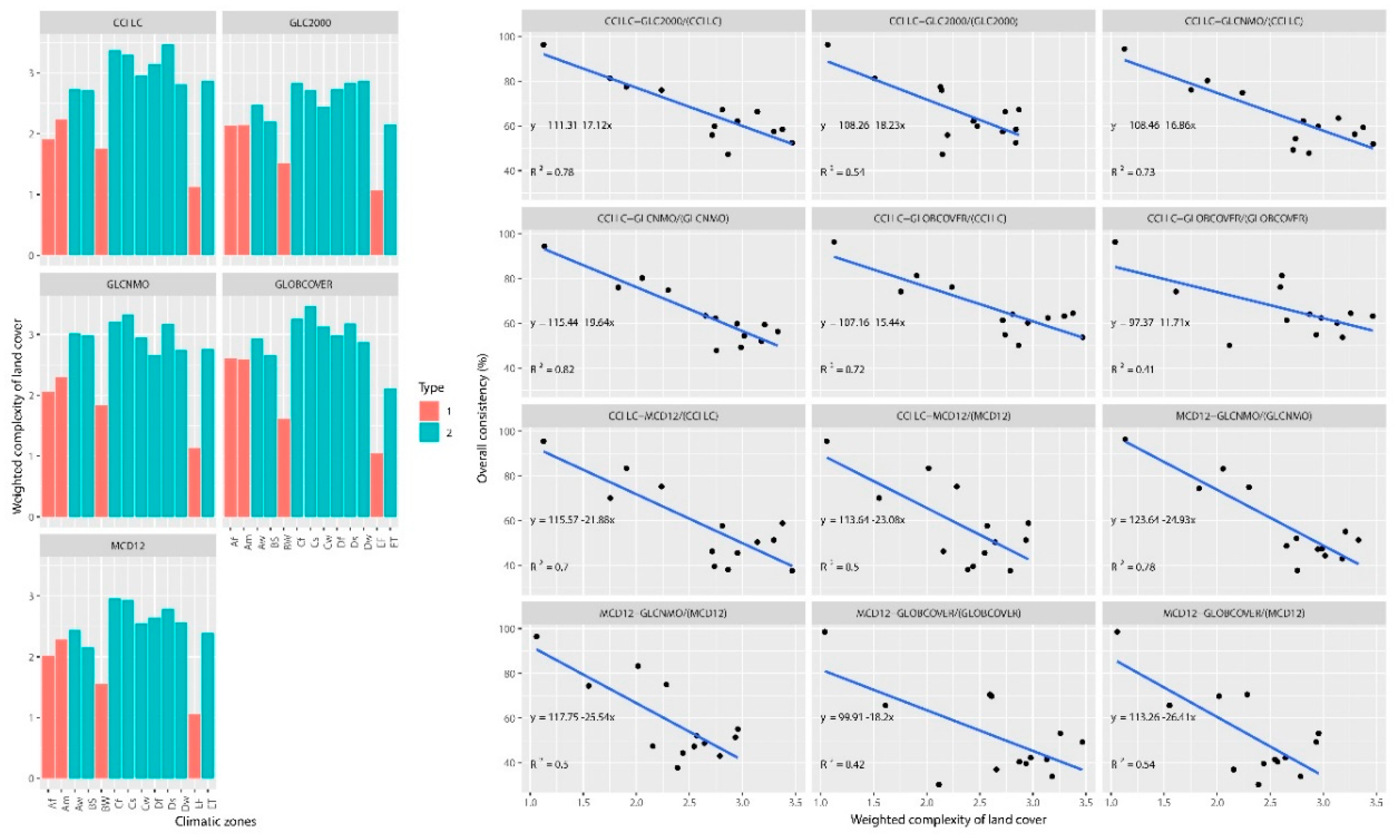
2.2.4. Weighted Complexity of the Land Cover

We call the complexity of land-cover types of a certain area as the weighted complexity of land cover. When using the focal statistics tool in ArcGIS 10.2, the number of different land-cover types within the rectangular analysis window (10 × 10 pixels) is the land-cover complexity of the central pixel of the window. We study a total of nine different land use types, so the range of the land-cover complexity is 1–9. According to the level classification of the land-cover complexity, when the land-cover complexity of a pixel is x , x different types of land cover exist within the 10 × 10 rectangular area centered on this pixel. The formula is as follows:
WCLC   = x 9 x S x x 9 S x ,
where x is the land complexity and S x is the area with land complexity x .

3. Results

3.1. Spatial Consistency at the Global and Continental Scales

3.1.1. Category Composition Similarity at the Global and Continental Scales

At the global scale, the correlation coefficients of the compositional similarity among the five datasets are quite different, ranging from 69% to 97%, and the inter-annual variation is small. Obvious intercontinental differences were observed according to the results of the intercontinental comparison (see Figure S1).

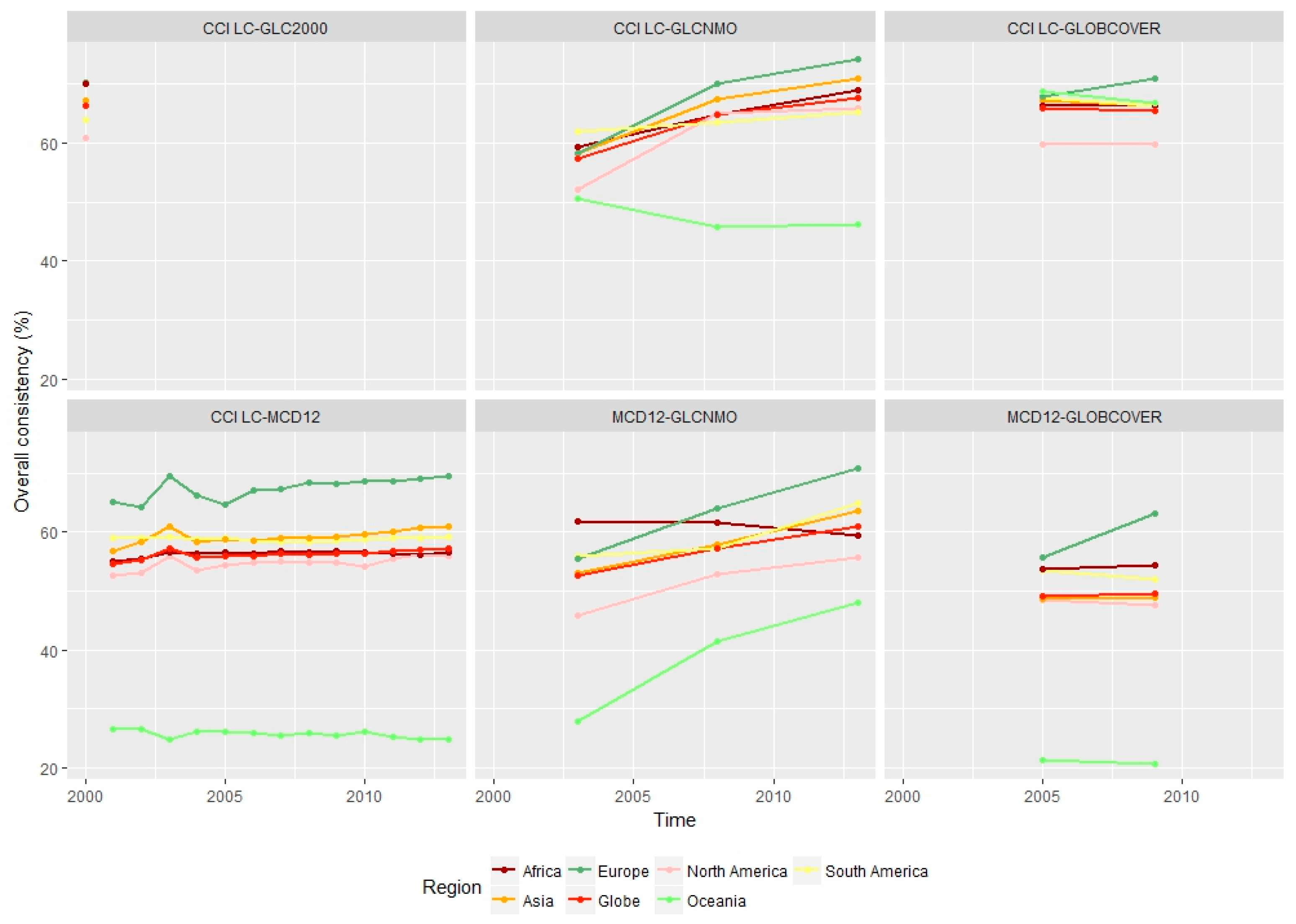
3.1.2. Overall Consistency Differences at the Global and Continental Scales

We calculate the confusion matrix of the globe and six continents to obtain the overall consistency of the datasets. Figure 1 indicates the overall inter-annual consistency of the inter-comparison of five datasets for the globe and six continents. On the global scale, the overall consistency of all the datasets is between 49.2% and 67.6%. On the continental scale, the overall consistency of some datasets presents obvious intercontinental and inter-annual differences.
As for the multi-year averages of the overall consistency on the global scale, the highest overall consistency between CCI LC and GLC2000 was 66.46%. The second highest was found between CCI LC and GLOBCOVER (65.73%). The comparison between CCI LC and GLCNMO was also relatively high (63.26%). The overall consistency between other land-cover datasets was always lower than 60%. The comparison between MCD12 and GLOBCOVER was the worst: only 49.40%. The overall global consistency of each node with GLCNMO in the comparison significantly increased with time, and the results of the comparison with CCI LC in 2013 were 10 percentage points higher than those of 2003, while the results of comparison with MCD12 in 2013 were eight percentage points higher than those of 2003.
As for the multi-year averages of the overall consistency on the continental scale, the comparison of CCI LC with GLC2000 and CCI LC with GLOBCOVER basically exceeded 60% on all continents. However, the comparison of CCI LC with GLCNMO, CCI LC with MCD12, MCD12 with GLCNMO and MCD12 with GLOBCOVER showed that the overall consistency of Oceania was much lower than that of the other continents, with multi-year averages of 47.54%, 25.71%, 39.14% and 21.04%, respectively. Meanwhile, the overall consistency of Europe was slightly higher than that of other continents in most comparisons.
In addition to the comparison in 2003 showing a sharp increase, the inter-annual variation in the overall consistency between CCI LC and MCD12 was relatively stable and the CCI LC and MCD12 multi-phase datasets likely had very stable interpretations. However, the overall consistency of the comparisons between other datasets showed varying degrees of inter-annual change. The overall consistency between MCD12 and GLOBCOVER in Europe showed significant improvement, with an increase of nearly eight percentage points. The overall consistency between CCI LC and GLCNMO and between MCD12 and GLCNMO in most regions increased each year.

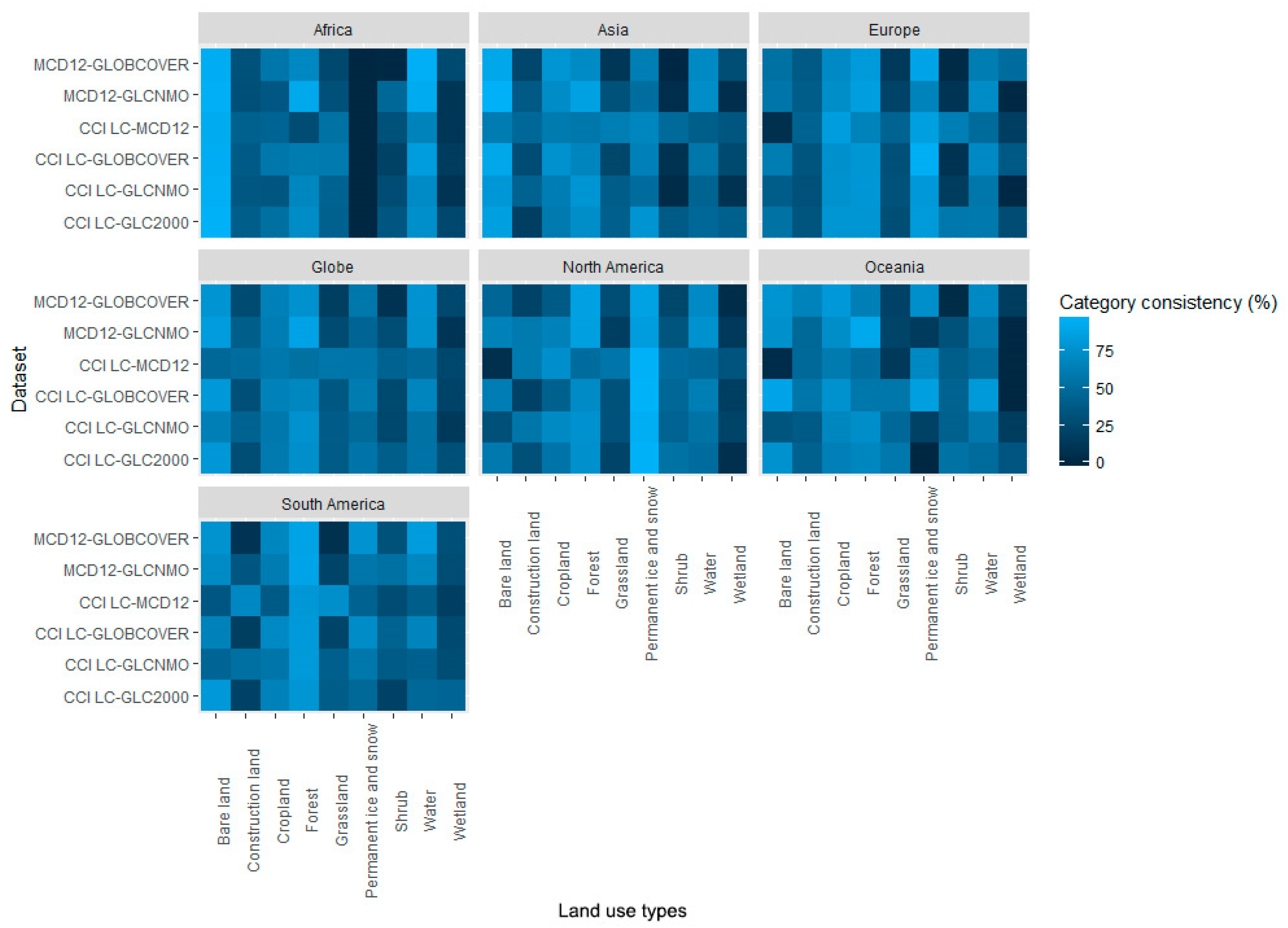
3.1.3. Category Consistency Difference at the Global and Continental Scales

These datasets spanned several years, so we calculated the multi-year average of the category consistency of each land use type. The results are shown in Figure 2.
On the global scale, the category consistency of forest and bare land was relatively high, and the average results among the datasets were 73.24% and 72.74%, respectively. The category consistency of shrub and wetland was relatively low, and the average results among the datasets were 28.48% and 20.92%, respectively. The spectral characteristics of shrubs and wetlands are not obvious, and the spatial distribution of shrubs and wetlands can easily interlace with other land objects. Therefore, the category consistency of these two land use types was lower in all the dataset comparisons.
On the continental scale, except for the comparison between MCD12 and CCI LC in Africa, the category consistency of forest in all the other datasets was higher than 60%. Forests can be easily identified because their spectral and spatial texture features are clear and easy to distinguish from other land use types, and these regions have a wide and continuous distribution on the global scale. In terms of construction land, the category consistency of each dataset was relatively low, and the degree of recognition of construction land by CCI LC and MCD12 was slightly better than for the other datasets. The identification of construction land was not high, which may have been related to the complex spectral features of construction land and the difficulty in extracting any features.
Furthermore, the category consistency of bare land in Africa and permanent ice and snow in North America was extremely high, close to or exceeding 90%, mainly because of the continuous and concentrated distribution of bare land and permanent ice and snow cover in the Sahara Desert and Greenland, respectively.

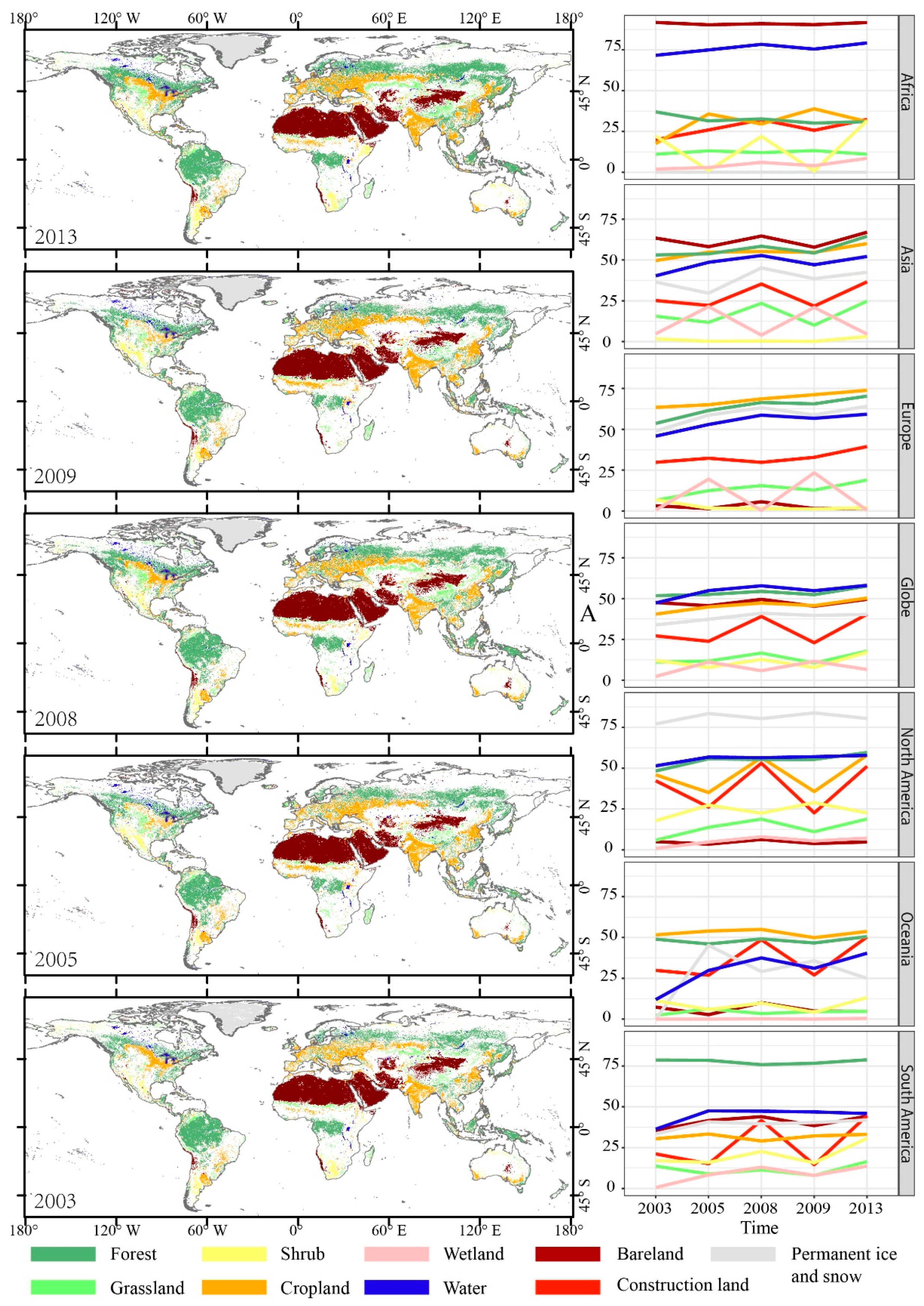
3.1.4. Spatial Multiple-Consistency at the Global and Continental Scales

Spatial multiple-consistency occurs if three datasets determine that a certain pixel is the same land use type. Three such datasets exhibited this feature for 2003, 2005, 2008, 2009 and 2013. More precisely, we used the GLCNMO, CCI LC, and MCD12 datasets to compare the spatial multiple-consistency in 2003, 2008 and 2013, while we used the GLOBCOVER, CCI LC and MCD12 datasets to calculate the spatial multiple-consistency in 2005 and 2009. Figure 3 illustrates the spatial multiple- consistency of nine land use types on six continents and across the globe and describes the characteristics of the spatial distribution of these land use types.
The spatial multiple-consistency of forest was high in South America, Europe, and Asia, higher than 75%, 50%, and 50%, respectively, including being widely distributed in the Amazon Plain, western Pampas, Southeast Asia, Korean Peninsula, and the middle and lower reaches of the Yangtze River in Asia. The spatial multiple-consistency of cropland was high in Europe, Asia, and Oceania, with values higher than 57.5%, 50%, and 50%, respectively. The spatial multiple-consistency of construction land was low across all six continents: less than 50%. At the same time, the spatial multiple-consistency of grassland, wetland, shrub was also low on all six continents, with values less than 25%.
The spatial multiple-consistency of bare land widely varied across all continents, with a high consistency of more than 90% in Africa, while the spatial multiple-consistency in Europe, Oceania, and North America was close to 0. Bare land was mainly concentrated in the Sahara Desert, Arabian Peninsula, Iranian Plateau, Taklamakan Desert, and Mongolian Plateau. The spatial multiple- consistency of water on each continent except Africa and Oceania was approximately 50%. The distribution of water was basically the same as the world’s important water lakes and rivers. Permanent ice and snow was highly spatially consistent in North America, and the values of the five time nodes were more than 75%, while permanent ice and snow was mainly distributed in the high latitudes of the Northern Hemisphere, such as in Greenland and Svalbard. However, water and forests had high spatial consistency on the global scale, often exceeding 50%, and grassland, shrub and wetland were less than 20%. Generally, a large number of inconsistent areas were present in central and southern Africa, northern high latitudes outside Greenland, and most of Australia. Subsequent global land-cover datasets should focus on the above areas.

3.2. Spatial Consistency of Elevation and Climatic Zones

3.2.1. Overall Consistency Differences of Continental Elevations

The overall consistency of continental elevation greatly fluctuated with variations in elevation, but the fluctuation trend of each dataset was close. Twenty-four elevation gradient intervals were observed across the six continents. Six datasets exhibited consistent characteristics in two thirds of the intervals. However, at least five datasets had consistent features in 22 intervals, or 91.67% of the total (see Figure S2).

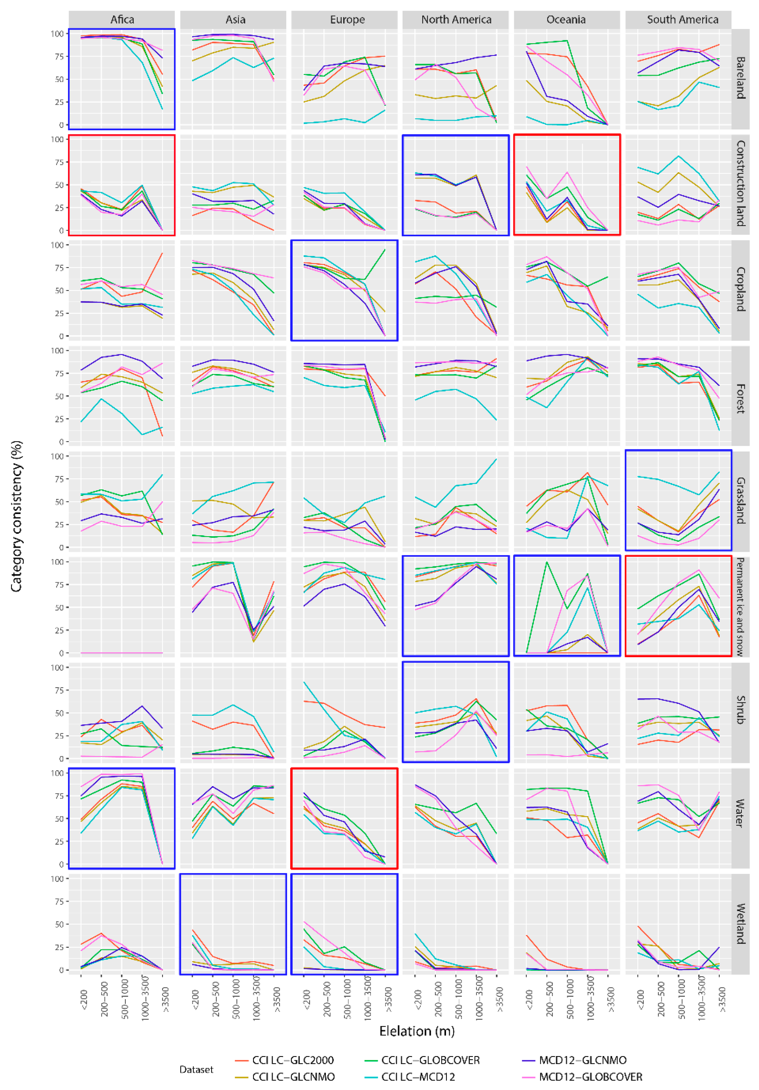
3.2.2. Category Consistency Differences of Continental Elevations

Figure 4 illustrates the gradient characteristics of the category consistency with elevation changes for the nine land use types on all six continents. The results show that the datasets had relatively poor consistency in the description of category consistency of the elevation gradient features: four comparison results showed that six datasets consistently characterized the gradient features, and 10 comparison features showed that five datasets presented similar gradient features. That is to say, the comparison results of at least five datasets appeared to be consistent in only one quarter.
Africa had three types of land-type gradients with similar characteristics. For Asia, the spatial consistency gradients of wetland were similar, and the spatial consistency of water and permanent ice and snow showed an obvious fluctuation with increasing elevation. The gradient characteristics of the spatial consistency of cropland, water and wetland in Europe were similar. In Oceania, the consistency gradients of construction land and permanent ice and snow were similar, and the characteristics of the consistency gradients of grassland and permanent ice and snow in South America were similar. More than 75% of the results showed that the consistency above 3500 m was lower than that for 1000–3500 m, whose value was 57.40%, while the values of the other two intervals were 54.31% and 43.21% for all six continents.

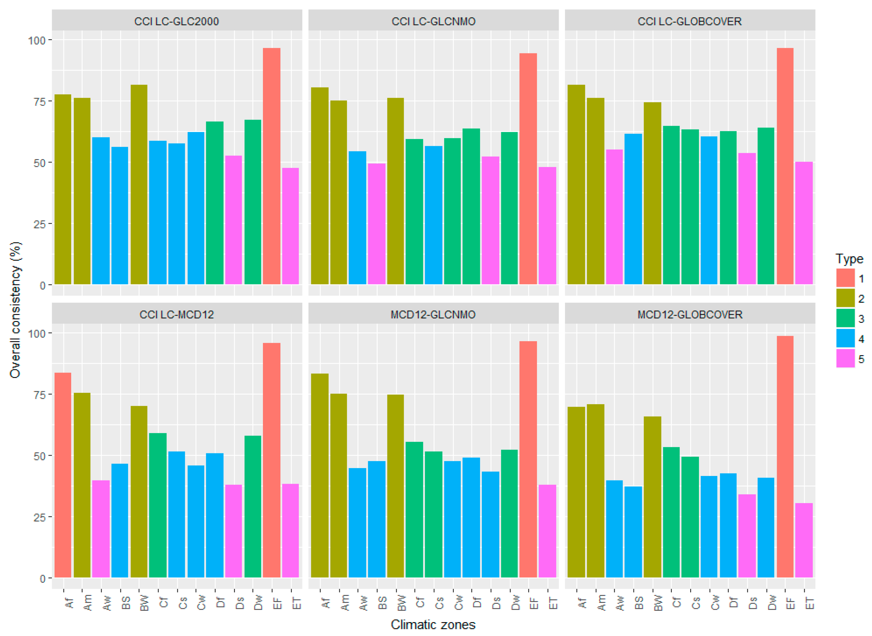
3.2.3. Overall Consistency Differences of Climatic Zones

Figure 5 shows the overall consistency of the comparison results among the various climate sub-regions, which were divided into five categories based on the natural-breaks method.
The six comparison results exhibited consistency in the first, second and fifth categories. The overall consistency of the EF region was significantly higher than that of other regions: close to 95%. The overall consistency of Af, Am and Bw was also relatively high, with averages of 79.21%, 74.63% and 73.60%, respectively. Meanwhile, the six comparison results showed that the overall consistency in Ds and ET was relatively poor, with averages of 45.44% and 41.92%, respectively. However, the overall consistency of the other climatic zones in the six comparison results greatly fluctuated.
We calculated the standard deviation of the spatial consistency of each climatic zone to quantify the differences in the overall consistency of each climate zone. The average standard deviation of the six comparisons was 15.33, and a certain degree of spatial-consistency difference was observed in the climatic zone. At the same time, except for the results of CCI LC compared to MCD12, the standard deviation of the results of the MCD12 participation comparison had an average value of 17.98, which was significantly higher than that of CCI LC, whose average was 12.81. In short, large differences were present in the overall consistency of each climatic zone. According to the comparison results, the overall consistency of the EF, Af, Am and Bw climatic zones was higher, while that of the Ds and ET climatic zones was lower.

3.2.4. Category Consistency Differences of Climatic Zones

Factors such as the temperature and precipitation created large differences in the land use types’ composition in each climatic zone, which affected the category consistency (see Figure S3).

4. Discussion

4.1. Advantages of Temporal Consistency and Geographical Zoning on Spatial Assessment

According to the above comparison and analyses, the spatial consistency among these datasets was not high. This finding is not surprising and matches earlier conclusions by DeFries, Hansen and Latifovic [50,51,52]. This finding could either be real or simply be caused by differences in sensors, temporal periods, original classification algorithms, or classification schemes [53]. In addition, we have some thoughts on the role of maintaining temporal consistency and basing the analysis on geographical zoning research to consistently compare datasets.
First, maintaining temporal consistency is useful to reduce the effect of land-cover changes on the comparison. Scholars found that land-cover changes between the acquisition datasets can affect such comparisons [29,54], and the purpose of maintaining temporal consistency is to abandon the original cross-time comparison and reduce the effect of land-cover changes on the comparison. According to previous research, some land use types, such as water and cropland, have greatly changed on the global and continental scales, and values on smaller scales may hide heterogeneities among regions [55,56]. In other words, land-cover changes in local areas are dramatic and may not be the primary factor but are still critical in comparisons.
Second, we can observe whether the interpretation ability of the same set of datasets varies between years by maintaining temporal consistency. According to the comparison between GLOBCOVER and CCI LC, GLOBCOVER and MCD12 in Figure 1, the consistency of the European region was greatly improved and the comparison between CCI LC and MCD12 in 2003 significantly deviated compared to other years. In other words, the interpretation of multiphase datasets may be less stable, and the interpretation consistency of a certain area at a certain time node for a set of land datasets does not present interpretation consistency for all the datasets.
Third, we chose to compare the spatial consistency in geography-based schemes, such as elevation and climatic zones, rather than administrative areas (continental or national scales). Compared to administrative areas, the composition of geography-based schemes is more regular, and we could find features of consistency in homogeneous or heterogeneous environments. The consistency of many datasets above 3500 m declined somewhat compared to the consistency at elevations between 1000 and 3500 m. The consistency of different climate zones was also somewhat different, suggesting that the input data source, classification scheme, and classification methodology were all optimized to the features of regional heterogeneity.

4.2. Inconsistencies from Surface Conditions

Temperature and precipitation factors affect the surface composition of the Earth’s surface. Compared to continents, the composition of surface conditions in different climatic zones can be more regular, which could result in inconsistencies in land-cover datasets. It is noted that this study used the method of weighted complexity of land cover to measure the land pattern in each climatic zone. It contributes to explore the relationship between spatial consistency and the weighted complexity of land cover.
Figure 6 shows the weighted complexity of the land cover in each climatic zone and regression equations between the overall consistency and weighted complexity of land cover in different climatic zones. Based on the results, the weighted complexity of the land cover in climatic zones with relatively high overall consistency is relatively low. As the weighted complexity of the land cover increases, the overall consistency significantly linearly declines.
In the EF, the average monthly temperature of the hottest months was below 0 °C, and snow remained accumulated throughout the year, resulting in large snow-covered areas (around 95% of the area). The spectral characteristics of snow and ice are also very clear and easy to distinguish from other features, so the overall consistency is very high: around 95%. The average overall consistency of Am was 79.21%, and Af is hot and rainy throughout the year, with an average monthly rainfall of more than 60 mm, resulting in the growth of forests and widespread distribution. Forests’ spectral and spatial texture features are clear and easy to distinguish from those of other types. Except for the small amount of mixed forest and cropland in the area, fewer mixed types were present, so the overall consistency was higher. The average overall consistency of Am was 74.63%, with the dry months during winter. The monthly precipitation may have been less than 60 mm, but the overall rainfall was sufficient. Trees grew densely and had high distribution. Except for a small amount of forest that was mixed with cropland, mixed areas were also relatively scarce and the overall consistency was higher. The average overall consistency of Bw was 73.60%. Little rain falls throughout the year, and this region contains areas where bare land is highly concentrated, such as the Sahara Desert and Arabian Plateau. Bare land occupies around 70% of the area, so the overall consistency was relatively higher. In summary, the surface conditions caused inconsistencies to some extent. The more complex the surface was, the greater the inconsistency became.

4.3. Inconsistencies from Dataset Producers

The dataset-development rules that have been established by dataset producers, including the classification schemes, classification method, connotation of land use types, resolution size, and selected time nodes of images and international participation may also result in inconsistencies among land-cover datasets.
Differences in the classification schemes and subordinate definitions of land use types among datasets are one of the major factors that create deviations in classification results, and classification schemes also make the rigorous comparison and synergistic use of different maps challenging, if not impossible [25,54,57,58]. The five datasets that were used in this study are based on two land-classification systems: LCCS and IGBP. Each land-use dataset has different definitions for their land-use types. For example, shrub forests are divided into evergreen shrubs and deciduous shrubs in GLC2000 and CCI LC; however, both are merged into shrubs in GLOBCOVER 2005/2009. Forests and other natural vegetation mosaics are subdivided into forest/shrub/grass mosaics in GLC2000 and grassland/woodland/shrub mosaics in GLOBCOVER 2005/2009 and CCI LC. The classification scheme of a dataset can affect the consistency of datasets, and the definition of land use types based on these classification schemes can create differences in interpretations from remote-sensing classification. For example, MCD12’s height threshold for dividing forests and shrubs is 2 m, while that in GLOBCOVER is 5 m and that in GLC2000 is 3 m. Therefore, the classification principles of these datasets require further investigation, and the connotation of land use types requires further revision to reduce the uncertainty in these classification schemes’ development.
In addition, maps with more detailed classes are often transformed into generalized schemes with fewer classes in dataset comparison, which naturally removes the ability to describe detailed LC characteristics [59].
Three of the five types of datasets were based on artificially assisted supervised classification. The subjectivity of visual interpretation directly affects the accuracy of translation. The GLCNMO and MCD12 datasets use the decision tree method for mapping. However, the process of setting cell values in the leaf nodes of the decision tree causes the dominant categories to be overestimated and the non-dominant categories to be underestimated.
The area, spectral information and other features of many land use types fluctuate because of seasonal changes, and images that are captured by the issuing agency of the land-cover dataset may not be consistent between months. If the selected image was taken in the dry season, the water-identification capacity will be reduced. Using image data during the non-growing season of vegetation will also reduce the interpretation results of vegetation types.
The spatial resolution of datasets that are issued by institutions is different. Higher spatial resolution can effectively describe land-cover features, especially complex surface conditions. For example, the spatial resolution of GLCNMO in 2003 was 1 km, increasing to 500 m in 2008 and 2013, and the spatial consistency was significantly improved. Many classification principles of vegetation are based on these criteria and are defined from an ecological perspective, such as tree height and canopy density, which were difficult thresholds to be detected by the coarse-resolution images that were used in these mapping projects [58].
More than 30 countries and regional and international organizations participated in the development of GLC2000. The input data source, classification scheme, and classification methodology were all optimized to the needs of the participating institutions based on the land-cover types in their respective regions [27]. Because of this overwhelming participation, the overall consistency of the CCI LC from GLC2000 was relatively small according to Figure 1.

4.4. Lessons of Global Land-Cover Mapping

According to the previous analysis, results of globe, continent, and local area all have large inconsistencies, and the complexity of land and the processing of datasets by issuing agencies can greatly affect the inconsistency of datasets (specifications of spatial consistency on some regional land cover datasets are shown in Figure S4). We should also realize that land-cover mapping is a long-term process. To meet the needs of dataset construction, we hereby propose the following suggestions.
First, subsequent classification research should focus on areas with high land-cover complexity to further improve the classification accuracy. The problem of forest-grass-shrub mixing because of their similar spectra could be solved by combining topographical features and regional vegetation phenotypic data to reduce errors.
Second, the data producer should disclose the completed and detailed mapping process and dataset features, including the time information of each view of the dataset, which is convenient for the user to optimize and reclassify the dataset locally according to the characteristics of the time distribution and the research needs.
Third, radar data are sensitive to underlying water in vegetation; backscattered signals significantly increase when the ground floor is covered by water [60,61,62]. Dataset publications should consider using radar data to participate in the classification of land use types and improve the interpretation accuracy of wetland. Furthermore, cloud cover may cause problems in large areas of the humid tropics during a considerable portion of the year [63]. Radar images may overcome these problems to some extent [64,65].
Fourth, construction land classification on the global scale faces enormous challenges because of the small patch size. Several studies showed that the imagery of nighttime lights can effectively extract construction-land areas [66,67,68], and the feasibility of these data should increase with the launch of the 130 m resolution LJ01 nighttime-lighting satellite. In global land mapping, we can consider the integration of nighttime-lighting data to improve the classification accuracy of construction land.
Finally, significant regional differences in spatial consistency exist among land-cover datasets based on previous research. Datasets that are developed by regional or national cooperation must ensure that the quality of datasets is consistent at the global scale.

5. Conclusions

Based on the premise of temporal consistency, this paper compared the spatial consistency of five datasets, including GLC2000, CCI LC, MCD12, GLOBCOVER, and GLCNMO, from 2000 to 2013 at the global and continent scales. This research was conducted through composition similarity analysis, confusion matrix analysis, and spatial multiple-consistency analysis and examined inter-annual changes. At the same time, we studied the gradient characteristics of the spatial consistency of five datasets at different elevations and climatic zones. From the two angles of the surface conditions and dataset producers, the influence factors of the spatial consistency were determined and suggestions for global land-cover mapping were proposed. The conclusions are summarized as follows.
At the global scale, the average compositional similarity among five datasets was 70.82%, and the inter-annual variation was small. The mean overall consistency of all the datasets was 56.58%, and much room for improvement was observed. The spatial consistency of cropland, forests, water, bare land, and permanent ice and snow was close to or higher than 50%, while the spatial consistency of wetland and shrub was less than 50%. At the continental scale, the results of multiple datasets showed obvious intercontinental differences in the compositional similarity and overall consistency: Europe’s composition similarity and overall consistency was higher, while those of Oceania were extremely low. The trend depiction of each dataset was more consistent in the elevation gradient of the overall consistency, especially in North America and Asia, and the comparison of the six datasets was completely consistent. For the spatial consistency of the climate-zone gradient, the results of the dataset comparison showed that the overall consistency of the EF, Af, Am and BW regions was higher, while the overall consistency of ET and Ds was the worst. The classification schemes, classification method, connotation of land use types, resolution size, selected time nodes for images and international participation, and the complex situation of surface conditions can greatly influence the spatial consistency.
This study showed that the spatial consistency of global datasets is characterized by spatial heterogeneity, that is, the consistency of different regions is quite different. Although the development of these land-cover datasets greatly promotes scientific research, satisfying the needs of high-precision land-surface-process simulations remains difficult. For the future development of global land-cover datasets, more attention should be paid to the experiences of previous global land-cover mapping activities, including land-cover classification in complex areas and regional representative classification sample selection.
In addition, it would be more effective if some validation points were used in case the lack of some validation points will lead to some uncertainty about the results of our research. While it is difficult for us to collect validation points from multiple time periods on a global scale, we believe that there is also a certain confidence through cross comparison between datasets. In addition, our work will be more useful if consulting with the advanced measures of thematic classification accuracy. Furthermore, our research only focused on medium resolution land-cover datasets and did not adopt GlobeLand30, for it has a resolution of 30 meters, which is significantly higher than other datasets we used. If there are more 30-meter resolution global land cover datasets in the future, we will compare the spatial consistency of these datasets including GlobeLand30.

Supplementary Materials

The following are available online at https://www.mdpi.com/2072-4292/10/11/1846/s1.

Author Contributions

W.Z. and Y.L. conceived and designed the research. T.H. conducted the analysis and drafted the manuscript. S.W. and S.Y. provided some essential suggestions regarding the consistency assessment. All the authors contributed to the discussion of the results and edited the manuscript.

Funding

This research was funded by the National Key R&D program of China, grant number 2017YFA0604704, National Natural Science Foundation of China, grant number 41771197 and State Key Laboratory of Earth Surface Processes and Resource Ecology, grant number2017-FX-01(2).

Acknowledgments

The authors thank four anonymous referees for their constructive comments on this paper and are indebted to the individuals who have contributed to the generation of the five global land cover data sets compared in this study.

Conflicts of Interest

The authors declare no conflicts of interest.

References

  1. Foley, J.A.; Defries, R.; Asner, G.P.; Barford, C.; Bonan, G.; Carpenter, S.R.; Chapin, F.S.; Coe, M.T.; Daily, G.C.; Gibbs, H.K. Global consequences of land use. Science 2005, 309, 570–574. [Google Scholar] [CrossRef] [PubMed]
  2. Turner, B.L.; Lambin, E.F.; Reenberg, A. The emergence of land change science for global environmental change and sustainability. Proc. Natl. Acad. Sci. USA 2007, 104, 20666–20671. [Google Scholar] [CrossRef] [PubMed] [Green Version]
  3. Bonan, G.B. The land surface climatology of the NCAR land surface model coupled to the NCAR community climate model*. J. Clim. 2002, 15, 3123–3149. [Google Scholar] [CrossRef]
  4. Running, S.W.; Nemani, R.R.; Heinsch, F.A.; Zhao, M.; Reeves, M.; Hashimoto, H. A continuous satellite-derived measure of global terrestrial primary production. Bioscience 2004, 54, 547–560. [Google Scholar] [CrossRef]
  5. Zhang, K.; Kimball, J.S.; Mu, Q.; Jones, L.A.; Goetz, S.J.; Running, S.W. Satellite based analysis of northern et trends and associated changes in the regional water balance from 1983 to 2005. J. Hydrol. 2009, 379, 92–110. [Google Scholar] [CrossRef]
  6. Stehman, S. Basic probability sampling designs for thematic map accuracy assessment. Int. J. Remote Sens. 1999, 20, 2423–2441. [Google Scholar] [CrossRef]
  7. Mcroberts, R.E. Probability- and model-based approaches to inference for proportion forest using satellite imagery as ancillary data. Remote Sens. Environ. 2010, 114, 1017–1025. [Google Scholar] [CrossRef]
  8. Sutherland, W.J.; Adams, W.M.; Aronson, R.B.; Aveling, R.; Blackburn, T.M.; Broad, S.; Ceballos, G.; Côté, I.M.; Cowling, R.M.; Fonseca, G.A.B.D. One hundred questions of importance to the conservation of global biological diversity. Conserv. Boil. 2009, 23, 557–567. [Google Scholar] [CrossRef] [PubMed]
  9. Chen, B.; Chen, J.M.; Ju, W. Remote sensing-based ecosystem–atmosphere simulation scheme (EASS)—model formulation and test with multiple-year data. Ecol. Model. 2007, 209, 277–300. [Google Scholar] [CrossRef]
  10. Sellers, P.J.; Randall, D.A.; Collatz, G.J.; Berry, J.A.; Field, C.B.; Dazlich, D.A.; Zhang, C.; Collelo, G.D.; Bounoua, L. A Revised Land Surface Parameterization (SiB2) for Atmospheric GCMs. Part I: Model Formulation. J. Clim. 1996, 9, 676–705. [Google Scholar] [CrossRef]
  11. Dai, Y.; Zeng, X.; Dickinson, R.E.; Baker, I.; Bonan, G.B.; Bosilovich, M.G.; Denning, A.S.; Dirmeyer, P.A.; Houser, P.R.; Niu, G. The common land model. Bull. Am. Meteor. Soc. 2015, 1, 1013–1023. [Google Scholar] [CrossRef]
  12. Yu, L.; Su, J.; Li, C.; Wang, L.; Luo, Z.; Yan, B. Improvement of moderate resolution land use and land cover classification by introducing adjacent region features. Remote Sens. 2018, 10, 414. [Google Scholar] [CrossRef]
  13. Matthews, E. Global vegetation and land use: New high-resolution data bases for climate studies. J. Clim. Appl. Meteorol 1983, 22, 474–487. [Google Scholar] [CrossRef]
  14. Olson, J.S.; Watts, J.S. Major World Ecosystem Complexes; Oak Ridge National Laboratory: Oak Ridge, TN, USA, 1982.
  15. Henderson-Sellers, A.; Wilson, M.F.; Thomas, G.; Dickinson, R.E. Current Global Land-Surface Data Sets for Use in Climate Related Studies; NCAR: Boulder, CO, USA, 1985. [Google Scholar]
  16. Defries, R.; Hansen, M.; Townshend, J. Global discrimination of land cover types from metrices derived from AVHRR pathfinder data. Remote Sens. Environ. 1995, 54, 209–222. [Google Scholar] [CrossRef]
  17. Loveland, T.R.; Belward, A.S. The IGBP-DIS global 1 km land cover data set, discover: First results. Int. J. Remote Sens. 1997, 18, 3289–3295. [Google Scholar] [CrossRef]
  18. Loveland, T.R.; Reed, B.C.; Brown, J.F.; Ohlen, D.O.; Zhu, Z.; Yang, L.; Merchant, J.W.; Defries, R.S.; Belward, A.S. Development of a global land cover characteristics database and IGBP discover from 1 km AVHRR data. Int. J. Remote Sens. 2000, 21, 1303–1330. [Google Scholar] [CrossRef]
  19. Arino, O.; Bicheron, P.; Achard, F.; Latham, J.; Witt, R.; Weber, J.L. Globcover: The most detailed portrait of earth. ESA Bull. Bull. ASE. Eur. Space Agency 2008, 2008, 24–31. [Google Scholar]
  20. Bicheron, P.; Defourny, P.; Brockmann, C.; Schouten, L.; Vancutsem, C.; Huc, M.; Bontemps, S.; Leroy, M.; Achard, F.; Herold, M. Globcover: Products description and validation report. Foro Mund. De La Salud 2011, 17, 285–287. [Google Scholar]
  21. Defourny, P.; Kirches, G.; Brockmann, C.; Boettcher, M.; Peters, M.; Bontemps, S.; Lamarche, C.; Schlerf, M.; Santoro, M. Land Cover CCI: Product User Guide Version 2. Available online: http://maps.elie.ucl.ac.be/CCI/viewer/download/ESACCI-LC-PUG-V2.4.pdf (accessed on 11 June 2015).
  22. Brown, J.F.; Loveland, T.R.; Ohlen, D.O. The global land-cover characteristics database: The users’ perspective. Photogramm. Eng. Remote Sens. 1999, 65, 1069–1074. [Google Scholar]
  23. Foody, G.M. Status of land cover classification accuracy assessment. Remote Sens. Environ. 2002, 80, 185–201. [Google Scholar] [CrossRef]
  24. Foody, G.M. Assessing the accuracy of land cover change with imperfect ground reference data. Remote Sens. Environ. 2010, 114, 2271–2285. [Google Scholar] [CrossRef] [Green Version]
  25. Herold, M.; Mayaux, P.; Woodcock, C.E.; Baccini, A.; Schmullius, C. Some challenges in global land cover mapping: An assessment of agreement and accuracy in existing 1km datasets. Remote Sens. Environ. 2008, 112, 2538–2556. [Google Scholar] [CrossRef]
  26. Fritz, S.; See, L.; Rembold, F. Comparison of global and regional land cover maps with statistical information for the agricultural domain in Africa. Int. J. Remote Sens. 2010, 31, 2237–2256. [Google Scholar] [CrossRef]
  27. Giri, C.; Zhu, Z.; Reed, B. A comparative analysis of the global land cover 2000 and MODIS land cover data sets. Remote Sens. Environ. 2005, 94, 123–132. [Google Scholar] [CrossRef]
  28. Mccallum, I.; Obersteiner, M.; Nilsson, S.; Shvidenko, A. A spatial comparison of four satellite derived 1 km global land cover datasets. Int. J. Appl. Earth Obs. Geoinf. 2006, 8, 246–255. [Google Scholar] [CrossRef]
  29. Tchuenté, A.T.K.; Roujean, J.L.; Jong, S.M.D. Comparison and relative quality assessment of the GLC2000, GLOBCOVER, MODIS and ECOCLIMAP land cover data sets at the African continental scale. Int. J. Appl. Earth Obs. Geoinf. 2011, 13, 207–219. [Google Scholar] [CrossRef]
  30. Latifovic, R.; Olthof, I. Accuracy assessment using sub-pixel fractional error matrices of global land cover products derived from satellite data. Remote Sens. Environ. 2004, 90, 153–165. [Google Scholar] [CrossRef]
  31. Ran, Y.; Li, X.; Lu, L. Evaluation of four remote sensing based land cover products over China. Int. J. Remote Sens. 2010, 31, 391–401. [Google Scholar] [CrossRef]
  32. Wu, W.; Shibasaki, R.; Ongaro, L.; Ongaro, L.; Zhou, Q.; Tang, H. Validation and comparison of 1 km global land cover products in China. Int. J. Remote Sens. 2008, 29, 3769–3785. [Google Scholar] [CrossRef]
  33. Song, X.P.; Hansen, M.C.; Stehman, S.V.; Potapov, P.V.; Tyukavina, A.; Vermote, E.F.; Townshend, J.R. Global land change from 1982 to 2016. Nature 2018, 560, 639–643. [Google Scholar] [CrossRef] [PubMed]
  34. Seto, K.C.; Michail, F.; Burak, G.; Reilly, M.K. A meta-analysis of global urban land expansion. PLoS ONE 2011, 6, e23777. [Google Scholar] [CrossRef] [PubMed]
  35. Dewan, A.M.; Yamaguchi, Y. Land use and land cover change in Greater Dhaka, Bangladesh: Using remote sensing to promote sustainable urbanization. Appl. Geogr. 2009, 29, 390–401. [Google Scholar] [CrossRef]
  36. Bartholome, E.; Belward, A.S. Glc2000: A new approach to global land cover mapping from earth observation data. Int. J. Remote Sens. 2005, 26, 1959–1977. [Google Scholar] [CrossRef]
  37. Friedl, M.A.; Sulla-Menashe, D.; Tan, B.; Schneider, A.; Ramankutty, N.; Sibley, A.; Huang, X. Modis collection 5 global land cover: Algorithm refinements and characterization of new datasets. Remote Sens. Environ. 2010, 114, 168–182. [Google Scholar] [CrossRef]
  38. Kasimu, A. Production of global land cover data—GLCNMO. J. Geogr. Geol. 2011, 4, 22–49. [Google Scholar]
  39. European Space Agency Climate Change Initiative. Available online: http://maps.elie.ucl.ac.be/CCI/viewer/index.php (accessed on 21 November 2018).
  40. The Global Land Cover by National Mapping Organizations. Available online: https://globalmaps.github.io/glcnmo.html (accessed on 21 November 2018).
  41. European Space Agency GlobCover Portal. Available online: http://due.esrin.esa.int/page_globcover.php (accessed on 21 November 2018).
  42. USGS Earth Resources Observation and Science (EROS) Center. Available online: https://e4ftl01.cr.usgs.gov/MOTA/ (accessed on 21 November 2018).
  43. Joint Research Centre, the European Commission’s Science and Knowledge Service. Available online: http://forobs.jrc.ec.europa.eu/products/glc2000/products.php (accessed on 21 November 2018).
  44. World Maps of KOPPEN-GEIGER Climate Classification. Available online: http://koeppen-geiger.vu-ien.ac.at/ (accessed on 21 November 2018).
  45. Hu, Y.; Zhang, Q.; Dai, Z.; Huang, M.; Yan, H. Agreement analysis of multi-sensor satellite remote sensing derived land cover products in the Europe Continent. Geogr. Res. 2015, 34, 1839–1852. (In Chinese) [Google Scholar]
  46. Canters, F. Evaluating the uncertainty of area estimates derived from fuzzy land-cover classification. Photogramm. Eng. Remote Sens. 1997, 63, 403–414. [Google Scholar]
  47. Liu, F.; Chinitz, L.M.; Abe, K.; Breedon, R.E.; Fujii, Y.; Kurihara, Y.; Maki, A.; Nozaki, T.; Omori, T.; Sagawa, H. A scalable approach to mapping annual land cover at 250 m using MODIS time series data: A case study in the Dry Chaco ecoregion of South America. Remote Sens. Environ. 2010, 114, 2816–2832. [Google Scholar]
  48. Fung, T.; Ledrew, E.F. The determination of optimal threshold levels for change detection using various accuracy indices. Photogramm. Eng. Remote Sens. 1988, 54, 1449–1454. [Google Scholar]
  49. Janssen, L.L.F.; Wel, F.J.M.V.D. Accuracy assessment of satellite derived land cover data: A review. Photogramm. Eng. Remote Sens. 1994, 60, 419–426. [Google Scholar]
  50. Defries, R.; Townshend, J. Ndvi-derived land cover classification at global scales. Int. J. Remote Sens. 1994, 15, 3567–3586. [Google Scholar] [CrossRef]
  51. Hansen, M.C.; Reed, B.; Defries, R.S.; Belward, A.S. A comparison of the igbp discover and university of maryland 1 km global land cover products. Int. J. Remote Sens. 2000, 21, 1365–1373. [Google Scholar] [CrossRef]
  52. Latifovic, R.; Zhu, Z.L.; Cihlar, J.; Giri, C.; Olthof, I. Land cover mapping of north and central America—global land cover 2000. Remote Sens. Environ. 2004, 89, 116–127. [Google Scholar] [CrossRef]
  53. Bai, Y.; Feng, M.; Jiang, H.; Wang, J.; Zhu, Y.; Liu, Y. Assessing consistency of five global land cover data sets in China. Remote Sens. 2014, 6, 8739–8759. [Google Scholar] [CrossRef]
  54. Jung, M.; Henkel, K.; Herold, M.; Churkina, G. Exploiting synergies of global land cover products for carbon cycle modeling. Remote Sens. Environ. 2006, 101, 534–553. [Google Scholar] [CrossRef]
  55. Pérezhoyos, A.; Rembold, F.; Kerdiles, H.; Gallego, J. Comparison of global land cover datasets for cropland monitoring. Remote Sens. 2017, 9. [Google Scholar] [CrossRef]
  56. Allen, G.H.; Pavelsky, T.M. Global extent of rivers and streams. Science 2018, 361, 585–588. [Google Scholar] [CrossRef] [PubMed]
  57. Gong, P.; Wang, J.; Yu, L.; Zhao, Y.; Zhao, Y.; Liang, L.; Niu, Z.; Huang, X.; Fu, H.; Liu, S. Finer resolution observation and monitoring of global land cover: First mapping results with Landsat tm and ETM+ data. Int. J. Remote Sens. 2013, 34, 2607–2654. [Google Scholar] [CrossRef]
  58. Congalton, R.G.; Gu, J.; Yadav, K.; Thenkabail, P.; Ozdogan, M. Global land cover mapping: A review and uncertainty analysis. Remote Sens. 2014, 6, 12070–12093. [Google Scholar] [CrossRef]
  59. Yang, Y.; Xiao, P.; Feng, X.; Li, H. Accuracy assessment of seven global land cover datasets over China. ISPRS J. Photogramm. Remote Sens. 2017, 125, 156–173. [Google Scholar] [CrossRef]
  60. Eric, S.K. Moritoring south Florida wetlands using ERS-1 SAR imagery. Photogramm. Eng. Remote Sens. 1997, 63, 281–291. [Google Scholar]
  61. Martinez, J.M.; Toan, T.L. Mapping of flood dynamics and spatial distribution of vegetation in the amazon floodplain using multitemporal SAR data. Remote Sens. Environ. 2007, 108, 209–223. [Google Scholar] [CrossRef]
  62. Baghdadi, N.; Bernier, M.; Gauthier, R.; Neeson, I. Evaluation of c-band SAR data for wetlands mapping. Int. J. Remote Sens. 2001, 22, 71–88. [Google Scholar] [CrossRef]
  63. Ju, J.; Roy, D.P. The availability of cloud-free Landsat ETM+ data over the conterminous United States and globally. Remote Sens. Environ. 2008, 112, 1196–1211. [Google Scholar] [CrossRef]
  64. Defries, R. Terrestrial vegetation in the coupled human-earth system: Contributions of remote sensing. Soc. Sci. Electron. Publ. 2008, 33, 369–390. [Google Scholar] [CrossRef]
  65. Freitas, C.D.C.; Soler, L.D.S.; Sant’Anna, S.J.S.; Dutra, L.V.; Santos, J.R.D.; Mura, J.C.; Correia, A.H. Land use and land cover mapping in the brazilian amazon using polarimetric airborne p-band SAR data. IEEE Trans. Geosci. Remote Sens. 2008, 46, 2956–2970. [Google Scholar] [CrossRef]
  66. Schneider, A. A new map of global urban extent from MODIS satellite data. Environ. Res. Lett. 2009, 4, 44003–44011. [Google Scholar] [CrossRef]
  67. Liu, Z.; He, C.; Zhang, Q.; Huang, Q.; Yang, Y. Extracting the dynamics of urban expansion in China using DMSP-OLS nighttime light data from 1992 to 2008. Landsc. Urban Plan. 2012, 106, 62–72. [Google Scholar] [CrossRef]
  68. Xiao, P.; Wang, X.; Feng, X.; Zhang, X.; Yang, Y. Detecting china’s urban expansion over the past three decades using nighttime light data. IEEE J. Sel. Top. Appl. Earth Obs. Remote Sens. 2014, 7, 4095–4106. [Google Scholar] [CrossRef]
Figure 1. Overall consistency at the global and continental scales.
Remotesensing 10 01846 g001
Figure 2. Category consistency at the global and continental scales.
Remotesensing 10 01846 g002
Figure 3. Spatial multiple-consistency at the global and continental scales. The left figure presents the high consistency of the global spatial distribution, and the right figure presents the inter-annual variations in the spatial multiple-consistency of each land use type at the continent and global scales.
Remotesensing 10 01846 g003
Figure 4. Category consistency of continental elevations. The red outlines show that the gradient characteristics of the six datasets are similar, while the blue outlines show that the gradient characteristics of only five datasets are similar.
Remotesensing 10 01846 g004
Figure 5. Overall consistency of climatic zones. Different letters represent different climatic zones including 13 areas: Af for equatorial rainforest and full humid, Am for equatorial monsoon, Aw for equatorial savannah, BW for desert climate, BS for steppe climate, Cs for warm temperate climate with dry summer, Cw for warm temperate climate with dry winter, Cf for warm temperate climate and fully humid, Ds for snow climate with dry summer, Dw for snow climate with dry winter, Df for snow climate and fully humid , ET for tundra climate, and EF for frost climate. Different colors or numbers represent different classification results from the natural-breaks method: The lower the number, the higher the overall consistency.
Remotesensing 10 01846 g005
Figure 6. The relationship between the weighted complexity of land cover from surface conditions and spatial consistency. The left is the weighted complexity of the land cover in each climatic zone, with the red color indicating a higher overall consistency of the climatic zone and different letters represent different climatic zones including 13 areas: Af for equatorial rainforest and full humid, Am for equatorial monsoon, Aw for equatorial savannah, BW for desert climate, BS for steppe climate, Cs for warm temperate climate with dry summer, Cw for warm temperate climate with dry winter, Cf for warm temperate climate and fully humid, Ds for snow climate with dry summer, Dw for snow climate with dry winter, Df for snow climate and fully humid , ET for tundra climate, and EF for frost climate. The right has regression equations between the overall consistency and weighted complexity of the land cover for different climatic zones. The first two datasets before “/” are for the overall consistency analysis, and the dataset in “()” is for calculating the weighted complexity of the land cover.
Remotesensing 10 01846 g006
Table 1. Characteristics of the five global land-cover datasets.
DatasetResolution (m)Classification SystemPublication OrganizationClassification MethodTime
CCI LC [39]300UN LCCS
(22 classes)
European Space AgencyUnsupervised classification1992–2015
GLCNMO [40]1000/500FAO LCCS
(20 classes)
The International Steering Committee for Global MappingSupervised classification/
decision tree classification
2003/
2008/
2013
GLOBCOVER [41]300FAOLCCS
(22 classes)
European Space AgencyUnsupervised classification/
supervised classification
2005/
2009
MCD12 [42]500IGBP
(17 classes)
United States Geological SurveySupervised classification/
decision tree/
neural network
2001–2013
GLC2000 [43]1000FAO LCCS
(23 classes)
Joint Research CentreUnsupervised classification2000
Table 2. Classification schemes that were employed for the five global land-cover datasets.
CCI LCMCD12GLC2000GLOBCOVERGLCNMO
1 Forest50/60/61/62/70
/71/72/80/81/82
/90/100/160/170
1/2/3/4/51/2/3/4/5/6/940/50/60/70/90/
100
1/2/3/4/5/6
2 Grassland110/130/1408/9/1013110/120/1408/9
3 Shrub120/121/1226/711/121307/14
4 Cropland10/11/12/20/30/4012/1416/17/1811/14/20/3011/12/13
5 Wetland180117/8/15160/170/18015
6 Water21002021020
7 Construction190132219018
8 Bare land150/152/153/200
/201/202
1614/19150/20010/16/17
9 Permanentice and snow220152122019

