Article

Using Landsat-8 Images for Quantifying Suspended Sediment Concentration in Red River (Northern Vietnam)

1
Institute of Geography, Vietnam Academy of Science and Technology, Ha Noi 10000, Vietnam
2
Faculty of Geography, Graduate University of Science and Technology, Ha Noi 10000, Vietnam
3
Faculty of Geology, VNU University of Science, Ha Noi 10000, Vietnam
4
NASA Goddard Space Flight Center, 8800 Greenbelt Road, Greenbelt, MD 20771, USA
5
Science Systems and Applications, Inc., 10210 Greenbelt Road, Suite 600 Lanham, Lanham, MD 20706, USA
*
Author to whom correspondence should be addressed.
Remote Sens. 2018, 10(11), 1841; https://doi.org/10.3390/rs10111841
Submission received: 16 October 2018 / Revised: 9 November 2018 / Accepted: 15 November 2018 / Published: 20 November 2018
(This article belongs to the Section Remote Sensing in Geology, Geomorphology and Hydrology)

Abstract

:
Analyzing the trends in the spatial distribution of suspended sediment concentration (SSC) in riverine surface water enables better understanding of the hydromorphological properties of its watersheds and the associated processes. Thus, it is critical to identify an appropriate method to quantify spatio-temporal variability in SSC. This study aims to estimate SSC in a highly turbid river, i.e., the Red River in Northern Vietnam, using Landsat 8 (L8) images. To do so, in situ radiometric data together with SSC at 60 sites along the river were measured on two different dates during the dry and wet seasons. Analyses of the in situ data indicated strong correlations between SSC and the band-ratio of green and red channels, i.e., r-squared = 0.75 and a root mean square error of ~0.3 mg/L. Using a subsample of in situ radiometric data (n = 30) collected near-concurrently with one L8 image, four different atmospheric correction methods were evaluated. Although none of the methods provided reasonable water-leaving reflectance spectra (ρw), it was found that the band-ratio of the green-red ratio is less sensitive to uncertainties in the atmospheric correction for mapping SSC compared to individual bands. Therefore, due to its ease of access, standard L8 land surface reflectance products available via U.S. Geological Survey web portals were utilized. With the empirical relationship derived, we produced Landsat-derived SSC distribution maps for a few images collected in wet and dry seasons within the 2013–2017 period. Analyses of image products suggest that (a) the Thao River is the most significant source amongst the three major tributaries (Lo, Da and Thao rivers) providing suspended load to the Red River, and (b) the suspended load in the rainy season is nearly twice larger than that in the dry season, and it correlates highly with the runoff (correlation coefficient = 0.85). Although it is demonstrated that the atmospheric correction in tropical areas over these sediment-rich waters present major challenges in the retrievals of water-leaving reflectance spectra, the study signifies the utility of band-ratio techniques for quantifying SSC in highly turbid river waters. With Sentinel-2A/B data products combined with those of Landsat-8, it would be possible to capture temporal variability in major river systems in the near future.

Graphical Abstract

1. Introduction

Changes in the spatial distribution of suspended sediment in riverine systems indicate a wide variety of hydrological and environmental processes, including up-stream erosion and top-soil loss, sediment and water transportation, nutrient and toxic loading, and contaminant accumulation. Suspended sediment also attenuates light penetration in water column through absorption and scattering; therefore, its concentration is a key parameter for assessing water clarity and its overall quality.
There are several methods for measuring near-surface suspended sediment concentrations (SSC) [1,2]. Amongst all of the methods, remote sensing has been demonstrated as a promising tool to study the spatial variability of SSC, whose presence increases the overall backscattering (brightness) of water column across the visible and the near-infrared (NIR) spectra [3,4,5,6,7,8]. However, developing a robust model for SSC estimations in inland waters is a daunting task, due to major contributions of other optically active components of water column, such as chlorophyll a and colored dissolved organic matter [9]. This task becomes even more challenging, given the presence of organic and/or inorganic particles with varying absorption/scattering properties [7], the effects of varying particle size and shape on the attenuation and/or scattering coefficients [10,11], and the dynamic nature of suspended sediment transport in fluvial systems, either from catchment flow events and/or from internal re-suspension of bed materials.
The Red River in the Northern Vietnam is amongst the most turbid rivers in Southeast Asia [12]. It is used for agriculture and is the primary source of sediment supplied to the Red River Delta, one of the most populated deltas in the world. The Red River flows from Yunnan in Southwest China to the Gulf of Tonkin and is 1126 km in length, flowing through many residential areas and various geologic settings; resulting in significant spatial variability and variable optically active water constituents [13]. Such variability along the river complicates the development of robust retrieval algorithms for the existing Earth-observing satellite data.
Remote sensing has been widely used to estimate and map the turbidity and SSC in coastal and inland waters, particularly in reservoirs, estuarine, lacustrine, and coastal bay waters. There are few studies that focus on estimating SSC in river waters using MODIS satellite images but challenging due to the coarse spatial resolution of the data comparing to the size of the river section [14,15,16]. Several studies have applied Landsat satellite data to estimate SSC in river waters [5,17,18,19,20,21] taking advantage of its 30-m spatial resolution [20]. Our literature review indicated that the visible spectral bands and various band ratios of Landsat image products are well correlated with SSC [22].
The latest Landsat sensor, the Operational Land Imager onboard Landsat-8 (hereafter referred to as L8), launched in 2013, has a high potential for monitoring aquatic environments [23]. To map and monitor SSC, several empirical regression-based models have been developed. These include single-band [24,25,26,27,28], two-band ratio [29,30], and three-band combinations [31,32]. Results from these studies have demonstrated L8 as a suitable satellite asset for a robust estimation of SSC [33,34]. Although there is a considerable body of literature available for describing SSC retrievals in coastal and inland waters, the utility of L8 for SSC mapping in riverine systems has not been fully explored. The main challenge in remote sensing of inland waters, however, is how to precisely remove atmospheric effects from calibrated satellite measurements at top of atmosphere (TOA). More specifically, a large fraction of the signal recorded at TOA arise from scattering and absorption in the atmosphere. Therefore, evaluating the performance of atmospheric corrections is a critical step toward accurate/precise retrievals of water quality parameters, such as SSC. However, there is currently no widely accepted atmospheric correction for highly turbid, relatively narrow riverine systems in tropical regions where scattered clouds are commonly present.
The purpose of this study is to evaluate the suitability of L8 images for SSC mapping along the Red River for river water managements. To that end, we focus on two aspects of riverine remote sensing: (a) developing an empirical SSC algorithm and (b) assessing the performance of four different atmospheric correction methods for quantifying SSC. We conducted two field campaigns under L8 overpasses where in situ radiometric data were collocated at 60 stations. Together with radiometric data, near-surface grab samples were acquired to allow for estimating SSC in the Red River’s major confluence. We first explore the relationships between the in situ water-leaving reflectance spectra (ρw) and SSC, to identify most robust empirical model for SSC retrievals in the Red River. Second, we compare a subset of near-concurrent in situ ρw to evaluate surface reflectance products derived from different atmospheric correction methods, i.e., the Landsat-8 Surface Reflectance Code (LaSRC), the Dark-Object Subtraction (DOS), the Fast Line-of-sight Atmospheric Analysis of Hypercubes (FLAASH), and the SeaWiFS Data Analysis System (SeaDAS) [35]. Lastly, spatial distributions of SSC (at 30 m pixel size) over the river confluence in both the dry and wet seasons are analyzed to better understand the seasonal variations in SSC along the Red River. The manuscript is therefore structured as follows: The next section provides the material and methods elaborating on the study area, field sampling, and image processing. Section 3 describes the results followed by the discussion in Section 4.

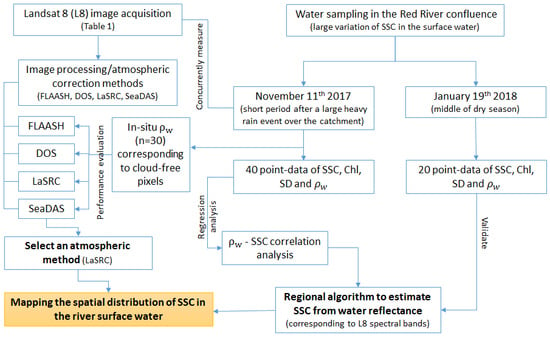
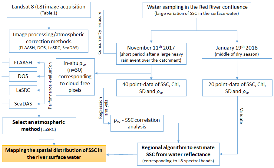
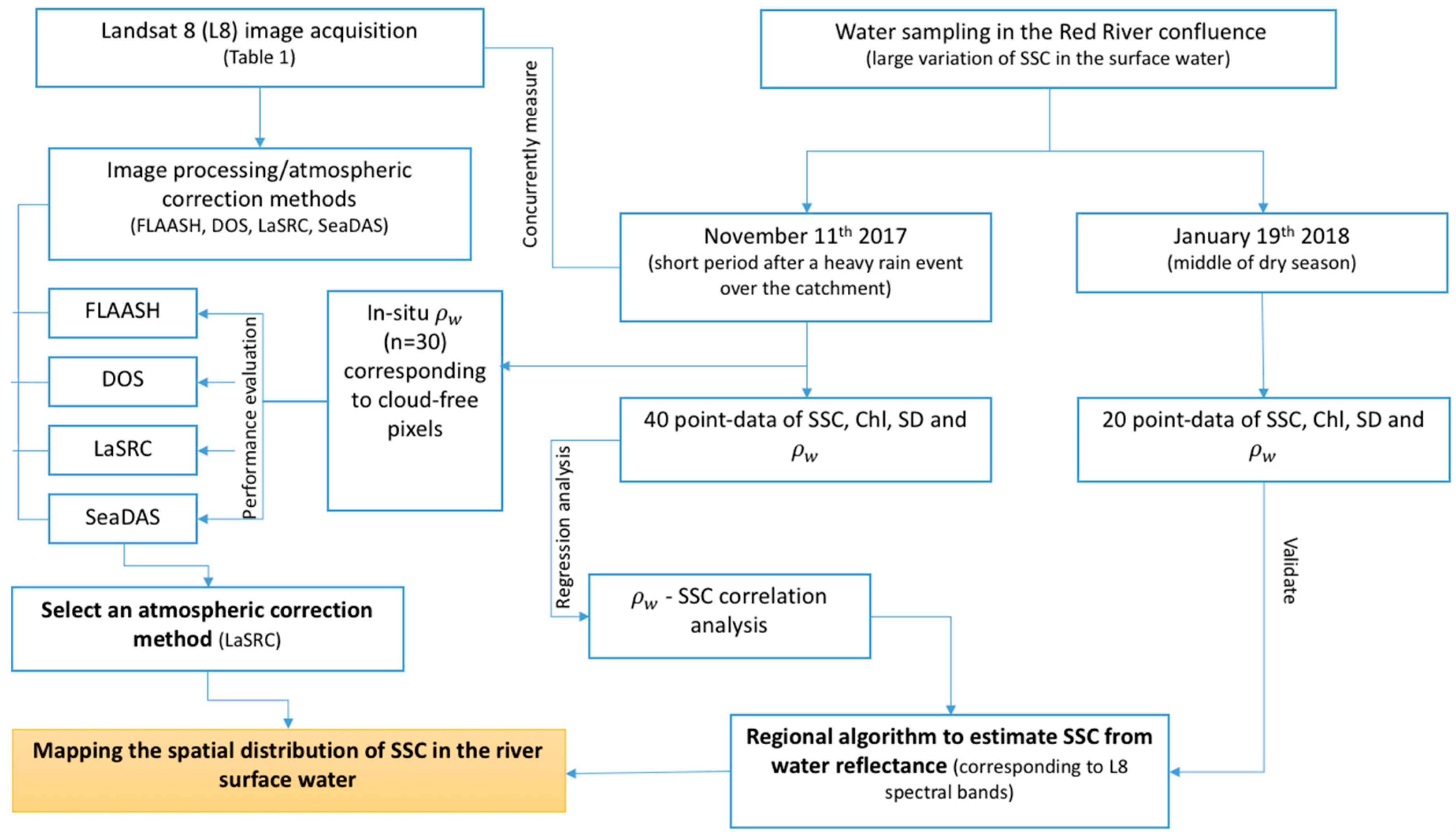
2. Materials and Methods
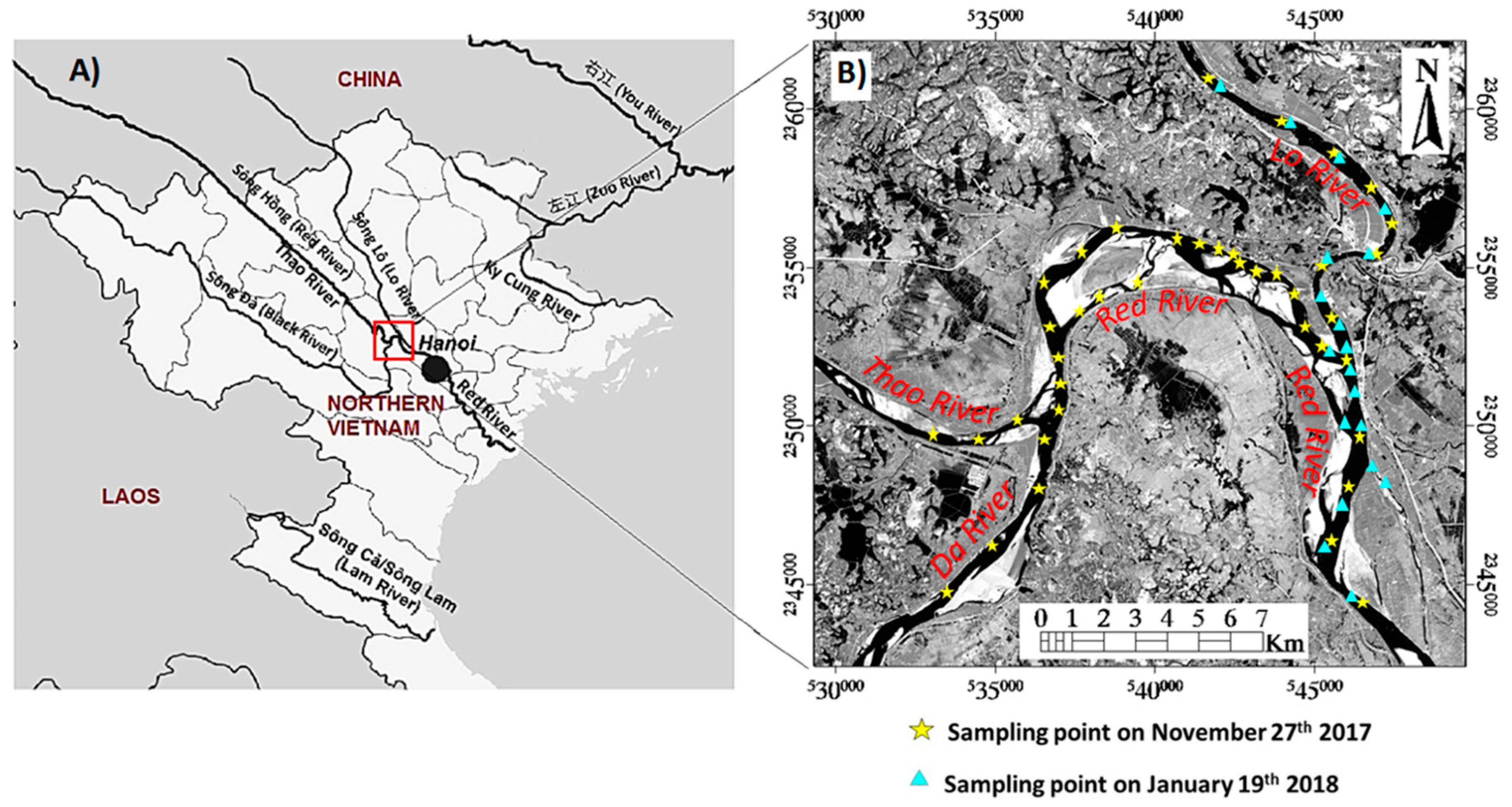
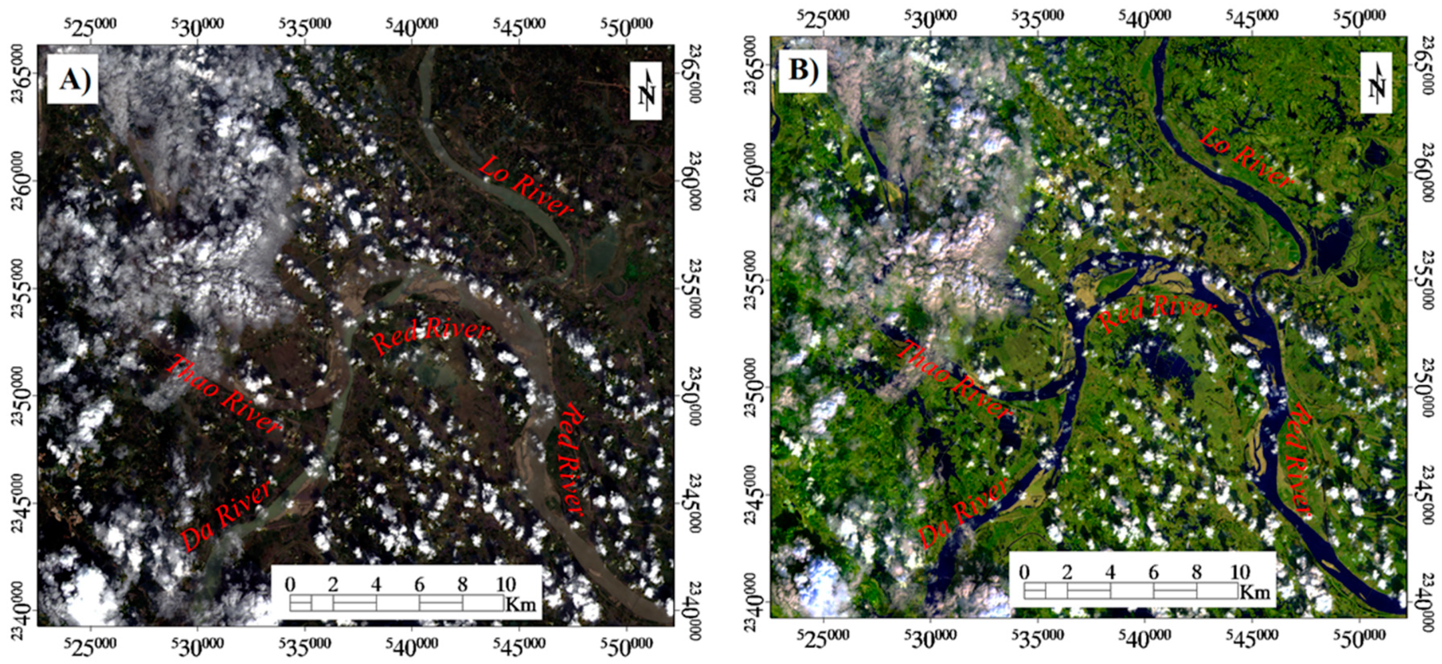
2.1. Study Area

The Red River is the second largest river in Vietnam, after the Mekong River in Southern Vietnam. It is a complex hydrological system that is strongly affected by anthropogenic activities [13]. The river is one of the most sediment-laden rivers in the world, with an estimated suspended load ranging from 90 × 106 ton/year [36] to 160 × 106 ton/year that discharge into the Gulf of Tonkin [12]. The Red River crosses into Vietnam at Ha Khau and Lao Cai named Thao River, and flows downstream. It receives inputs from two major tributaries, the Da and Lo rivers, in Thai Hoa commune (Ba Vi district, Hanoi city, Vietnam) and Bach Hac ward (Viet Tri, Phu Tho, Vietnam), respectively (Figure 1). It then flows eastward to the Gulf of Tonkin (the South China Sea). The river confluence, where three major tributaries intersect, is selected in this study because of its complexity in hydrodynamics and diversity in their optical properties. The river-bed from the sub-confluence of the Thao River and the Da River to the sub-confluence of the Red River with the Lo River, is approximately 4 m in width during the wet season, and 200–500 m in width for two channels in the dry season. The mean depth of these channels is 5–6 m in the dry season and may reach 10–11 m during the rainy season [37]. Mapping the distribution of SSC in this confluence helps us to better understand the contribution of each tributary in providing suspended load in the Red River.
In addition, the Red River is situated in the region that is affected by the tropical monsoon climate, which is characterized by the alternations between the dry and wet seasons. The wet season lasts for six months from May to October (recently, the season extents to November), and it accumulates approximately 85–95% of the total annual rainfall. The mean annual water discharges of the Da, Lo, and Thao rivers are 1700, 1050, and 750 m3/s (as calculated for the period from 1998–2008) [36], but due to the recent construction of dams on the Da River and the Lo, the mean annual water and suspended sediment discharges in these three tributaries have been drastically changed, i.e., the water discharges of all three tributaries have increased slightly in contrast to the downward trend of suspended sediment discharges in the Da River and the Red River [38]. The mountainous areas in the upstream basin of the Red River, particularly the Thao River, are highly eroded due to their tectonically active geologic settings [39]. The high-erosion rates give the river its red-brown color, making up the present-day name of the river. Additionally, the establishment and operation of two large reservoirs in the Da River (Hoa Binh and Son La hydropower reservoirs) has led to a considerable reduction in the total suspended load in the Red River [40]. The Thao River had been ranked as the second significant source of suspended sediment discharge among three tributaries prior to 1989, and it became the first significant source of suspended sediment discharge for the Red River from 1989 up to the present [38].

2.2. Field Sampling and Measurement

In situ SSC and above-water radiometric data were collected concurrently during the two field campaigns on 11 November 2017 (corresponding to late of the rainy season in 2017, after a short period of heavy rains over the catchment in October and early November 2017 [41]) and 19 January 2018 (middle of dry season). Water samples and water-leaving reflectance measurement were collected/recorded at 60 sites (Figure 1) within an hour before, and two hours after the L8 overpass time, i.e., ~10:30 a.m. local time) by two groups of three people in two boats. Water samples were taken at a depth of 0–50 cm using a Van Dorn water sampler, preserved in 1 L cleaned, dark-color bottles, and then refrigerated and transported to the laboratory.
Through the laboratory exercise, both chlorophyll a concentration (Chl) and SSC were determined following the standard methods described in the American Public Health Association [1]. Specifically, Chl was determined via spectrophotometric methods using acetone 95% extraction through a 0.7 μm porosity filter (using the Whatman 1825-047 GF/F Glass microfiber 47 mm diameter, 0.7 µm nominal pore size), and a DR 5000 UV-VIS Laboratory Spectrophotometer and SSC was determined by the standard gravimetric method. For SSC determination, water samples were filtered under a vacuum through a 1.5 μm mesh (using the Whatman 934-AH Glass microfiber 47 mm diameter, 1.5 µm nominal pore size). The filter pads were then flushed with distilled water and dried (at 104 ± 1 °C for a minimum of one hour). The SSC was then calculated using the following equation:
SSC = (A − B)/V,
where A is the mass of filter and dried residue (mg), B is the mass of filter (tare weight) (mg), and V is the volume of water sample filtered (L).
Above-water reflectance measurements were made at all the sites using a SVC (Spectra Vista Corporation, Poughkeepsie, NY, USA) GER1500, a field portable spectroradiometer covering the ultra-violet, visible, and near-infrared (NIR) wavelengths from 350 to 1050 nm at 1.5-nm resolution. The water-leaving reflectance, i.e., ρw(λ), was corrected for surface Fresnel reflection using the following Equation [42]:
ρw(λ) = Rp*{[Lw(λ)-ρ*Lsky(λ)]/π*Lp},
where Rp is the reflectance of our standard reference panel, Lw(λ) is the water-leaving radiance, Lsky(λ) is the sky radiance measured sequentially at 40–45 degrees from nadir and zenith, respectively, and 135 degrees from the Sun in azimuth [43], ρ is the air-water interface Fresnel reflectance with a value of 0.022, and Lp is the radiance for the reference panel.
Along with water sampling, water clarity was measured concurrently in the field using a standard 20 cm plastic Secchi disk. The Secchi Depth (SD) measurements were used in the field as a reference to exclude areas with potential effects of river bottom on ρw. Using ρw resampled to L8 spectral response functions [44] and measured SSC, we experiment with multiple empirical correlations to identify the most robust band (or band combinations) that best explains the variability in SSC in the Red River.

2.3. Image Analyses

The L8 images acquired on 11 November 2017 and other six images acquired in both wet and dry seasons of 2013, 2014, and 2017 were analyzed in this study. The image characteristics, including acquisition time, solar geometry, path/row, and environmental conditions are tabulated in Table 1.
We further evaluate the performances of the four atmospheric correction methods, i.e., LaSRC, DOS, FLAASH, and SeaDAS, using measured in situ ρw. The standard Landsat-8 surface reflectance products (ρwLaSRC) obtained from LaSRC data are readily available via the USGS Earth Explorer data portal [45]. The algorithm uses available ancillary data, the aerosol Moderate Resolution Imaging Spectroradiometer–Climate Modeling Grid–Aerosol Information as input data to correct for the effect of the atmosphere [46]. Furthermore, Level-1 TOA radiance/reflectance images were ingested into the ENVI 5.3 software package to gauge the performances of two commonly used atmospheric correction modules, FLAASH and DOS, to generate surface reflectance products, hereafter referred to as ρwFL and ρwDOS, respectively. Note that while TOA radiance was supplied to FLAASH, DOS applies TOA reflectance products to arrive at surface reflectance products. The DOS procedure uses the dark values associated with the minimum values of L8 image bands. For the implementation in FLAASH, the tropical atmospheric profiles were employed, together with a generic tropospheric aerosol layer. The over-water retrieval is carried out via identifying dark water pixels, followed by computing the reflectance ratio of the NIR and Short-wave Infrared (SWIR) bands (i.e., 2.2-micron channel), which was proven to yield reasonable estimates of water constituent in turbid waters in tropical area [47]. The SeaDAS package, originally developed for the atmospheric correction of ocean color images and recently adopted for processing L8 data, uses the Rayleigh-corrected NIR and SWIR (1.6-micron channel) band ratio to infer the dominant aerosol model and optical thickness [48]. Here, the SeaDAS-derived remote sensing reflectance products are converted to water-leaving reflectance (ρwSDS = Rrs × π) to allow for coherent inter-comparisons across different algorithms.
Matchup analyses were then conducted using the in-situ ρw (n = 30) collected on 11 November 2017 to assess the quality of various reflectance products. The detailed procedure of using L8 images for quantifying and mapping SSC in the Red River in this study is described in Figure 2.

3. Results

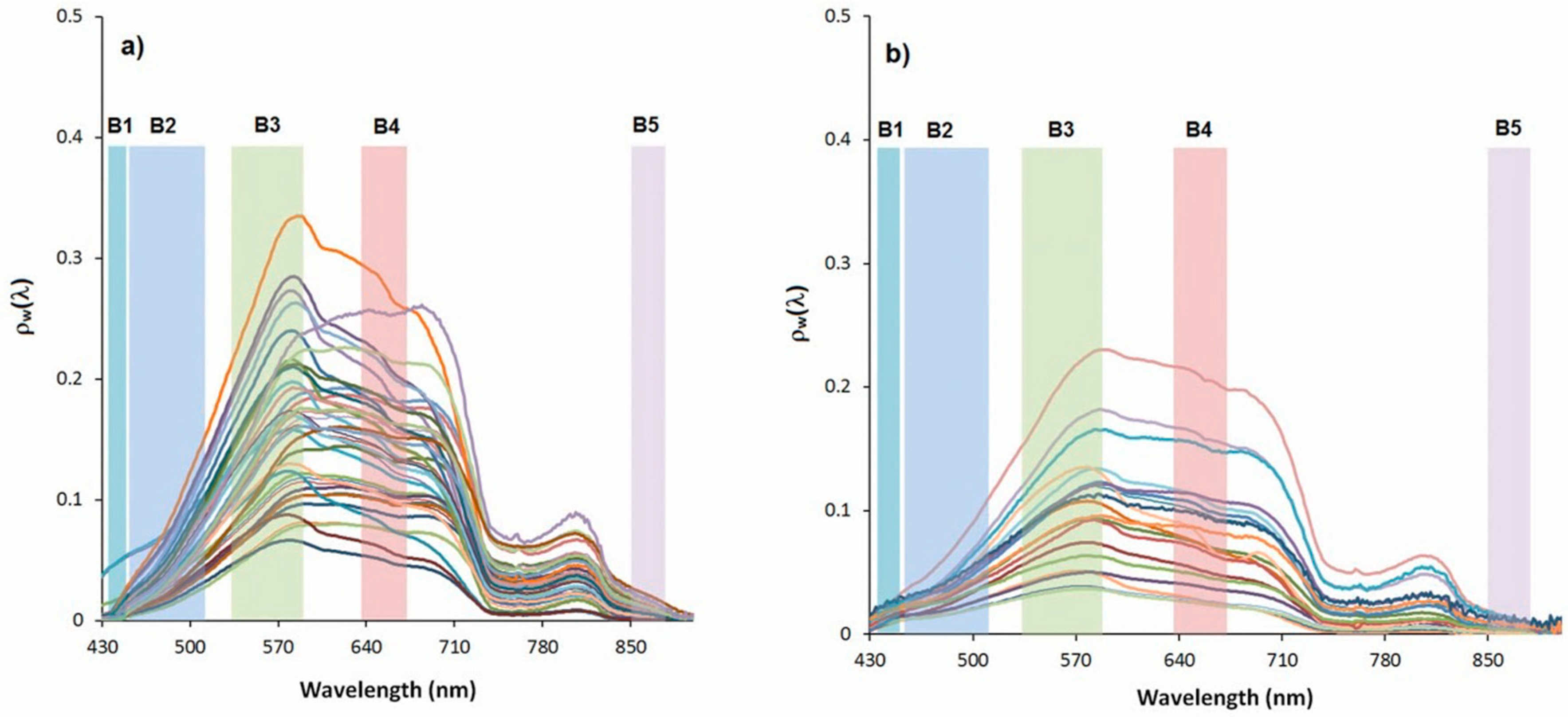
3.1. In Situ Radiometry and SSC

The measured ρw within the range of 400–900 nm associated with the 60 sites over the confluence of the Lo-Da-Thao rivers (Figure 1) are shown in Figure 3a,b for 11 November 2017 and 19 January 2018, respectively. The hyperspectral water-leaving reflectances in the confluence measured in November 2017 is slightly larger in magnitude than those measured in January 2018, indicating larger backscattering signals due to increased SSC in November 2017 (i.e., towards the end of rain season). This is corroborated by comparing in situ SSC data for the two campaigns, where mean SSC in November was nearly twice than that in January 2018 (i.e., 75.8 versus 46.4 mg/L in Table 2). The ρw are characteristic of highly turbid waters and are similar in shape and magnitude to previously reported spectra [7,49,50], with distinct increased water-leaving radiance within the red/NIR region, i.e., 650 to 670 nm. The higher variability in the spectral curves in Figure 3a within the 600–700 nm range reflects a larger variability in optically active constituents of the river waters in the wet season (prior to November) than in the dry season (after November). The differences in the shapes of the two timeframes can be attributed to distinct phytoplankton types and their specific absorption spectra. Furthermore, it is postulated that the differences in particulate (organic/inorganic) scattering/absorption properties may give rise to dissimilar ρw, i.e., flat spectra in dry season (Figure 3b) versus peaked spectra at ~570 nm. Further research is required to identify the specific inherent optical properties of water constituents in the Red River, to enable an enhanced understanding of contributions of various particles and/or phytoplankton types.
Table 2 includes the descriptive statistics associated with correlations among in situ SSC, SD, Chl, and L8 band-averaged reflectance spectra. SSC in the river water ranged widely from 22.4 to 178 mg/L (average value of 75.8 mg/L) in November 2017, and from 13.2 to 78.4 mg/L in January 2018 (average value of 46.4 mg/L). As expected, SSC is highly correlated with the SD with the Pearson coefficients, RSSC, of −0.94 and −0.77 in November and January, respectively. Contrary to SSC, Chl in the river water ranged from 1.3 to 56.1 mg/m3 (average of 12.6 mg/m3) in November 2017, approximately half of that in January 2018 (ranged from 6.7 to 90.3 mg/m3, average of 23.2 mg/m3). The correlation between SSC and Chl in the river water was found to be insignificant, ranging from −0.04 (for the dataset obtained in November 2017) to −0.68 (for the dataset obtained in January 2018), confirming the high complexity of the river water color in the wet season which varies largely within the tone from green (driven by Chl pigments) to brownish red (derived from Seston). Following several experiments, we found that SSC is correlated with ρw(865), with the coefficient of determination being 0.65, suggesting its high potential for predicting SSC in the Red River.
We then evaluated commonly used band ratios, such as ρw(865)/ρw(655), ρw(655)/ρw(562), ρw(482)/ρw(655), and ρw(443)/ρw(655) [22] to estimate SSC using the 40 in situ observations in November 2017. Results showed that SSC has a fairly strong correlation with three ratios, B4/B3, B4/B5, and B4/B2 (R2 = 0.75, 0.70, and 0.61, respectively) with B4/B1 exhibiting poor correlations (R2 = 0.04). The latter is not surprising because B1 is highly influenced by the dissolved organic absorption. Results obtained from the regression analysis of in situ SSC with B4/B3, B4/B2, B4/B5, and B5 for the 40 sampling points are illustrated in Figure 4a–d, respectively. The three band-ratio of Landsat data for estimating SSC has not been addressed in preceding studies [22]; only the combination of L8 bands 2, 3 and 4 have been examined recently [31,32]. Considering the effect of suspended matters on water spectrum, several L8 band combinations within the visible and NIR were investigated, i.e.: (B3 + B4)/B2; (B3 + B5)/B2; (B4 + B5)/B3; (B3 + B5)/B4; (B3 + B4)/B5. The (B4 + B5)/B3 exhibited a strong correlation with SSC (R2 = 0.76; Figure 4e), while both (B3 + B4)/B5 and (B3 + B5)/B4 were less correlated with SSC (R2 = 0.02 and 0.06, respectively), and the two other ratios of B2 ((B3 + B4)/B2 and (B3 + B5)/B2, respectively) showed moderate correlations with SSC. The L8 there-band combination for estimating SSC in a reservoir [24] was also explored and it is presented in Figure 4f, indicating the limitation of this band combination for estimating SSC in the highly turbid water, such as the Red River. The analyses suggest that exponential fits provide best estimates of SSC, which agrees with a previous study [51]. Among all the analyses, SSC in the Red River water is strongly associated with the B4/B3 and the (B4 + B5)/B3, i.e., ρw(655)/ρw(562) and [ρw(865) + ρw(655)]/ρw(562), with the similar highest determination of coefficients (R2 = 0.75 and 0.76) and the same smallest errors (root mean square errors, RMSE, of 0.31 mg/L and 0.305 mg/L, corresponding to <1% of mean). Thus, these band combinations are selected for estimating SSC in the Red River waters in this study using the following equation:
SSC = 2.73 × e3.11 × (B4/B3)
and:
SSC = 4.24 × e2.53 × [(B4 + B5)/B3]
where the SSC units are expressed is mg/L, B4/B3 is the ratio of ρw(655)/ρw(562) and (B4 + B5)/B3 stands for [ρw(865) + ρw(655)]/ρw(562).
We further validated the performance of the two models (Figure 4a,e) using the 20 measurements collected in 19 January 2018 (Figure 5a,b). The estimated SSC are relatively consistent with the in situ SSC, with a RMSE of 9.08 mg/L, R2 = 0.75 (Figure 5a), which corresponds to normalized RMSE of <20% given the mean SSC, i.e., 9.08/46.4. The uncertainties in the proposed model resemble the performance of another empirical models using L8 NIR band [28,52] and are lower than those utilizing machine learning methods [52]. Such relatively high uncertainties are expected, due to the lack of representativeness in ρw-SSC model development associated with the dry season. Such under-representation can be surmounted by incorporating the specific inherent optical properties of water constituents in model developments [53]. Yet, recognizing the uncertainties, the proposed empirical model can be applied in river water management practices to enable timely decision-making using L8 images. For example, using our model (Equation (3)), it would be possible to monitor illegal sand exploitation and/or waste-water discharges through identifying anomalous spatial patterns in Landsat-derived SSC.

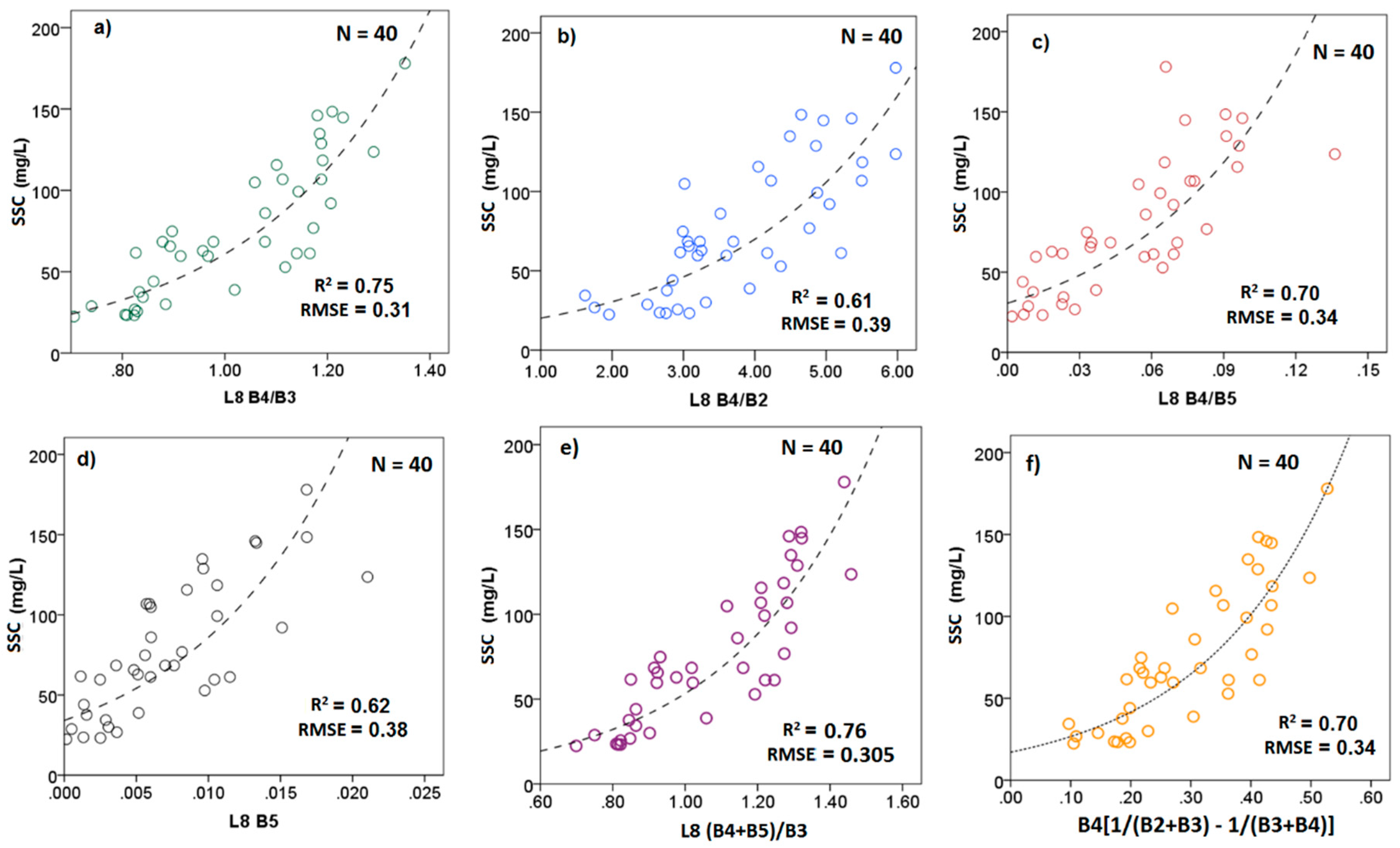
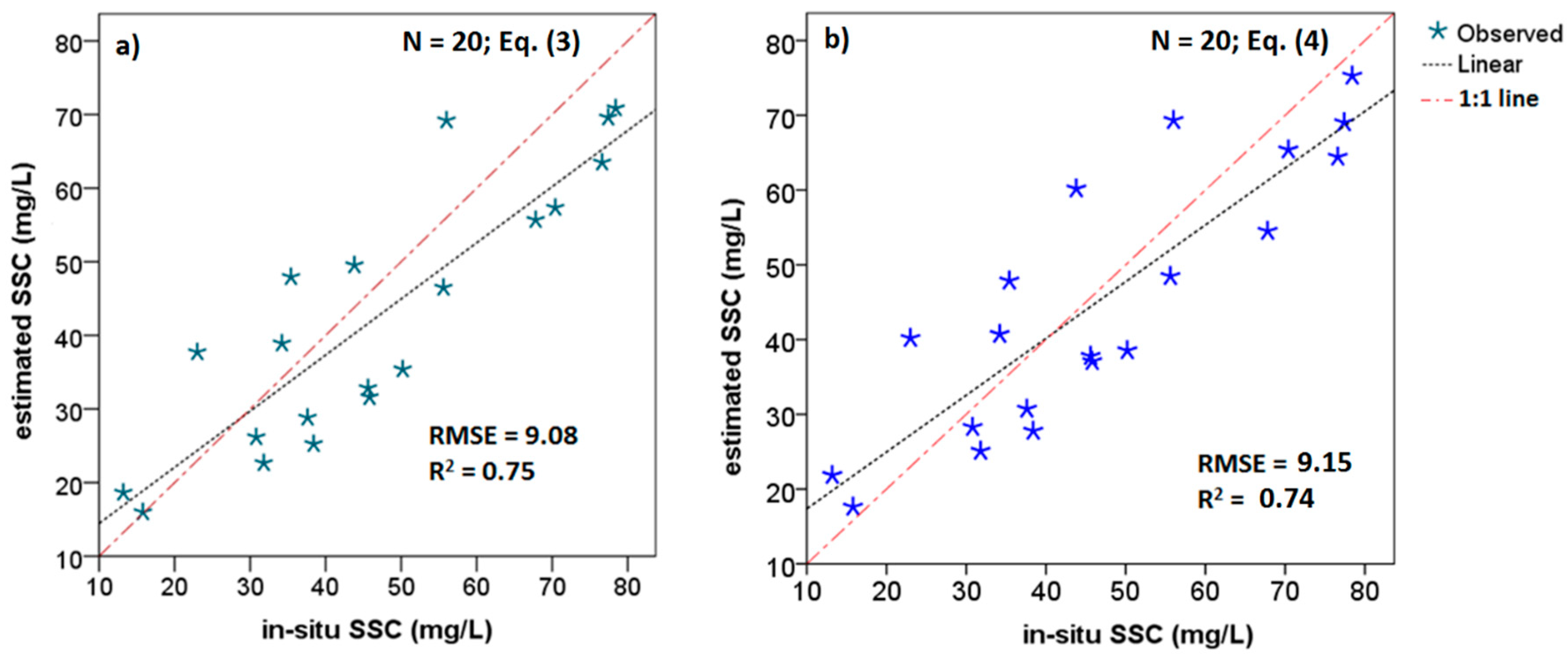
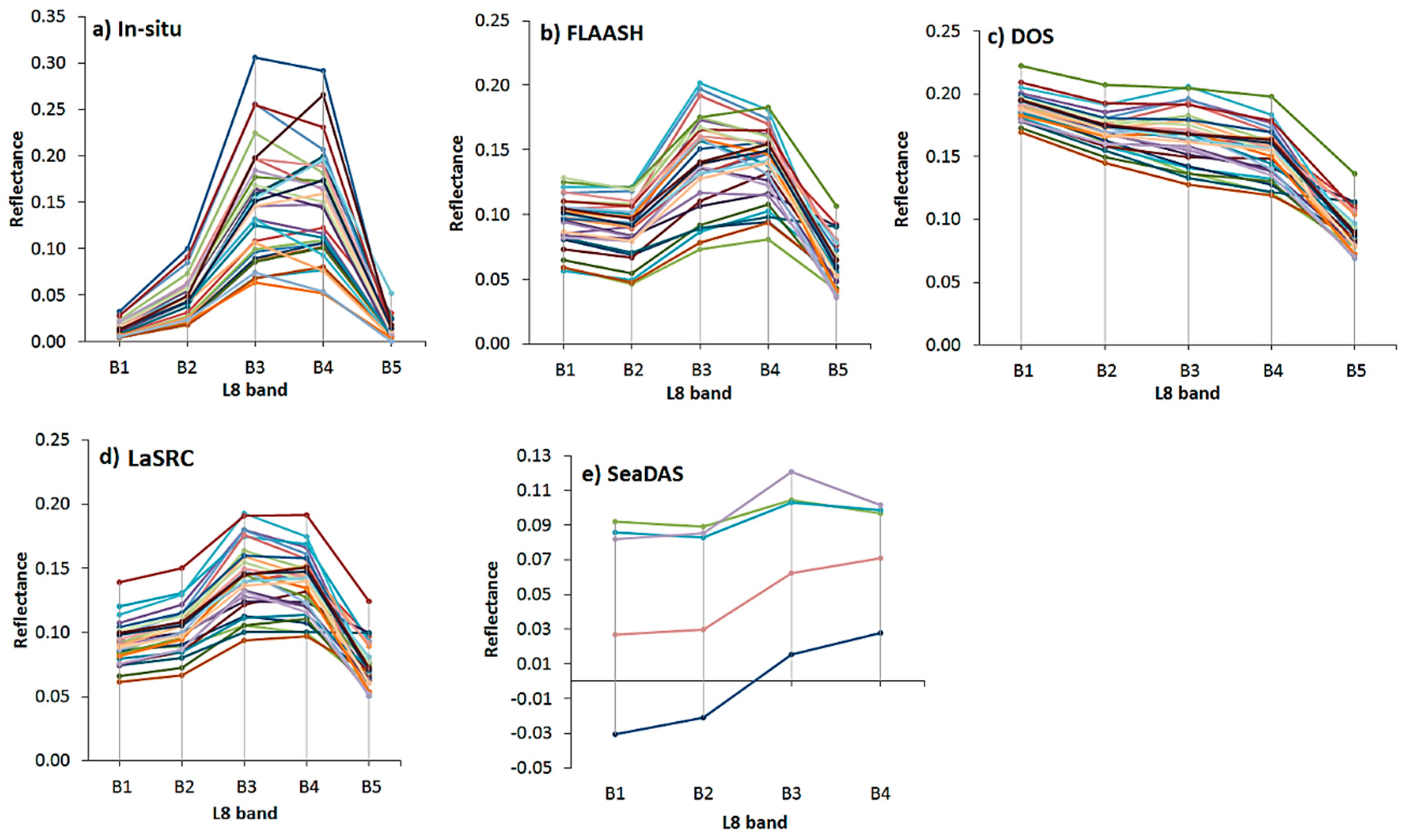
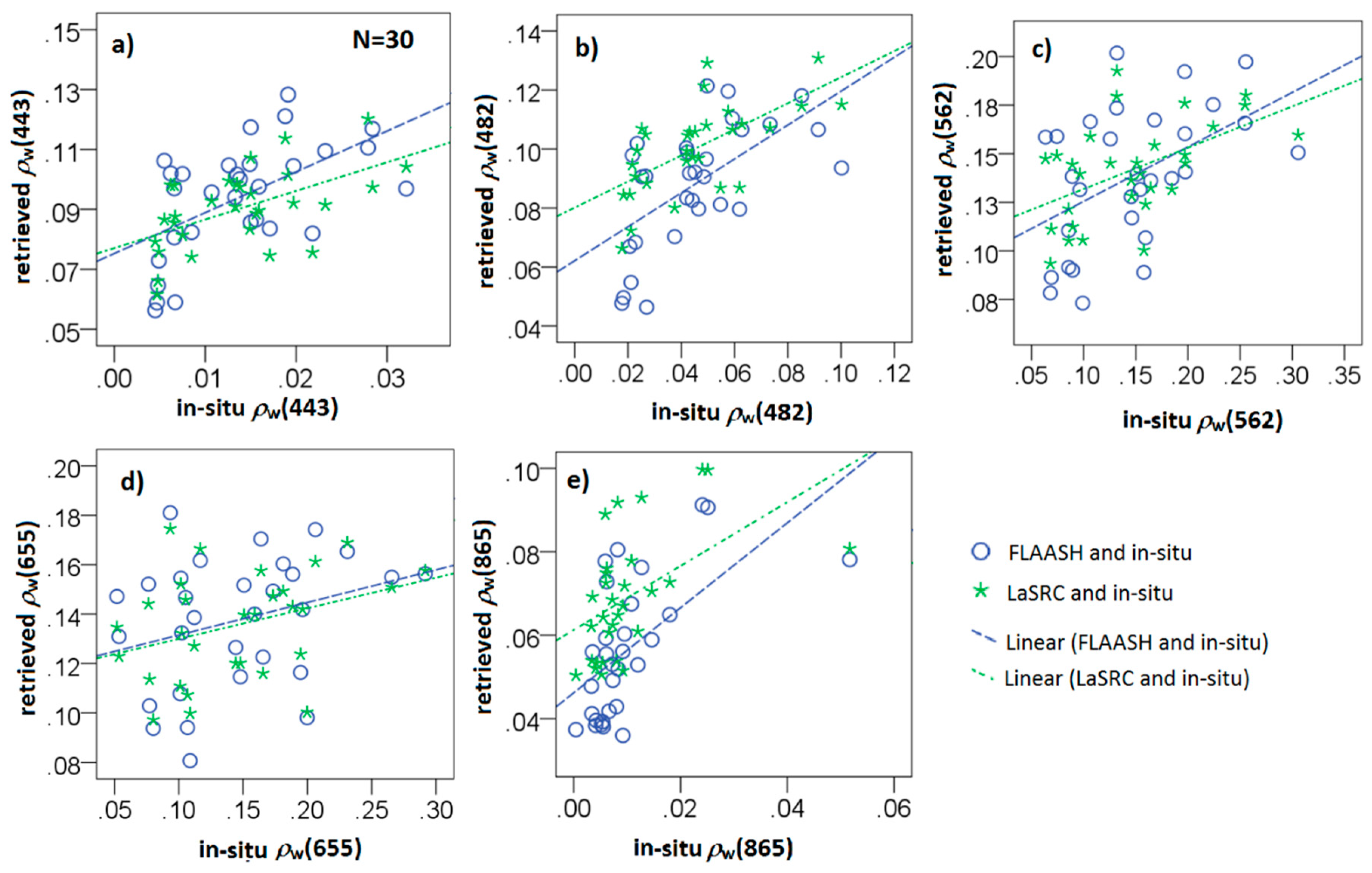
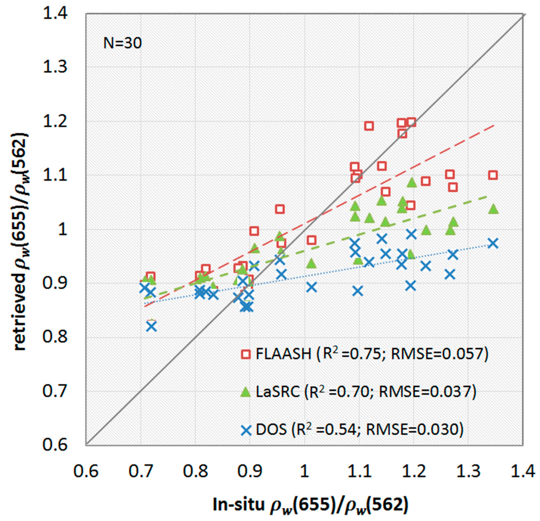
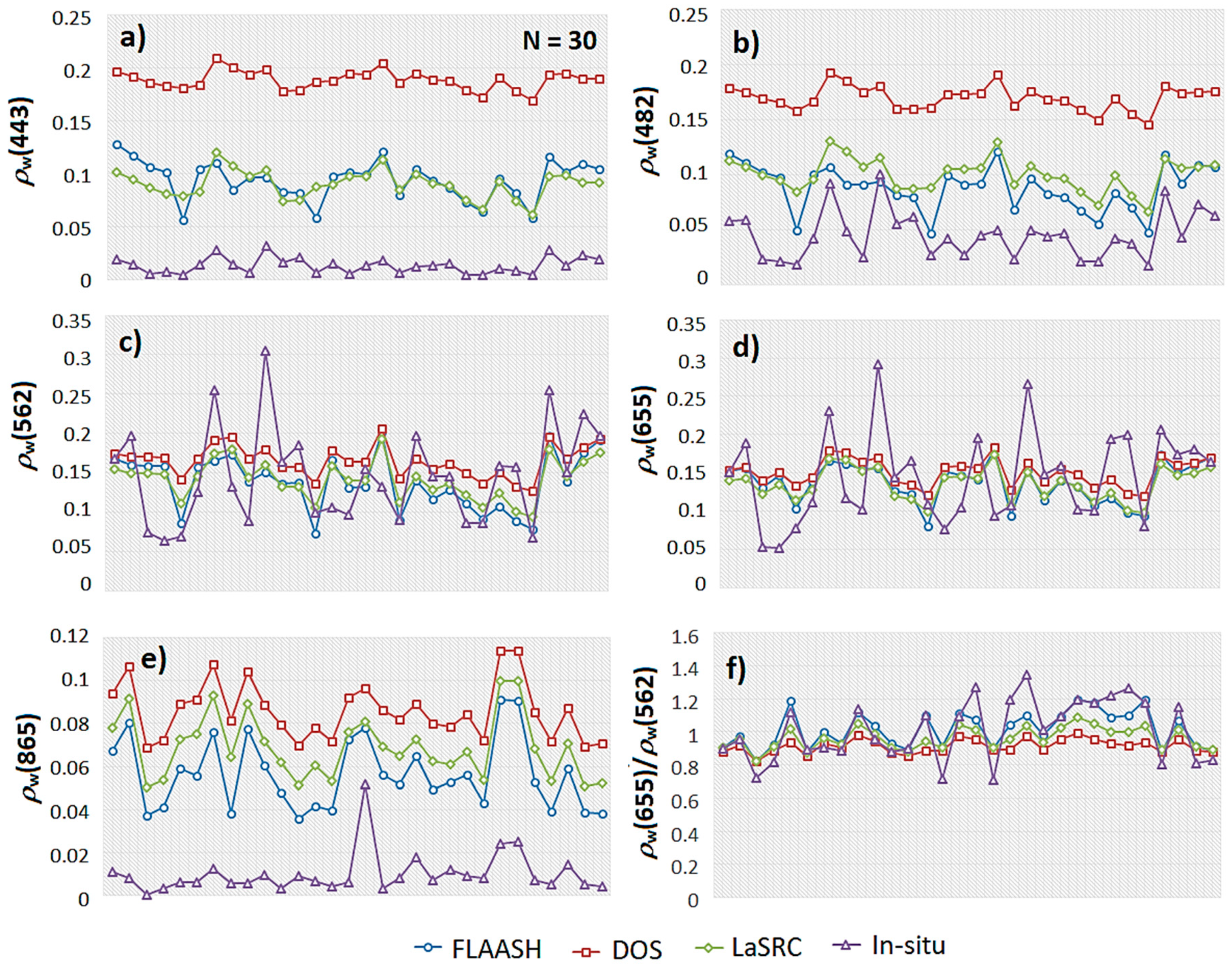
3.2. Evaluating of Landsat-Derived ρw for Monitoring SSC

The natural-look image Figure 6A and the false color composition image Figure 6B of the confluence on 11 November 2017, which reflects the challenging environmental conditions, is illustrated in Figure 6. Due to the presence of scattered clouds or their shadows, only 30 in situ samples were used for matchup analyses.
The four different ρw products are derived from LaSRC (i.e., USGS standard products [35]), DOS, FLAASH, and SeaDAS. Figure 7 shows a qualitative comparison of spectral profiles of ρw obtained from the four processors (Figure 7b–e) and the in situ data. It can clearly be seen that none of the processors provides robust retrievals of ρw. The retrieved spectra are different from the in situ data, both in their shape and magnitude. Owing to the presence of adjacent clouds and its strict flagging criteria, SeaDAS mostly did not yield valid retrievals. SeaDAS also uses the NIR channel to estimate aerosol contribution; hence, no retrievals are reported for this channel. Furthermore, because of relatively high backscattering in the NIR, ~30% of SeaDAS retrievals were physically unrealistic (i.e., negative in the blue bands) one of which is shown in Figure 7e.
Table 3 illustrates the statistical analyses for the performances of different processors. The statistical metrics include descriptive statistics of L8 retrievals and their linear regression analysis parameters with in situ ρw (R2, RMSE, slope, and y-intercept). Because of inadequate valid retrievals and lack of rigor in the performances (Figure 7c), the results of SeaDAS and DOS are excluded in the table. The computed metrics indicate that outputs of LaSRC and FLAASH significantly overestimate ρw in all bands (Figure 8). However, on average, they produce reasonable ρw in B4, and in particular, in B3 (Figure 8d,c). The computed R2, ranging from 0.09 to 0.41, suggests that the L8-derived single band reflectance for SSC retrievals may be limited, due to large uncertainties in the atmospheric correction methods (Table 3). Nevertheless, the band ratio B4/B3 derived from LaSRC and FLAASH processing exhibits reasonable correlations with in situ SSC data, i.e., R2 = 0.7 for LaSRC and R2 = 0.75 for FLAASH (Figure 9). This implicates that the band ratio model is less subject to errors in the atmospheric correction (e.g., inaccurate estimations of aerosol type). Figure 9 further indicates that the deviations from the linear fits become larger in water types where ρw(655) > ρw(562), i.e., sediment-dominated scattering waters, and that the sensitivity of the band-ratio model to uncertainties in different processors is similar for (ρw(655)/ρw(562)) < 0.9 as the linear fits converge towards smaller fractions.

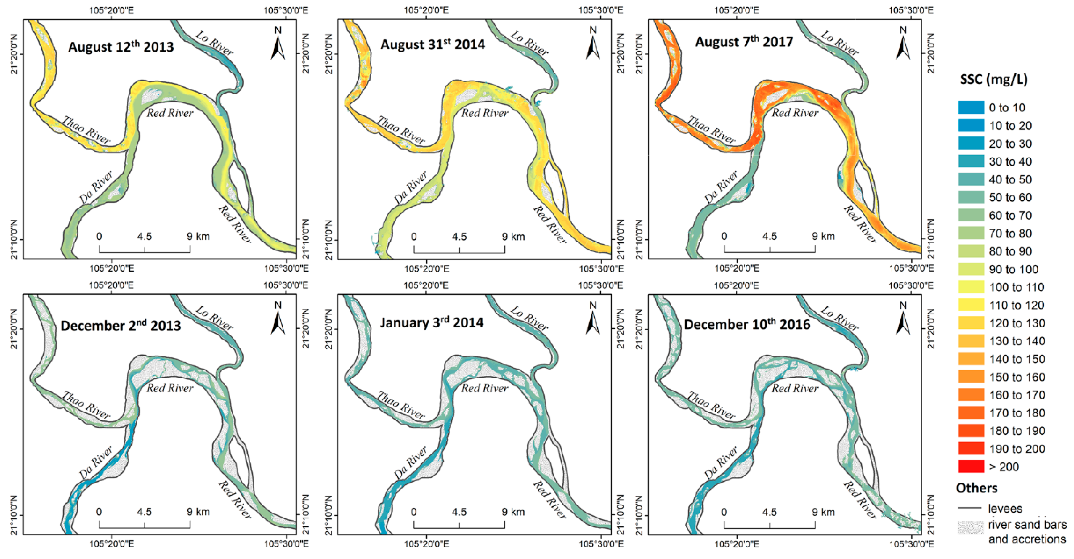
3.3. Mapping SSC in the Red River Using L8SR

Since the derived B4/B3 model (Equation (3)) from the standard L8 USGS products (L8SR) exhibit highest agreements with in situ measurements, and they are readily available via the EarthExplorer [45]; therefore, we apply this empirical model (Equation (3)) to arrive at the spatial distributions of SSC along the Red River. we further evaluated L8SR products retrieved from six cloud-free L8 scenes (Table 1) acquired in the wet (November/August) and dry seasons (December/January). Figure 10 shows the spatial distributions of estimated SSC in the Red River waters in space and time. The estimated SSC in the Red River water ranged from 4.0 mg/L to 200 mg/L (mean value of 85 mg/L) in the rainy season, which is twice as high as in the dry season (from 4.5 mg/L to 60 mg/L; mean value of 43 mg/L). Regarding its spatial distribution, the SSC was found to be higher in the Thao River; in particular, towards the north bank of the Red River (Figure 10). The SSC is, however, lower in the Lo River and the Da River in both seasons (Figure 10). The trend in the distribution can be seen in all the maps, but much more evidently in the estimated SSC in the wet season (Figure 10 top row).
The spatial distribution of SSC in Figure 9 indicates that the Thao River is a major source of suspended sediment for the Red River. This result is in agreement with the suspended sediment budget estimated from daily field monitoring and water discharges at the hydro-climatic stations, namely, Yen Bai and Lao Cai on the Thao River, Hoa Binh on the Da River, Vu Quang on the Lo rivers, and Son Tay, Ha Noi on the Red River [41], and the preceding studies [13,36]. The Da River was recognized as the primary source of suspended load for the Red River in the period of 1958 to 1995 [54,55]; however, this study suggests that the Da River is no longer a major source for the Red River compared to the Thao River. The impact of the hydropower dam systems on the Da River and the Lo River on the suspended load capacity of the Red River, which has been demonstrated in previous studies [13,36,38], has also been verified using L8 images. In particular, the Thao River, within the Vietnamese territory, has the smallest catchment area (12,000 km2) compared to that of the Lo River (22,000 km2) and the Da River (26,800 km2) but it provides the largest suspended sediment source to the Red River, compared to the other two. This is a consequence of sediment impoundment in the hydropower-dams on the Da River (seven operating dams) and the Lo River (nine operating dams). The SSC in the Lo River water is rather low compared to the other two tributaries, the Thao River and the Da River, in both seasons, illustrating the minor role of Lo River in providing suspended load for the Red River [36]; although the Lo River has a large catchment area that has been excessively exploited for agriculture and other long-term surface erosion activities.
In this study, the Red River reflects a typical characteristic of tropical river systems, where most of the suspended load is discharged during the rainy season [10]. This trend is observed in Figure 10 through two features: (a) the wider reach in the rainy season, corresponding to a high amount of run-off water discharge, (b) the higher SSC levels corresponding to high suspended sediment discharge. Similarly, with the smaller area of water surface in the dry season, a lower SSC level is found (correlation coefficient, R, of total surface water area, and mean value of SSC in six maps within Figure 9 is 0.85). Obviously, run-offs and the accompanied top-soil erosion of materials is a major factor that controls the distribution and variation of SSC in the Red River water in space and time.

4. Discussion

The remote sensing algorithms developed for SSC retrievals have long been utilized for various science and application areas [6]. The models for estimating SSC can be clustered into two groups: (a) statistical techniques such as machine learning and (b) empirical methods based on the relationship between SSC and water-leaving reflectance [52]. As recognized by previous studies, algorithms for SSC retrievals based upon SSC-reflectance relationships are more robust than those derived from statistical models [28]. Unlike coastal waters and lake waters, which mostly contain mineral particles and organic matters, suspended sediment in river waters is composed of several components, such as mineral particles, organic substances, pollutants, and sewage effluent, which result from erosion, transport, and deposition processes occurring within the catchments. As a consequence, the optical properties of river waters vary, depending on the response of the optical active constituent of the water column (e.g., mineral particles, CDOM or Chl, listed in Table 2).
Preceding studies have indicated that the suitability of the L8’s NIR band retrieved reflectance [28,52] or in situ ρw(860) [53] for estimating SSC in river water. The high correlations in in situ ρw(865) and SSC obtained from the Red River in the two different surveyed times (Table 2) also confirm the high potential of the L8 NIR band reflectance for estimating SSC in the river water. However, the use of a single band algorithm for a SSC estimate is challenging, due to the effects of the atmosphere on the water-leaving reflectance in visible/NIR region [28], and of the sediment type and particle size on water-leaving reflectance, particularly in highly turbid waters [53]. In Figure 8e, we demonstrate the large uncertainties in the retrieved ρw(865), which may lead to the overestimation of SSC in the Red River. To further provide evidence on the effects of atmosphere, the in situ and retrieved ρw at each site (n = 30) are compared in Figure 11. The retrievals in the ρw(443), ρw(482), and ρw(865) are often overestimated. The retrievals in the green and red channels, on average, follow the same pattern, however, they fail to capture the associated dynamic ranges, implicating uncertainties in estimated SSC level when using single-band methods (Figure 11c,d).
Furthermore, the use of the spectral band-ratio in estimating water constituents has proven to reduce the dependency on the suspended sediment type and particle size [39]. Figure 8 shows the comparison of the spectral band ratios retrieved using different atmospheric correction methods. According to R2 values, the uncertainties in the single-band reflectance in the green (R2 = 0.18 to 0.27) and the red (R2 = 0.09 to 0.17) regions have been improved by using these two-band ratios (R2 = 0. 54 to 0.75). The appropriateness of the band ratio of red-green used to develop algorithm for estimating SSC agrees with empirical and semi-analytical spectral reflectance models for SSC estimates [56], and confirms that the band ratio of red-green is the best predictor variable for estimating SSC in dynamic waters using the statistical modelling method.
It is important to recognize that the river is a very dynamic system, which contains water, sediment, aquatic organisms, and other discharged materials on the way from the headwaters toward the sea [57]. The spot-sampling of SSC and water volume along the Red River, as part of the hydrological monitoring network, may help one to predict the river suspended load, but it is inadequate for understanding the river system dynamics for better management [58]. The use of appropriate satellite data products in combination with our validated regional algorithm, i.e., Equation (3), provides spatio-temporal SSC patterns that support rapid detections of anomalies in the distribution of SSC, which may be caused by human activities, such as flood discharging from on-river hydropower dams, and illegal river bottom sand exploitation. Therefore, the uncertainty of Equation (3) (normalized RMSE < 20%), which is lower than the error that is reported by statistical modelling techniques [52], is reasonable when applying it to the Red River. Furthermore, the wide range of SSC that is employed to develop the algorithm (from 22.4 mg/L to 178 mg/L) ensures its applicability in both dry and rainy seasons at local hydrological stations [41]. These products will help reduce the uncertainty associated with the seasonal time-lagged SSC level in the estimates. However, for monitoring higher SSC levels (>200 mg/L), which often occurs in the river water during flood events, future studies including more in situ SSC and ρw in flooded areas should be carried out in order to extend the range of SSC that is detectable by our proposed model.
The methods outlined in this paper could be applied to map SSC in the Red River system or in other rivers, but the specific coefficients of the algorithm (Equation (3)) needs be revised to match the optical characteristics of the SSC present in the target river waters. For instance, the algorithm should be re-calibrated to suit extremely turbid waters, i.e., >1000 mg/L [42], in the Red River that may occur due to flooding, multidate heavy rains, or dam failure. On the other hand, the revisit cycle of L8, 16 days, is not suitable for monitoring the dynamics of the Red River, particularly for river water in the tropical regions because of frequent cloud cover. For example, during July 2017 and July 2018, the Hoa Binh dam on the Da River (near the river confluence in our study area) discharged a significant amount of water to ensure dam security during flood events [60,61]. However, all of the L8 scenes acquired over the study area during July 2017 and July 2018 area were mostly covered by clouds, with the coverage ranging from 71% to 83%. Therefore, the map reflecting the dam’s discharge is still missing. When Landsat-9 and Sentinel-2C are launched within the 2021–2023 timeframe, combined with existing L8 and Sentinel-2A/B [62], the revisit time will significantly be improved, i.e., near daily, on average. Only within that timeframe, will it be possible to explore the utility of SSC retrievals during flood events. Our upcoming work will focus on collecting in situ data across a large extent of the Red River system and exploiting other optical satellite data for better monitoring of SSC over the Red River system using free, open-source remote sensing data.

5. Summary and Conclusions

This study demonstrates the high possibility of L8 data products for quantifying and mapping SSC in surface waters of a river in a tropical region with a large heterogeneity in SSC levels and optically active water constituent proportions, the Red River. To summarize, we found that (1) SSC in the Red River exponentially correlates with the green-red band ratio (R = 0.86), which yields retrievals of SSC with a normalized RMSE of ~ 20 %; (2) Comparisons of water-leaving reflectances produced from FLAASH, LaSRC, SeaDAS, and DOS atmospheric correction methods with near-concurrent in situ ρw, revealed a lack of rigor in all of the approaches (e.g., RMSE > 0.018 in ρw (562)). Nevertheless, it was found that the L8-derived green–red band ratio is minimally susceptible to uncertainties in the atmospheric correction allowing for its utility for river water management. Thus, due to their ease of access via US Geological Survey web portals, the standard land surface reflectance products were utilized for mapping SSC; (3) Maps of SSC distribution in the Red River waters indicated that the Thao River is the major source of sediment amongst the three tributaries in delivering suspended loads to the Red River, and the seasonal variation in SSC is highly related to the seasonal variation in run-offs (R = 0.85). We further conclude that these products and the methodology outlined in this paper could be applied to map SSC in highly turbid waters, which has similar optical characteristics and SSC range. The persistent presence of clouds in the tropical regions poses major challenges in the utility of Landsat data for monitoring SSC. Therefore, in the future, both (publicly free) Landsat and Sentinel-2 data generated via an identical processing chain should be explored, to gauge the use of multi-mission, moderate-resolution satellite images for monitoring SSC in extremely turbid, tropical riverine systems at relatively high frequency rates.

Author Contributions

Conceptualization, Q.V.P., N.T.T.H. and N.P.; formal analysis: Q.V.P., N.T.T.H. and L.T.O.; investigation, Q.V.P., N.T.T.H., T.B.N., N.T.N., L.T.O.; writing—original draft preparation, Q.V.P., N.T.T.H.; writing—review and editing, N.T.T.H. and N.P.; funding acquisition, Q.V.P.

Funding

This research was funded by THE VIETNAM NATIONAL SPACE SCIENCE AND TECHNOLOGY PROGRAM 2016–2020 (CNVT/16-20), project code VT-UD.02/16-20. Nima Pahlevan is funded under NASA ROSES #NNX16AI16G and USGS Landsat Science Team Award #140G0118C0011.

Acknowledgments

The authors gratefully acknowledge the support provided by the project code VT-UD.02/16-20 of the Vietnam National Space Science and Technology Program 2016–2020 (CNVT/16-20). The authors also thank the U.S. Geological Survey and NASA for providing the L8SR and other Landsat data.

Conflicts of Interest

The authors declare no conflict of interest.

References

  1. Clesceri, L.S.; Greenberg, A.E.; Eaton, A.D. Standard Methods for the Examination of Water and Wastewater, 20th ed.; APHA American Public Health Association: Washington, DC, USA, 1998; 1220p. [Google Scholar]
  2. Edward, T.K.; Glysson, G.D.; Guy, H.P.; Norman, V.W. Field Methods for Measurement of Fluvial Sediment. Available online: https://pubs.er.usgs.gov/publication/ofr86531 (accessed on 29 September 2018).
  3. Ritchie, J.C.; Cooper, C.M. Comparison of measured suspended sediment concentrations with suspended sediment concentrations estimated from Landsat MSS data. Remote Sens. 1988, 9, 379–387. [Google Scholar] [CrossRef]
  4. Doxaran, D.; Froidefond, J.M.; Castaing, P. A reflectance band ratio used to estimate suspended matter concentrations in sediment-dominated coastal waters. Int. J. Remote Sens. 2002, 23, 5079–5085. [Google Scholar] [CrossRef]
  5. Wang, J.J.; Lu, X.X.; Liew, S.C.; Zhou, Y. Retrieval of suspended sediment concentrations in large turbid rivers using Landsat ETM+: An example from the Yangtze River, China. Earth Surf. Process. Landf. 2009, 34, 1082–1092. [Google Scholar] [CrossRef]
  6. Ritchie, J.C.; Schiebe, F.R.; Mchenry, J.R. Remote sensing of suspended sediments in surface waters. Photogramm. Eng. Remote Sens. 1976, 42, 1539–1545. [Google Scholar]
  7. Wu, J.L.; Ho, C.R.; Huang, C.C.; Srivastav, A.L.; Tzeng, J.H.; Lin, Y.T. Hyperspectral sensing for turbid water quality monitoring in freshwater rivers: Empirical relationship between reflectance and turbidity and total solids. Sensors 2014, 14, 22670–22688. [Google Scholar] [CrossRef] [PubMed] [Green Version]
  8. Fan, C. Spectral analysis of water reflectance for hyperspectral remote sensing of water quality in estuarine water. J. Geosci. Environ. Protect. 2014, 2, 19. [Google Scholar] [CrossRef]
  9. Sathyendranath, S. Remote Sensing of Ocean Colour in Coastal, and Other Optically-Complex, Waters. IOCCG Report Number 3, Dartmouth, Canada, 2000, 140p. Available online: http://www.ioccg.org/reports/report3.pdf (accessed on 9 November 2018).
  10. Doxaran, D.; Babin, M.; Leymarie, E. Near-infrared light scattering by particles in coastal waters. Opt. Express 2007, 15, 12834–12849. [Google Scholar] [CrossRef] [PubMed]
  11. Astoreca, R.; Doxaran, D.; Ruddick, K.; Rousseau, V.; Lancelot, C. Influence of suspended particle concentration, composition and size on the variability of inherent optical properties of the Southern North Sea. Cont. Shelf Res. 2012, 35, 117–128. [Google Scholar] [CrossRef]
  12. Milliman, J.D.; Meade, R.H. World-wide delivery of river sediment to the oceans. J. Geol. 1983, 91, 1–21. [Google Scholar] [CrossRef]
  13. Le, T.P.Q.; Garnier, J.; Gilles, B.; Sylvain, T.; Minh, C.V. The changing flow regime and sediment load of the Red River, Viet Nam. J. Hydrol. 2007, 334, 199–214. [Google Scholar] [CrossRef]
  14. Wang, J.J.; Lu, X.X. Estimation of suspended sediment concentrations using Terra MODIS: An example from the Lower Yangtze River, China. Sci. Total. Environ. 2010, 408, 1131–1138. [Google Scholar] [CrossRef] [PubMed]
  15. Espinoza Villar, R.; Martinez, J.M.; Texier, M.L.; Guyot, J.L.; Fraizy, P.; Meneses, P.R.; Oliveira, E. A study of sediment transport in the Madeira River, Brazil, using MODIS remote-sensing images. J. S. Am. Earth Sci. 2013, 44, 45–54. [Google Scholar] [CrossRef]
  16. Mangiarotti, S.; Martinez, J.M.; Bonnet, M.P.; Buarque, D.C.; Filizola, N.; Mazzega, P. Discharge and suspended sediment flux estimated along the mainstream of the Amazon and the Madeira Rivers (from in situ and MODIS Satellite Data). Int. J. Appl. Earth Obs. Geoinf. 2013, 21, 341–355. [Google Scholar] [CrossRef] [Green Version]
  17. Aranuvachapun, S.; Walling, D.E. Landsat-MSS radiance as a measure of suspended sediment in the lower Yellow River (Hwang Ho). Remote Sens. Environ. 1988, 25, 145–165. [Google Scholar] [CrossRef]
  18. Mertes, L.A.K.; Smith, M.O.; Adams, J.B. Estimating suspended sediment concentrations in surface waters of the Amazon River wetlands from Landsat images. Remote Sens. Environ. 1993, 43, 281–301. [Google Scholar] [CrossRef]
  19. Zhang, M.; Dong, Q.; Cui, T.; Xue, C.; Zhang, S. Suspended sediment monitoring and assessment for Yellow River Estuary from Landsat TM and ETM+ imagery. Remote Sens. Environ. 2014, 146, 136–147. [Google Scholar] [CrossRef]
  20. Montanher, O.C.; Novo, E.M.L.M.; Barbosa, C.C.F.; Renno, C.D.; Silva, T.S. Empirical models for estimating the suspended sediment concentration in Amazonian white water rivers using Landsat 5/TM. Int. J. Appl. Earth Obs. Geoinf. 2014, 29, 66–77. [Google Scholar] [CrossRef]
  21. Pereira, L.S.F.; Andes, L.C.; Cox, A.L.; Ghulam, A. Measuring suspended-sediment concentration and turbidity in the middle Mississippi and lower Missouri Rivers using Landsat data. J. Am. Water Resour. Assoc. 2018, 54, 440–450. [Google Scholar] [CrossRef]
  22. Gholizadeh, M.H.; Melesse, A.M.; Reddi, L. A comprehensive review on water quality parameters estimation using remote sensing techniques. Sensors 2016, 16, 1298. [Google Scholar] [CrossRef] [PubMed]
  23. Pahlevan, N.; Lee, Z.; Wei, J.; Schaaf, C.B.; Schott, J.R.; Berk, A. On-orbit radiometric characterization of OLI (Landsat-8) for applications in aquatic remote sensing. Remote Sens. Environ. 2014, 154, 272–284. [Google Scholar] [CrossRef]
  24. Zheng, Z.; Li, Y.; Guo, Y.; Xu, Y.; Liu, G.; Du, C. Landsat-based long-term monitoring of total suspended matter concentration pattern change in the wet season for Dongting Lake, China. Remote Sens. 2015, 7, 13975–13999. [Google Scholar] [CrossRef]
  25. Alcântara, E.; Curtarelli, M.; Stech, J. Estimating total suspended matter using the particle backscattering coefficient: Results from the Itumbiara hydroelectric reservoir (Goiás State, Brazil). Remote Sens. Lett. 2016, 7, 397–406. [Google Scholar] [CrossRef]
  26. Hariyanto, T.; Krisna, T.C.; Pribadi, C.B.; Anwar, N. Development of Total Suspended Sediment Model using Landsat-8 OLI and In-situ Data at the Surabaya Coast, East Java, Indonesia. Indones. J. Geogr. 2017, 49, 73. [Google Scholar] [CrossRef]
  27. Quang, N.H.; Sasaki, J.; Higa, H.; Huan, N.H. Spatiotemporal Variation of Turbidity Based on Landsat 8 OLI in Cam Ranh Bay and Thuy Trieu Lagoon, Vietnam. Water 2017, 9, 570. [Google Scholar] [CrossRef]
  28. Yepez, S.; Laraque, A.; Martinez, J.M.; Sa, J.D.; Carrera, J.M.; Castellanos, B.; Lopez, J.L. Retrieval of suspended sediment concentrations using Landsat-8 OLI satellite images in the Orinoco River (Venezuela). C. R. Geosci. 2018, 350, 20–30. [Google Scholar] [CrossRef]
  29. Qiu, Z.; Xiao, C.; Perrie, W.; Sun, D.; Wang, S.; Shen, H.; He, Y. Using Landsat 8 data to estimate suspended particulate matter in the Yellow River estuary. J. Geophys. Res. Oceans 2017, 122, 276–290. [Google Scholar] [CrossRef]
  30. Jaelani, L.M.; Limehuwey, R.; Kurniadin, N.; Pamungkas, A.; Koenhardono, E.S.; Sulisetyono, A. Estimation of Total Suspended Sediment and Chlorophyll-a Concentration from Landsat 8-OLI: The Effect of Atmosphere and Retrieval Algorithm. IPTEK J. Technol. Sci. 2016, 27. [Google Scholar] [CrossRef]
  31. Zhang, Y.; Zhang, Y.; Shi, K.; Zha, Y.; Zhou, Y.; Liu, M. A Landsat 8 OLI-based, semianalytical model for estimating the total suspended matter concentration in the slightly turbid Xin’anjiang reservoir (China). IEEE J. Sel. Top. Appl. Earth Obs. Remote Sens. 2016, 9, 398–413. [Google Scholar] [CrossRef]
  32. Manoppo, A.K.; Budhiman, S. Estimation on the concentration of total suspended matter in Lombok Coastal using Landsat 8 OLI, Indonesia. IOP Conf. Ser. Earth Environ. Sci. 2017, 54, 012073. [Google Scholar] [CrossRef] [Green Version]
  33. Brando, V.E.; Braga, F.; Zaggia, L.; Giardino, C.; Bresciani, M.; Matta, E.; Bellafiore, D.; Ferrarin, C.; Maicu, F.; Benetazzo, A.; et al. High-resolution satellite turbidity and sea surface temperature observations of river plume interactions during a significant flood event. Ocean Sci. 2015, 11, 909–920. [Google Scholar] [CrossRef] [Green Version]
  34. Lymburner, L.; Botha, E.; Hestir, E.; Anstee, J.; Sagar, S.; Dekker, A.; Malthus, T. Landsat 8: Providing continuity and increased precision for measuring multi-decadal time series of total suspended matter. Remote Sens. Environ. 2016, 185, 108–118. [Google Scholar] [CrossRef]
  35. Franz, B.A.; Bailey, S.W.; Kuring, N.; Werdell, P.J. Ocean color measurements with the Operational Land Imager on Landsat-8: Implementation and evaluation in SeaDAS. J. Appl. Remote Sens. 2015, 9, 096070. [Google Scholar] [CrossRef]
  36. Dang, T.H.; Coynel, A.; Orange, D.; Blanc, G.; Etcheber, H.; Le, L.A. Long-term monitoring (1960–2008) of the river-sediment transport in the Red River Watershed (Vietnam): Temporal variability and dam-reservoir impact. Sci. Total Environ. 2010, 408, 4654–4664. [Google Scholar] [CrossRef] [PubMed]
  37. Xuan, P.T. River bank erosion assessment in the confluence of Thao, Da, and Lo rivers. Vietnam J. Earth Sci. 2012, 34, 18–24. Available online: http://vjs.ac.vn/index.php/jse/article/download/1048/pdf (accessed on 9 November 2018).
  38. Vinh, V.D.; Ouillon, S.; Thanh, T.D.; Chu, L.V. Impact of the Hoa Binh dam (Vietnam) on water and sediment budgets in the Red River basin and delta. Hydrol. Earth Syst. Sci. 2014, 18, 3987–4005. [Google Scholar] [CrossRef] [Green Version]
  39. Fullen, M.A. Soil erosion and conservation in the headwaters of the Yangtze River, Yunnan Province, China, Haigh. Proc. Headwater 1998, 98, 299–306. [Google Scholar]
  40. Luu, T.N.M.; Garnier, J.; Billen, G.; Orange, D.; Némery, J.; Le, T.P.Q.; Le, L.A. Hydrological regime and water budget of the Red River Delta (Northern Vietnam). J Asian Earth Sci. 2010, 37, 219–228. [Google Scholar] [CrossRef]
  41. IMHEN 1997–2017. Annual and Seasonal Reports on Metrological and Hydrological Observation in Vietnam. Available online: http://www.imh.ac.vn/nghiep-vu/cat50/Thong-bao-va-du-bao-khi-hau (accessed on 2 September 2018).
  42. Mueller, J.L.; Morel, A.; Frouin, R.; Davis, C.; Arnone, R.; Carder, K.; Lee, Z.P.; Steward, R.G.; Hooker, S.; Mobley, C.D.; et al. Ocean Optics Protocols For Satellite Ocean Color Sensor Validation: Radiometric Measurements and Data Analysis Protocols; Goddard Space Flight Center: Greenbelt, MD, USA, 2003; Volume 3, pp. 1–84.
  43. Mobley, C.D. Estimation of the remote-sensing reflectance from above-surface measurements. Appl. Opt. 1999, 38, 7442–7455. [Google Scholar] [CrossRef] [PubMed]
  44. Barsi, J.A.; Lee, K.; Kvaran, G.; Markham, B.L.; Pedelty, J.A. The Spectral Response of the Landsat-8 Operational Land Imager. Remote Sens. 2014, 6, 10232–10251. [Google Scholar] [CrossRef] [Green Version]
  45. US Geology Survey, EarthExplorer. Available online: earthexplorer.usgs.gov (accessed on 18 November 2018).
  46. Vermote, E.; Justice, C.; Claverie, M.; Franch, B. Preliminary analysis of the performance of the Landsat 8/OLI land surface reflectance product. Remote Sens. Environ. 2016, 185, 46–56. [Google Scholar] [CrossRef]
  47. Ha, N.T.T.; Koike, K.; Nhuan, M.T.; Canh, B.D.; Thao, N.T.P.; Parsons, M. Landsat 8/OLI two bands ratio algorithm for chlorophyll-a concentration mapping in hypertrophic waters: An application to West Lake in Hanoi (Vietnam). IEEE J. Sel. Top. Appl. Earth Obs. Remote Sens. 2017, 10, 4919–4929. [Google Scholar] [CrossRef]
  48. Pahlevan, N.; Schott, J.R.; Franz, B.A.; Zibordi, G.; Markham, B.; Bailey, S.; Schaaf, C.B.; Ondrusek, M.; Gren, S.; Strait, C.M. Landsat 8 remote sensing reflectance (Rrs) products: Evaluations, intercomparisons, and enhancements. Remote Sens. Environ. 2017, 190, 289–301. [Google Scholar] [CrossRef]
  49. Novoa, S.; Doxaran, D.; Ody, A.; Vanhellemont, Q.; Lafon, V.; Lubac, B.; Gernez, P. Atmospheric corrections and multi-conditional algorithm for multi-sensor remote sensing of suspended particulate matter in low-to-high turbidity levels coastal waters. Remote Sens. 2017, 9, 61. [Google Scholar] [CrossRef]
  50. Larnicol, M.; Launeau, P.; Gernez, P. Using High-Resolution Airborne Data to Evaluate MERIS Atmospheric Correction and Intra-Pixel Variability in Nearshore Turbid Waters. Remote Sens. 2018, 10, 274. [Google Scholar] [CrossRef]
  51. Ha, N.T.T.; Koike, K. Integrating satellite imagery and geostatistics of point samples for monitoring spatio-temporal changes of total suspended solids in bay waters: Application to Tien Yen Bay (Northern Vietnam). Front. Earth Sci. 2011, 5, 305. [Google Scholar] [CrossRef]
  52. Peterson, K.T.; Sagan, V.; Sidike, P.; Cox, A.L.; Martinez, M. Suspended Sediment Concentration Estimation from Landsat Imagery along the Lower Missouri and Middle Mississippi Rivers Using an Extreme Learning Machine. Remote Sens. 2018, 10, 1503. [Google Scholar] [CrossRef]
  53. Martinez, J.M.; Espinoza-Villar, R.; Armijos, E.; Silva Moreira, L. The optical properties of river and floodplain waters in the Amazon River Basin: Implications for satellite-based measurements of suspended particulate matter. J. Geophys. Res. F: Earth Surf. 2015, 120, 1274–1287. [Google Scholar] [CrossRef] [Green Version]
  54. Pham, Q.S. Fundamental characteristics of the Red River bed evolution. In Proceedings of International Conference on Economic development and environmental protection of the Yuan-Red River watershed. Hanoi Vietnam 1998, 1, 4–5. [Google Scholar]
  55. Tran, T.X.; Pham, H.P. Impact of Hoa Binh reservoir on sediments flux to the downstream of the Red River. Vietnam. J. Meteo–Hydrol. 1998, 4, 7–12. [Google Scholar]
  56. Sokoletsky, L.; Fang, S.; Yang, X.; Wei, X. Evaluation of empirical and semianalytical spectral reflectance models for surface suspended sediment concentration in the highly variable estuarine and coastal waters of East China. IEEE J. Sel. Top. Appl. Earth Obs. Remote Sens. 2016, 9, 5182–5192. [Google Scholar] [CrossRef]
  57. Wampler, P.J. Rivers and Streams—Water and Sediment in Motion. Nat. Educ. Knowl. 2012, 3, 18. [Google Scholar]
  58. Ellison, C.A.; Savage, B.E.; Johnson, G.D. Suspended-sediment Concentrations, Loads, Total Suspended Solids, Turbidity, and Particle-Size Fractions for Selected Rivers in Minnesota, 2007 through 2011; U.S. Geological Survey Scientific Investigations Report; U.S. Geological Survey: Reston, VA, USA, 2014; Volume 5, p. 43. [CrossRef]
  59. Filizola, N.; Guyot, J.L. The use of Doppler technology for suspended sediment discharge determination in the River Amazon. Hydrol. Sci. J. 2004, 49, 143–153. [Google Scholar] [CrossRef]
  60. Viet Nam News 2017. Hoa Binh Hydropower Plant to Discharge Water as High Water Level at Reservoir. Available online: http://vietnamnews.vn/environment/380360/hoa-binh-hydropower-plant-to-discharge-water-as-high-water-level-at-reservoir.html#01ojb1qF14gWPL84.99 (accessed on 1 October 2018).
  61. Viet Nam News 2018. Hoa Binh, Son La Hydroelectric Plants Ensure Safety. Available online: https://vietnamnews.vn/society/462709/hoa-binh-son-la-hydroelectric-plants-ensure-safety.html (accessed on 1 October 2018).
  62. Pahlevan, N.; Chittimalli, S.K.; Balasubramanian, S.V.; Vellucci, V. Sentinel-2/Landsat-8 product consistency and implications for monitoring aquatic systems. Remote Sens. Environ. 2019, 220, 19–29. [Google Scholar] [CrossRef]
Figure 1. The Red River basin in Northern Vietnam (A), together with the sampling stations over the confluence on 11 November 2017 and 19 January 2018, overlaid onto the L8 shortwave infrared band (band 7) image (B).
Remotesensing 10 01841 g001
Figure 2. Flowchart describes the methodology for mapping the suspended sediment concentration (SSC) spatial distribution in the Red River surface water using L8 images and the 60 point-data of SSC, Secchi Depth (SD), chlorophyll a concentration (Chl) and the water-leaving reflectance (ρw). Four atmospheric correction methods were evaluated, including the Landsat-8 surface reflectance code (LaSRC), the dark-object subtraction (DOS), the Fast Line-of-sight Atmospheric Analysis of Hypercubes (FLAASH), and the SeaWiFS Data Analysis System (SeaDAS).
Remotesensing 10 01841 g002
Figure 3. The water-leaving reflectance (ρw) measured at (a) 40 sites on 11 November 2017 and (ρ) 20 locations on 19 January 2018 (b) along the Red River. The L8 visible/near-infrared (NIR) bandwidths are overlaid (band 1: B1 to band 5: B5). Each curve corresponds to the reflectance spectrum measured at a sampling site.
Remotesensing 10 01841 g003
Figure 4. Exponential curves regressed to in situ SSC, ρw (d), and corresponding two-band ratios (ac) and three-band combinations (e,f). The hyperspectral ρw spectra were resampled to L8 bands. In total, 40 measurement pairs over the Red River collected on 11 November 2017 are utilized to examine SSC estimations. The smallest error of estimate in B4/B3 (RMSE = 0.31) and (B4 + B5)/B3 allude to their robust utility in predicting SSC in the Red River (a,e).
Remotesensing 10 01841 g004
Figure 5. The scatterplots of in situ SSC and estimated SSC using Equation (3) (a) and Equation (4) (b) for dataset obtained on 19 January 2018. Result confirms the appropriateness of Equation (3) (R2 = 0.75; RMSE = 9.08) for estimating SSC in the Red River water using an L8 image.
Remotesensing 10 01841 g005
Figure 6. The natural look image (4:3:2 band composition) (A) and the false color composition image (7:6:2 band composition) (B) of the Red River confluence acquired by the L8 sensor on 11 November 2017 that reflects the difference of water color among three major tributaries (Lo, Da, Thao Rivers) and the atmospheric condition during image acquiring time.
Remotesensing 10 01841 g006
Figure 7. The measured (L8-resampled) spectral ρw (a) compared against those derived from the Landsat 8 image (11 November 2017) processed via Fast Line-of-sight Atmospheric Analysis of Hypercubes (FLAASH) (b) and dark-object subtraction (DOS) (c) Landsat-8 surface reflectance code (LaSRC) (d) atmospheric correction methods; and extracted from SeaWiFS Data Analysis System (SeaDAS) (e). None of the processors provide robust retrievals of ρw for this complex scene (Figure 6).
Remotesensing 10 01841 g007
Figure 8. Scatterplots of regression results between in situ ρw(λ) and retrieved ρw(λ) corresponding to L8 visible (ad) and NIR (e) bands from FLAASH and LaSRC showing detail the uncertainties of these two atmospheric correction methods on each band’s retrieved reflectance, compared to the above-water measured reflectance. Note the differences in the ranges/scales of x- and y-axes.
Remotesensing 10 01841 g008
Figure 9. Comparisons per method of in-situ B4/B3, ρw (655)/ρw(562), and L8 retrievals from FLAASH, DOS, and LaSRC atmospheric correction methods.
Remotesensing 10 01841 g009
Figure 10. The SSC distribution in the Red River surface waters (the river section includes the confluence of three major tributaries: Thao, Da, and Lo rivers) empirically derived (Equation (3)) from Landsat-8 images. Three maps at the top of the figure were generated from three L8 scenes acquired in the rainy season (August). The three maps at the bottom of the figure were generated from three L8 scenes acquired in the dry season (December to early January).
Remotesensing 10 01841 g010
Figure 11. Comparisons of in situ ρw and retrieved ρw, corresponding to L8 visible and NIR bands (ae) obtained via three atmospheric correction methods: FLAASH, DOS, LaSRC. While the retrieved ρw indicate significant biases with respect to the situ ρw, the retrieved ρw(655)/ρw(562) (f) demonstrates that this spectral band-ratio are less susceptible to uncertainties in the atmospheric correction.
Remotesensing 10 01841 g011
Table 1. L8 images used in the study.
No.Scene IdentifierPath/RowAcquisition DateSun Elevation/AzimuthCloud Cover
1.LC81270452017315LGN00127/4511 November 201746.431/152.35745.75
2.LC81270452013224LGN01127/4512 August 201365.906/102.07222.22
3.LC81270452014243LGN02127/4531 August 201463.744/115.97727.82
4.LC81270452017219LGN01127/457 August 201765.741/98.22434.85
5.LC81270452013336LGN01127/452 December 201341.969/153.9880.73
6.LC81270452014003LGN01127/453 January 201439.547/150.41735.41
7.LC81270452016345LGN01127/4510 December 201640.603/153.25530.88
Table 2. Descriptive statistics associated with in situ SSC and its correlations with in situ SD and L8 band-averaged mean reflectance.
DateParameterNMinimumMaximumMeanMedianStd. DeviationRSSC
11 November 2017SSC (mg/L)4022.4178.075.875.842.08-
SD (cm)31154331.532.08.19−0.94
Chl (mg/m3)401.356.112.68.710.8−0.04
ρw(443) (B1)400.0020.0490.0080.0050.011−0.30
ρw(482) (B2)400.0140.0850.0410.0360.019−0.49
ρw(562) (B3)400.0600.2890.1440.1440.055−0.32
ρw(655) (B4)400.0500.2770.1430.1430.0510.09
ρw(865) (B5)400.0010.0210.0070.0060.0050.80
19 January 2018SSC (mg/L)2013.278.446.446.419.98-
SD (cm)2022823935.016.07−0.77
Chl (mg/m3)206.790.323.215.423.3−0.68
ρw(443) (B1)200.0080.0250.0160.0150.0050.50
ρw(482) (B2)200.0160.0670.0350.0350.0130.41
ρw(562) (B3)200.0350.2010.0930.0930.0440.42
ρw(655) (B4)200.0250.2090.0830.0750.0500.58
ρw(865) (B5)200.0000.0130.0050.0040.0040.65
Table 3. The performance statistics, associated with the derived surface reflectance products compared to ρw corresponding to L8 visible bands (N = 30).
MethodsBand (nm)BiasR2RMSESlopey-Intercept
FLAASHρw(443)0.0720.310.0060.229−0.008
ρw(482)0.0750.370.0180.365−0.011
ρw(562)0.1290.230.0320.0280.097
ρw(655)0.10.090.0260.1320.118
ρw(865)0.0550.360.0131.0170.046
ρw(655)/ρw(562)0.3740.750.0570.5250.486
LaSRCρw(443)0.0580.300.0060.318−0.015
ρw(482)0.0650.410.0170.929−0.048
ρw(562)0.0990.270.0220.2130.111
ρw(655)0.0780.120.0210.1240.118
ρw(865)0.050.260.0130.7660.061
ρw(655)/ρw(562)0.2620.700.0370.3020.659
DOSρw(443)0.040.310.0080.6500.180
ρw(482)0.0470.410.0090.3240.155
ρw(562)0.0790.270.0180.1680.141
ρw(655)0.0640.120.0170.1030.136
ρw(865)0.0450.260.0120.6980.079
ρw(655)/ρw(562)0.170.540.0300.1690.744

