Multiscale Optimized Segmentation of Urban Green Cover in High Resolution Remote Sensing Image

Abstract

The urban green cover in high-spatial resolution (HR) remote sensing images have obvious multiscale characteristics, it is thus not possible to properly segment all features using a single segmentation scale because over-segmentation or under-segmentation often occurs. In this study, an unsupervised cross-scale optimization method specifically for urban green cover segmentation is proposed. A global optimal segmentation is first selected from multiscale segmentation results by using an optimization indicator. The regions in the global optimal segmentation are then isolated into under- and fine-segmentation parts. The under-segmentation regions are further locally refined by using the same indicator as that in global optimization. Finally, the fine-segmentation part and the refined under-segmentation part are combined to obtain the final cross-scale optimized result. The green cover objects can be segmented at their specific optimal segmentation scales in the optimized segmentation result to reduce both under- and over-segmentation errors. Experimental results on two test HR datasets verify the effectiveness of the proposed method.

1. Introduction

Urban green cover can be defined as the layer of leaves, branches, and stems of trees and shrubs and the leaves of grasses that cover the urban ground when viewed from above [1]. This term is typically used to refer to urban green space identified from remote sensing data, as it is in this study. Green space is an essential infrastructure in cities because it provides various products and ecosystem services for urban dwellers that can address support to climate-change mitigation and adaptation, human health and well-being, biodiversity conservation, and disaster risk reduction [2]. Therefore, inventorying the spatial distribution of urban green cover is imperative in decision-making about urban management and planning [3].

High-spatial resolution (HR) remote sensing data have shown great potential in identifying both the extent and the corresponding attributes of urban green cover [4,5,6,7,8]. In order to fully exploit the information content of the HR images, geographic object-based image analysis (GEOBIA) has become the principal method [9] and has been successfully applied for urban green cover extraction [10,11,12,13,14,15]. Scale is a crucial aspect in GEOBIA as it describes the magnitude or the level of aggregation and abstraction on which a certain phenomenon can be described [16]. GEOBIA is sensitive to segmentation scale but has challenges in selecting scale parameters, because different objects can only be perfectly expressed at the scale corresponding to their own granularity. The urban green cover in HR images presents obvious multiscale characteristics, for example, the size of urban green cover varies in a large extent of scales; it can either be a small area with several square meters, such as a private garden, or reach a large area with several square kilometers such as a park. As a result, it is be possible to properly segment all features in a scene using a single segmentation scale, resulting in that over-segmentation (producing too many segments) or under-segmentation (producing too few segments) often occurs [17]. Therefore, it plays a decisive role in GEOBIA that divide the complex features at the appropriate scale to segment landscape into non-overlapping homogenous regions [18].

In order to find the optimal scale for each object, the multiscale segmentation can be optimized using three different strategies based on: supervised evaluation measures, unsupervised evaluation measures, and cross-scale optimization. (1) The supervised strategy compares segmentation results with reference by geometric [19,20,21,22,23] and arithmetic [21,24,25] discrepancy. This strategy is apparently effective but is, in fact, subjective and time-consuming when creating the reference. (2) The unsupervised strategy defines quality measures, such as intra-region spectral homogeneity [26,27,28,29,30,31] and inter-region spectral heterogeneity [32,33,34], for conditions to be satisfied by an ideal segmentation. It thus characterizes segmentation algorithms by computing goodness measures based on segmentation results without the reference. This strategy is objective but has the added difficulty of designing effective measures. (3) The cross-scale strategy fuses multiscale segmentations to achieve the expression of various granularity of objects at their optimal scale [35,36,37]. It can make better use of the multiscale information than the other two strategies.

Recently, cross-scale strategy has garnered much attention in the multiscale segmentation optimization by using evaluation measures as the indicator. (1) For the unsupervised indicator, some studies generated a single optimal segmentation by fusing multiscale segmentations according to local-oriented unsupervised evaluation [35,38,39]. However, the range of involved scales was found to be limited. By contrast, multiple segmentation scales were selected according to a change in homogeneity [27,28,29]. (2) For the supervised indicator, multiscale segmentation optimization has been achieved by using the single-scale evaluation measure based on different sets of reference objects [28]. For example, some studies have provided reference objects and suitable segmentation scales for different land cover types [40,41]. The difficulty of this strategy is preparing appropriate sets of reference objects that can reflect changes of scales. In our previous work [37], two discrepancy measures are proposed to assess multiscale segmentation accuracy: the multiscale object accuracy (MOA) measure at object level and the bidirectional consistency accuracy (BCA) measure at pixel level. The evaluation results show that the proposed measures can assess multiscale segmentation accuracy and indicate the manner in which multiple segmentation scales can be selected. These proposed measures can manage various combinations of multiple segmentation scales. Therefore, applications for optimization of multiscale segmentation can be expanded.

In this study, an unsupervised cross-scale optimization method specifically for urban green cover segmentation is proposed. A global optimal segmentation is first selected from multiscale segmentation results by using an optimization indicator. The regions in the global optimal segmentation are then isolated into under- and fine-segmentation parts. The under-segmentation regions are further locally refined by using the same indicator as that in global optimization. Finally, the fine-segmentation part and the refined under-segmented part are combined to obtain the final cross-scale optimization result. The goal of the proposed method is to segment urban vegetation in general, for example, trees and grass together included in one region. The segmentation result of urban green cover can be practically used in urban planning, for example investigation of urban green cover rate [42,43], and urban environment monitoring, for example influence analysis of the urban green cover to residential quality [44,45].

The contribution of this study is to propose a new cross-scale optimization method specifically for urban green cover to achieve the optimal segmentation scale for each green cover object. The same optimization indicator is designed to be used both to identify the global optimal scale and to refine the under-segmentation. By refining the isolated under-segmented regions for urban green cover, the optimization result can avoid under-segmentation errors as well as reduce over-segmentation errors, achieving higher segmentation accuracies than single-scale segmentation results. The proposed method also holds the potentials to be applied to cross-scale segmentation optimization for different types of urban green cover or even other land cover types by designing proper under-segmentation isolation rule.

The rest of the paper is organized as follows. Section 2 presents the proposed method of multiscale segmentation optimization. Section 3 describes the study area and test data. Section 4 verifies the effectiveness of the proposed method based on experiments. Section 5 presents the discussions. Finally, conclusions are drawn in Section 6.

2. Method

2.1. General Framework

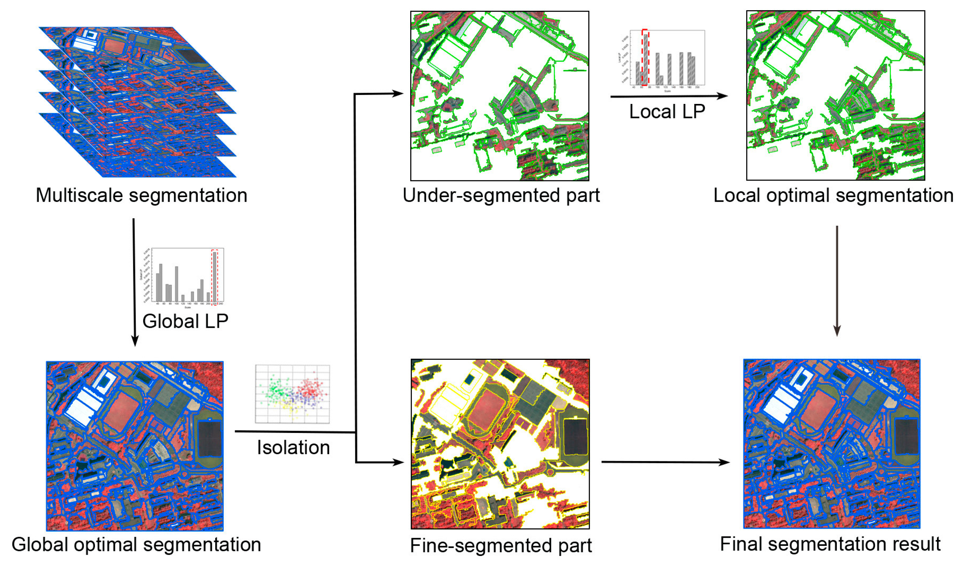
This study proposes a multiscale optimization method for urban green cover segmentation, which aims to comprehensively utilize multiscale segmentation results to achieve optimal scale expression of urban green cover. Figure 1 shows the general framework of the proposed method. First, a global optimal segmentation is selected from the multiscale segmentation results by using an optimization indicator. The indicator is the local peak (LP) of the change rate (CR) of the mean value of spectral standard deviation (SD) of each segment. Second, the regions in the global optimal segmentation result are isolated into under- and fine-segmentation parts, based on designed under-segmentation isolation rule. Third, the under-segmentation regions are refined by using the same optimization indicator LP in a local version. Finally, the fine-segmented part and the optimized under-segmented part are combined to obtain the final cross-scale optimization result.

2.2. Hierarchical Multiscale Segmentation

The hierarchical multiscale segmentation is composed of multiple segments from fine to coarse at each location, in which the small objects are supposed to be represented by fine segments at certain segmentation scales and the large objects are represented by coarse segments correspondingly. Furthermore, a fine-scale segment smaller than a real object is supposed to represent a part of the object, while a coarse-scale segment larger than a real object is to represent an object group. A preliminary requirement for the multiscale segments is that the segments at the same location should be nested. Otherwise the object boundaries would be conflict when combining or fusing the multiscale segments.

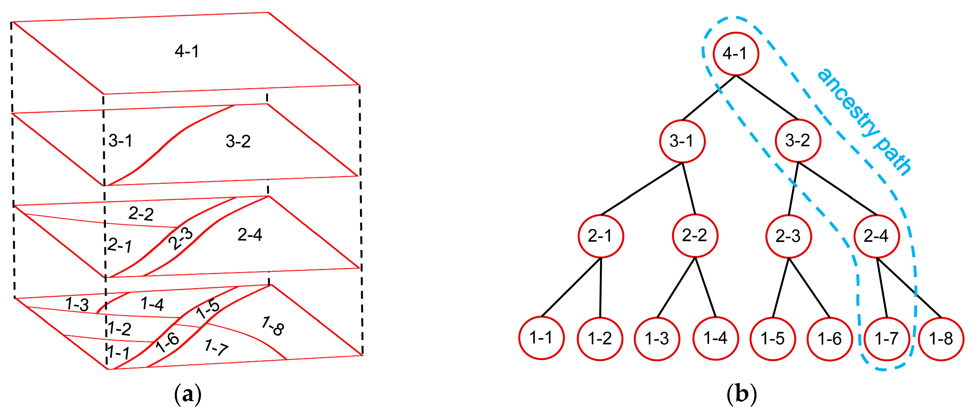
The hierarchical multiscale segmentation is represented using a segment tree model [46], as shown in Figure 2. The tree nodes at different levels represent segments at different scales. An arc connecting a parent and a child node represents the inclusion relation between segments at adjacent scales. The leaf nodes represent the segments at the finest scale and the nodes at upper levels represent segments at coarser scales. Finally, the root node represents the whole image. An ancestry path in the tree is defined as the path from a leaf node up to the root node, revealing the transition from object part to the whole scene. The hierarchical context of each leaf node is conveyed by the ancestry path, in which a segment is gradually becoming coarser and finally reaching the whole image.

Several region-based segmentation methods can be applied to produce the required hierarchical multiscale segmentations, for example multiresolution segmentation method [47], mean-shift method [48] and hierarchical method [49]. Specifically, the multiresolution segmentation method [47] is used in the study, in which the shape parameter is set as 0.5 by default. The regions at each segmentation scale are represented by the nodes at the same level in the segment tree. Finally, the segment tree is constructed by recording the multiscale segmentation.

2.3. Selecting Global Optimal Scale

We need to first select a global optimal segmentation scale and then refine the under-segmentation part for urban green cover. Thus, unlike other optimal scale selection methods for compromising under- and over-segmentation errors, we design an indicator to select an optimal scale in which segmentation results mainly include reasonable under-segmented and fine-segmented regions, reducing over-segmented regions as much as possible.

Referring to the standard deviation indicator [28], we adopt the indicator focusing on homogeneity of segments by calculating the mean value of spectral standard deviation (SD) of each segment. SD is defined as below:

$$SD=\sqrt{\frac{1}{nb}{{\displaystyle \sum }}_{k=1}^b{{\displaystyle \sum }}_{i=1}^{n}S{D}_{ki}}$$

(1)

where SD_ki is the standard deviation of digital number (DN) of spectral band k in segment i; n is the number of segments in the image; and b is the number of spectral bands of the image.

With the increase of the scale parameter, SD will change as following. Generally, it tends to increase because the homogeneity of segments is gradually decreased in the region merging procedure. Near the scale that the segments are close to the real objects, the change rate of SD will increase suddenly because of the influence of the boundary pixels [29].

To find the scale in which the green cover segments are closest to the real objects, we propose indicator CR to represent the change rate of SD and indicator LP to represent the local peak of CR. They are defined respectively as below:

$$CR=\frac{dSD}{dl}=\frac{SD\left(l\right)-SD\left(l-\Delta l\right)}{\Delta l}$$

(2)

$$LP=\left[CR\left(l\right)-CR\left(l-\Delta l\right)\right]+\left[CR\left(l\right)-CR\left(l+\Delta l\right)\right]$$

(3)

where l is the segmentation scale and Δl is the increment in scale parameter, that is the lag at which the scale parameter grows. The scale increment has powerful control over the global optimal segmentation because it can smooth the heterogeneity measure resulting in the optimal segmentation occurred in different scales [50]. Experimentally, the small increments (e.g., 1) produces optimal segmentation in finer scales while the large increments (e.g., 100) produces optimal segmentation in coarser scales [28]. Hence, the medium increment (e.g., 10) of scale is adopted in the study.

According to the aforementioned change law of SD, near the scale that the segments are close to the real objects, the CR will increase suddenly because of the influence of the boundary pixels of green cover segments. Thus, a LP will appear when the global optimal segmentation scale is coming for several segments. However, there are several LPs within a set of increased scale parameters because not all the segments have the same optimal segmentation scale. The global optimal segmentation is identified as the scale with largest LP, because the largest LP indicates that most of the segments in the image reach the optimal segmentation state. Furthermore, the large LP could also be caused by the large SD value of coarse segments, because the large SD will produce large CR and corresponding large LP, revealing the under-segmentation state. Therefore, the next step is to optimize the under-segmentation part of the global optimal segmentation result for green cover objects.

2.4. Isolating Under-Segmented Regions

In order to obtain the under-segmented regions for green cover from the globally optimized segmentation result, further isolation of segments is required. When a green cover object is in the under-segmentation state, it is often mixed with other adjacent objects and the spectral standard deviation (SD_i) is thus great. Moreover, since the normalized difference vegetation index (NDVI) has a good performance to distinguish between green cover and other features, when other objects are mixed with the green cover object, the NDVI value of the region is not very high, that is lower than that of green cover objects, as well as not very low, that is higher than that of non-green cover objects. NDVI is defined as the ratio of difference between near infrared band and red band values to their sum [51]. Thus, NDVI of a region is calculated as below:

$$NDV{I}_i=\frac{1}{m}{{\displaystyle \sum }}_{j=1}^m\frac{NI{R}_j-R_j}{NI{R}_j+R_j}$$

(4)

where NIR_j and R_j are DNs of near infrared and red band for pixel j, respectively; and m is the number of pixels in region i.

Therefore, a region with a high SD_i value and a medium NDVI_i value can be considered an under-segmentation region for green cover. The isolation rule for an under-segmentation region with green cover are thus defined as below:

$$\{\begin{array}{c}S{D}_i>T_{SD}\\ T_{N1}<NDV{I}_i<T_{N2}\end{array}$$

(5)

where T_SD, T_N1, and T_N2 are thresholds that need to be set by users. We set it by the trial-and-error strategy. A segment with SD_i lower than T_SD is viewed as fine segment because of the high homogeneity. If the NDVI_i value of region i is higher than T_N2, it is viewed as fine segmentation of green cover; and if it is lower than T_N1, it is viewed as not containing green cover and will not be involved in the successive refining procedure.

2.5. Refining Under-Segmented Regions

For each individual region in the under-segmentation part, the segment tree is first used to quantify the spatial context relationship of the regions at different scales and the appropriate segmentation scale is then selected through the optimization indicator LP. Finally, the under-segmentation part is replaced by the optimized segments. The specific steps are performed as follows:

(1)

Select one under-segmented region R_i, extract the segmentations at lower scales than the global optimal scale in region R_i.

(2)

Compute the LP of each scale and the local optimal scale of green cover is defined as scale with a largest LP in region R_i.

(3)

Replace R_i with the local optimal scale segmentation.

(4)

Repeat step (1)–(3) until all under-segmented regions are refined according to Equation (5).

2.6. Accuracy Assessment

Segmentation quality evaluation strategies include visual analysis, system-level evaluation, empirical goodness, and empirical discrepancy methods [37]. The last two methods are also known as unsupervised and supervised evaluation methods, respectively. The unsupervised evaluation method calculates indexes of homogeneity within segments and heterogeneity between segments [35]. It does not require ground truth but the explanatory of designing measures and the meaning of measure values is insufficient. The supervised evaluation method compares segmentation results with ground truth and its discrepancy can directly reveal the segmentation quality [52]. Region-based precision and recall measures are sensitive to both geometric and arithmetic errors. Thus, the supervised evaluation method is used to assess the segmentation accuracy of the multiscale optimization.

Precision is the ratio of true positives to the sum of true positives and false positives, and recall is the ratio of true positives to the sum of true positives and false negatives. Given the segmentation result S with n segments {S₁, S₂, …, S_n} and the reference R with m objects {R₁, R₂, …, R_m}, the precision measure is calculated by matching {R_i} to each segment S_i and the recall measure by matching {S_i} to each reference object R_i. When calculating the precision measure, the matched reference object (R_imax) for each segment S_i is first identified, where R_imax has the largest overlapping area with S_i. The precision measure is then defined as [23]:

$$precision=\frac{{{\displaystyle \sum }}_{i=1}^n\left|S_i\cap R_{imax}\right|}{{{\displaystyle \sum }}_{i=1}^n\left|S_i\right|}$$

(6)

where |$·$| denotes the area that is represented by the number of pixels in a region.

Similarly, the matched segment (S_imax) for each reference object R_i is searched according to the maximal overlapping area criterion and the recall measure is defined as [23]:

$$recall=\frac{{{\displaystyle \sum }}_{i=1}^m\left|R_i\cap S_{imax}\right|}{{{\displaystyle \sum }}_{i=1}^m\left|R_i\right|}$$

(7)

The precision and recall measures both range from 0 to 1. Using these two measures can determine both under- and over-segmented situations. An under-segmented result will have a large recall and a low precision. By contrast, if the result is over-segmented, the precision is high but the recall is low. If the precision and recall values of one segmentation result are both higher than another, this result is considered to have a better segmentation quality. However, we do not know which one is better when one measure in larger than another and the other measure is smaller than another. Hence, we should combine these two measures into one. In this study, we use the harmonic average of precision and recall called F-score [53], which is defined as:

$$\mathit{F-score}=\frac{2·precsion·recall}{precsion+recall}$$

(8)

where an F-score reaches its best value at 1 (perfect precision and recall) and worst at 0.

3. Data

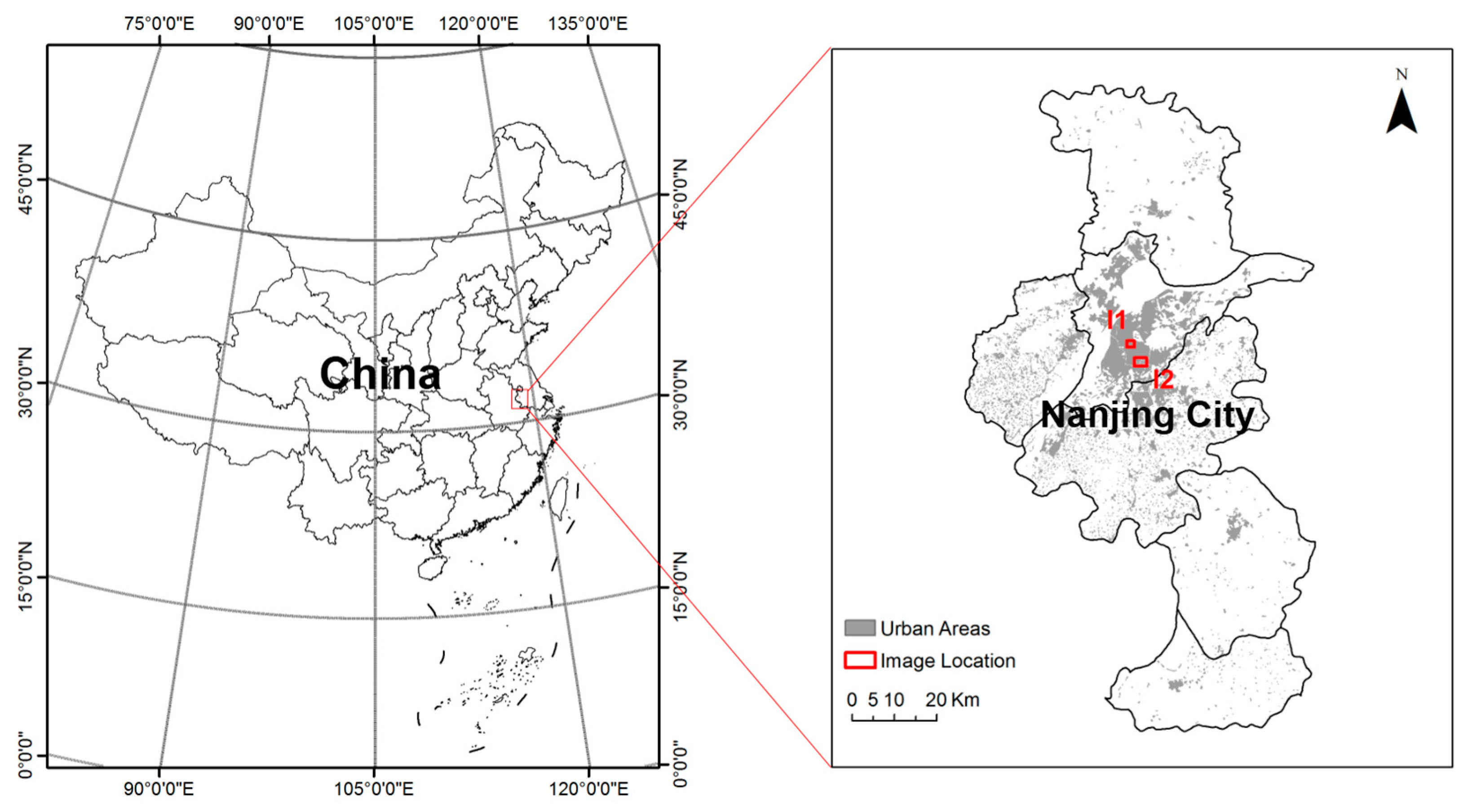
The study area is located in Nanjing City (32°02′38″N, 118°46′43″E), which is the capital of Jiangsu Province of China and the second largest city in the East China region (Figure 3), with an administrative area of 6587 km² and a total population of 8335 thousand as of 2017. As one of the four garden cities in China, Nanjing has a wealth of urban green spaces than many of other cities. The urban green cover rate in the built-up area of Nanjing is 44.85% in 2018.

In this study, an IKONOS-2 image acquired on 19 October 2010 and a WorldView-2 image acquired on 29 July 2015 in Nanjing are used as the HR data. Both the images consist of four spectral bands: blue, green, red, and near infrared. The spatial resolution of the multispectral bands of the IKONOS-2 image is improved from 3.2 m to 0.8 m after pan-sharpening. The spatial resolution of the multispectral bands of the WorldView-2 image is 2 m.

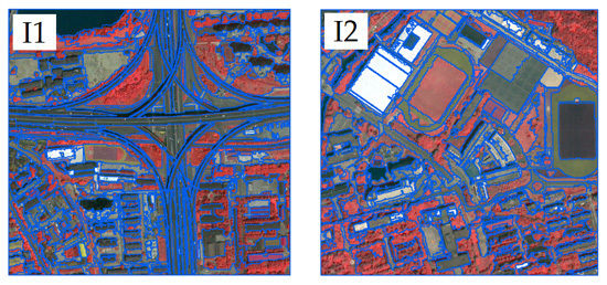
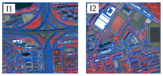
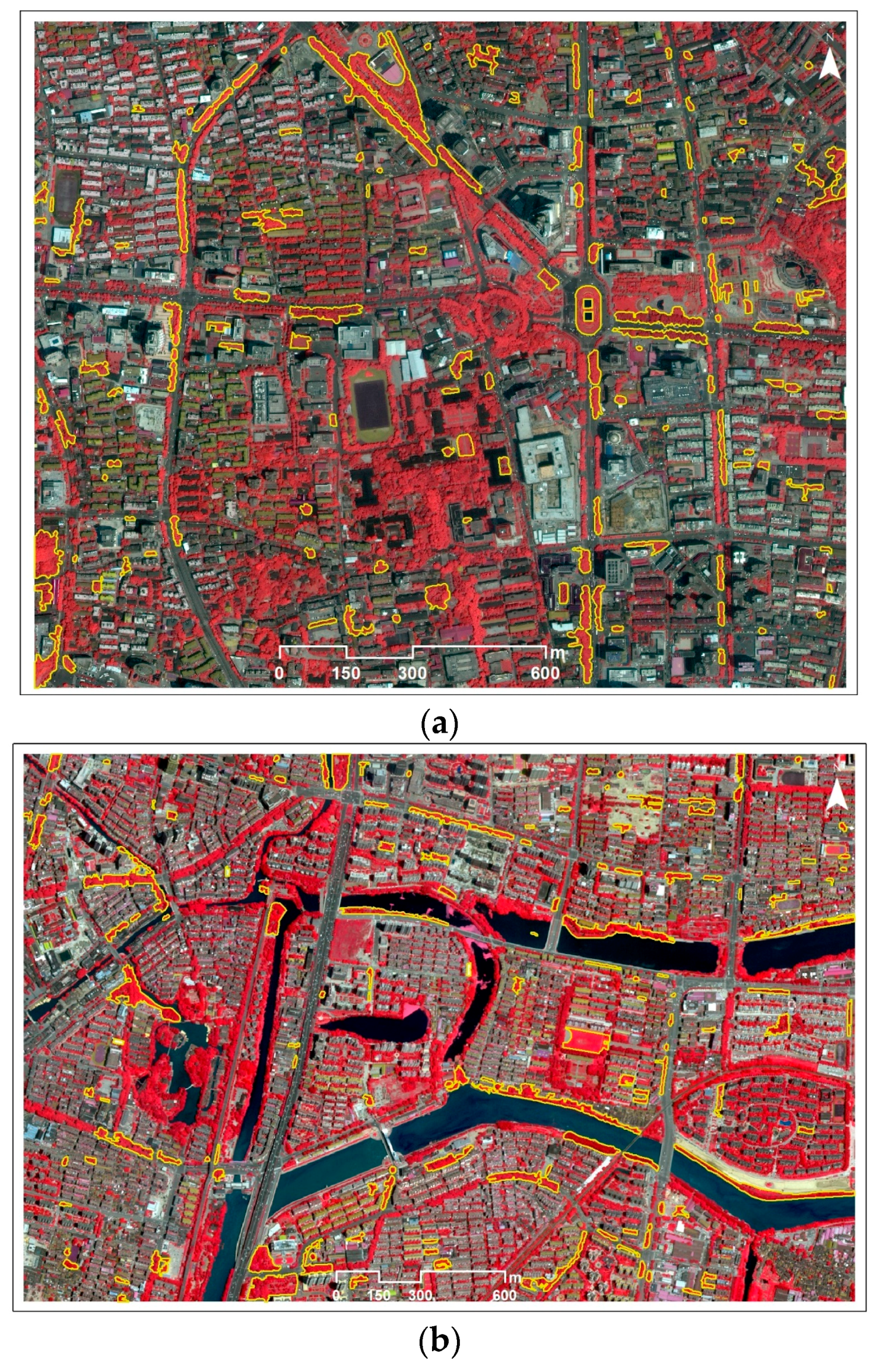
Two test images identified as I1 and I2 are subsets of the IKONOS-2 and the WorldView-2 images, respectively, containing urban green cover in traffic area, residential area, campus area, park area, commercial area, and industrial area, which are the typical areas in urban. The size of I1 and I2 are 2286 × 1880 and 1478 × 974 pixels and the area are approximate 2.8 km² and 5.8 km², respectively. As shown in Figure 4, there are abundant green cover objects distributed in the images and various in size and shape.

In order to evaluate the segmentation accuracy, we randomly select some green cover objects as reference. The reference objects are uniformly distributed in the test images and various in size and shape. Each reference object is delineated by one person and reviewed by other to catch any obvious errors. Finally, we collect 130 reference objects for each test image. It is noted that if there are trees covered a road, this area will be digitized as green cover objects. The area of the smallest reference object is only 59.5 m², whereas the area of the biggest reference object is 14,063.1 m². Hence, it is not possible to properly segment all of the green cover objects using a single segmentation scale.

4. Results

4.1. Global Optimal Scale Selection

The multiscale segmentation results are produced by applying multiresolution segmentation method. For I1, the scale parameters are set from 10 to 250 by increment of 10. Since the spatial resolution of I2 is coarser than I1, the scale parameters are set from 10 to 125 by increment of 5. If we set the same scale parameters for I2 as those for I1, the coarse segmentation scales (e.g., >130) would be seriously under-segmented and the homogeneity of segments at these coarse scales would change randomly, which could not benefit the optimization procedure and could even do harm to the optimization procedure.

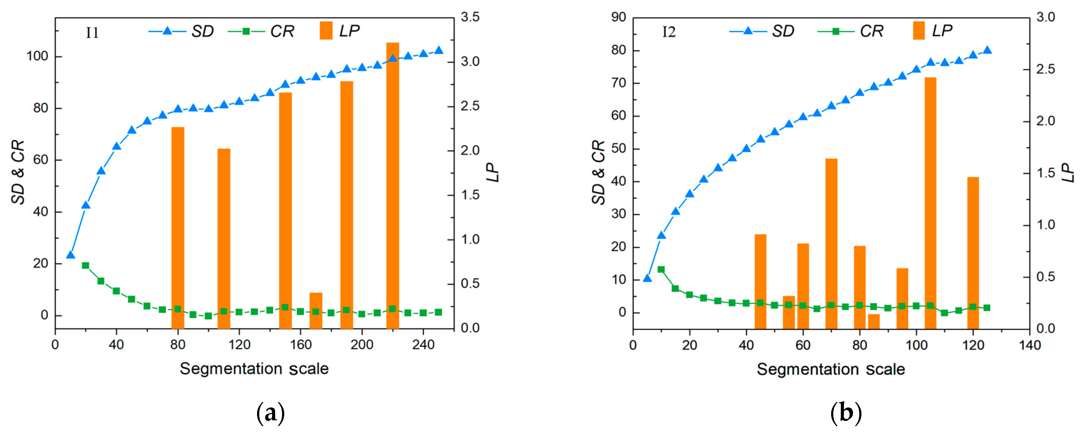
The multiscale segmentations cover apparently over-segmentation, medium segmentation, and apparently under-segmentation. The optimization indicators SD, CR, and LP are respectively calculated for each segmentation result and shown in Figure 5. When the scale parameter increases, SD gradually increases, which indicates that the regions are gradually growing and the homogeneity decreases. Correspondingly, in the process of SD change, CR appears multiple local peaks. The indicator LP can highlight these local peaks of CR very well. We can see that LP appears at segmentation scales of 80, 110, 150, 170, 190, and 220 for I1, in which LP reaches the maximum at 220. For I2, LP appears at segmentation scales of 45, 55, 60, 70, 80, 85, 95, 105, and 120, where LP is the largest at 105. Therefore, the segmentation with the scale parameter of 220 and 105 is taken as the global optimal segmentation scale for I1 and I2.

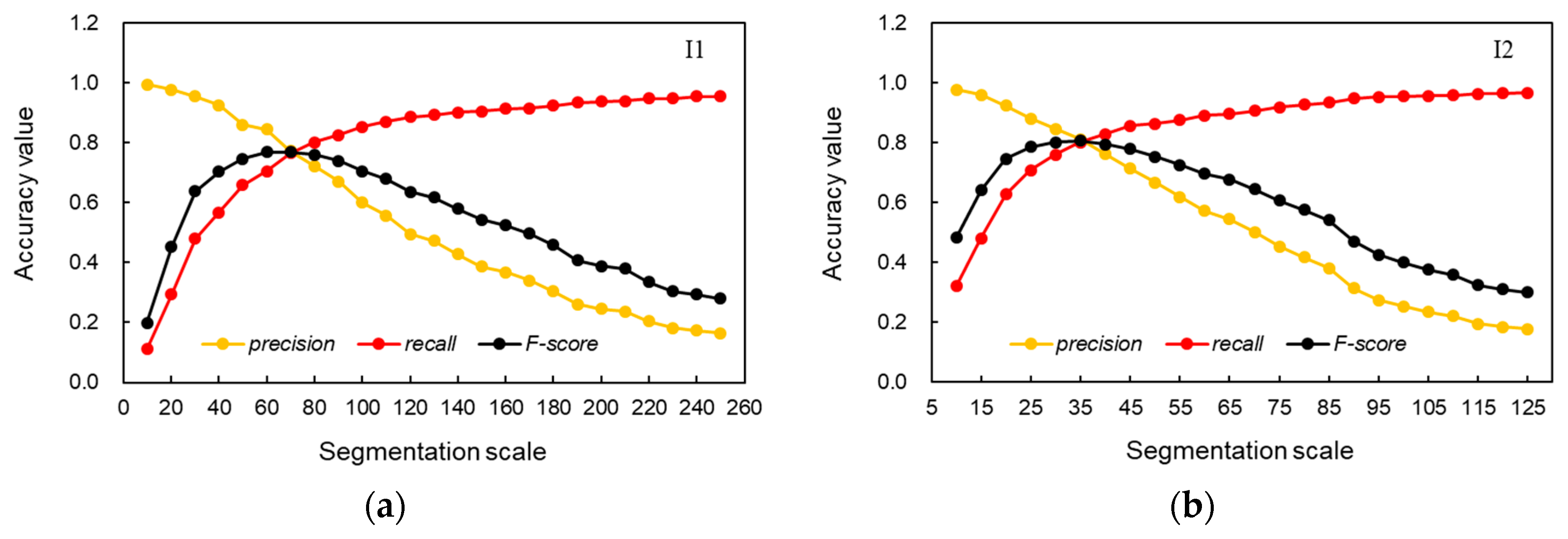
Combining with the supervised evaluation results of the multiscale segmentations (Figure 6), we can know that the selected global optimal segmentation scale is at the under-segmentation status for green cover objects. For both I1 and I2, the precision value is apparently lower than the recall value in the optimal scale, which indicates the under-segmentation status. 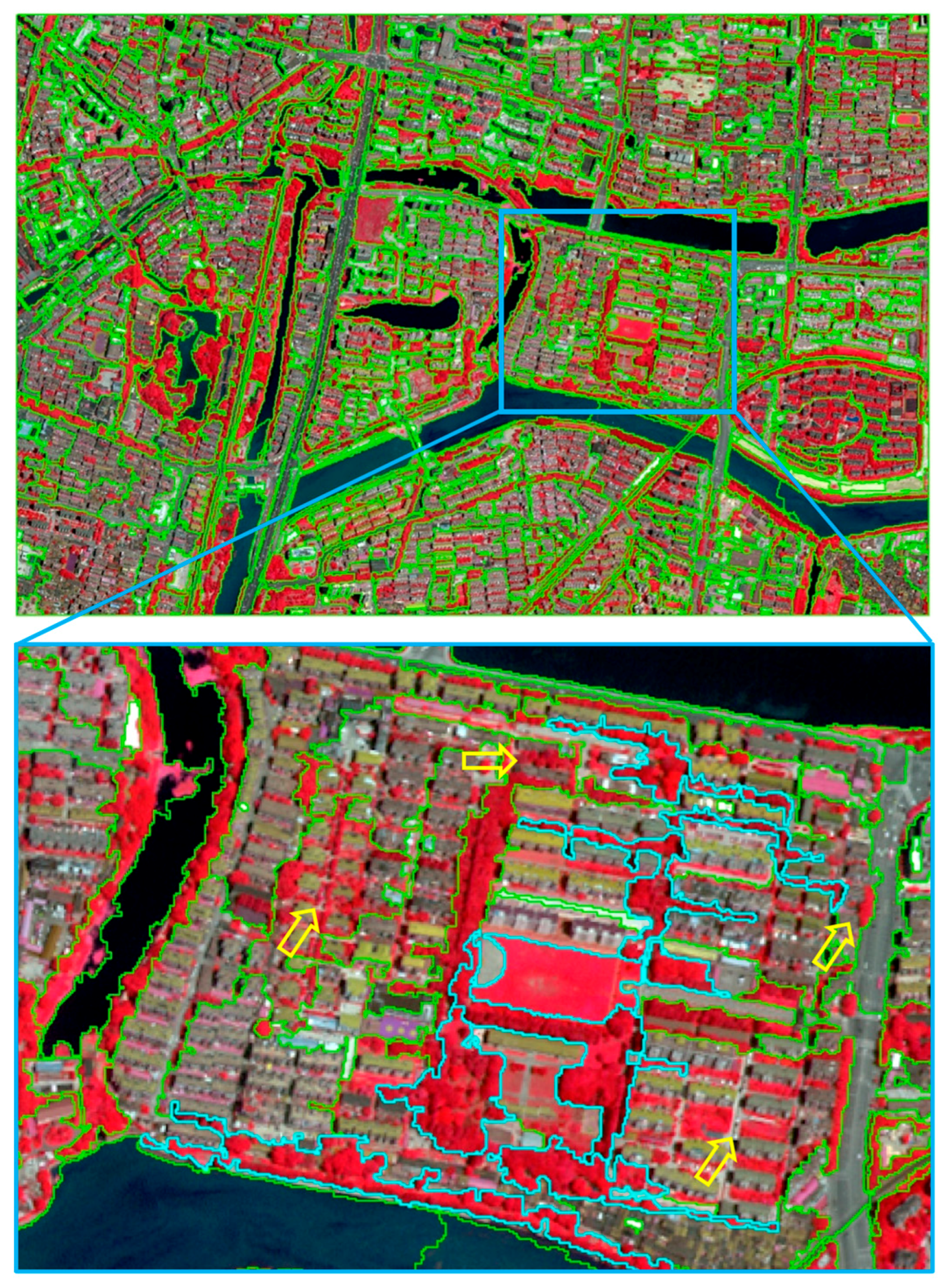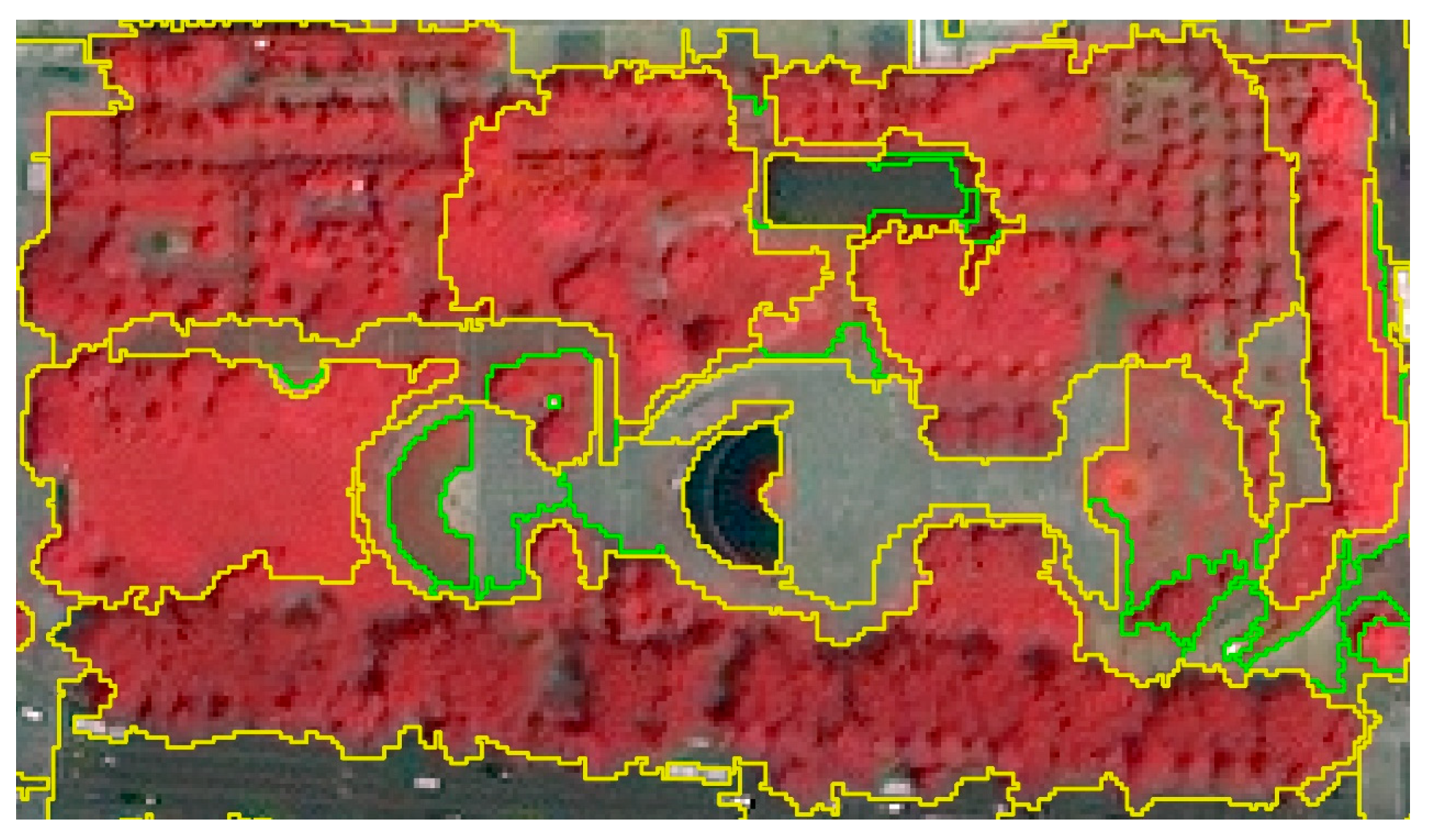To further illustrate this, the selected I2 segmentation result at scale 105 is presented in Figure 7, in which we can clearly see that except for several fine-segmented green cover objects with relatively large size, many green cover objects are shown as under-segmented.

The selected global optimal segmentation of green cover tends to appear in the case of coarse scales. As a result, the over-segmentation errors are reduced, while some green cover objects with small size will inevitably be in an under-segmentation state and single scale cannot achieve optimal segmentation of green cover objects of different sizes. Therefore, it is necessary to further optimize the global optimal segmentation by refining the under-segmented regions.

4.2. Under-Segmented Region Isolation

The under-segmented regions are isolated by the rule in Equation (5). The threshold values of T_SD, T_N1, and T_N2 are set as 40, 0.05, and 0.25 for test image I1 and as 40, 0.10, and 0.55 for test image I2. The threshold values of NDVI_i for I2 is set as different for I1, this is mainly because the different acquisition date between I1 and I2, between which the vegetation growth status is different.

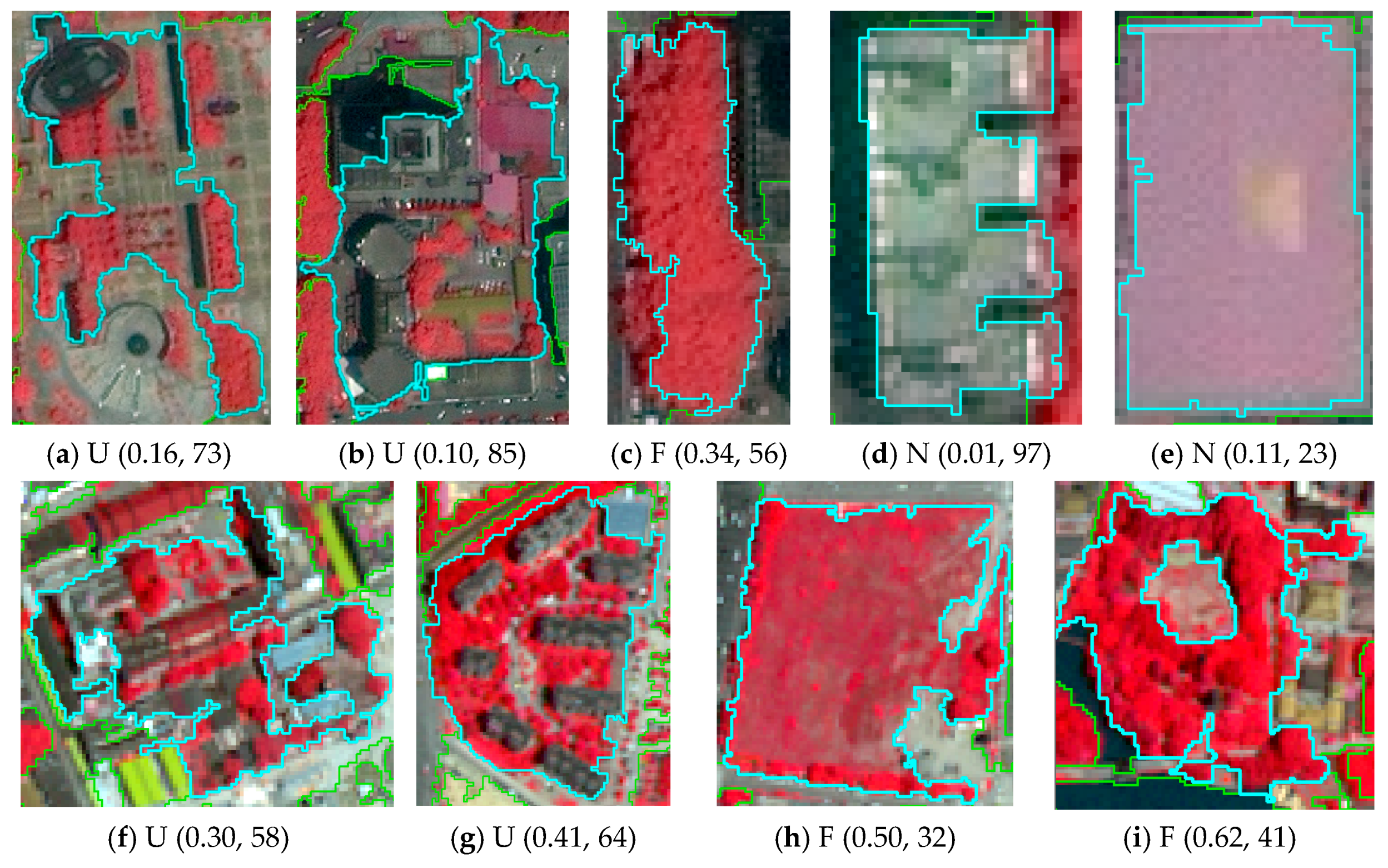
To illustrate the effectiveness of the designed isolation rule for under-segmentation with green cover, several sample segments in the global optimal segmentations are presented in Figure 8. It can be seen that the under-segmented regions containing green cover have medium NDVI_i values and high SD_i values, as shown in Figure 8a,b,f,g. The fine-segmentation of green cover present high NDVI_i values as shown in Figure 8c,i. A special case of fine-segmentation is shown in Figure 8h, which is a segment mainly containing sparse grass and the NDVI_i value is thus not very high. However, the relatively low SD_i value of grass segment can prevent it to be wrongly identified as under-segmentation. The segments without green cover usually present low NDVI_i value as shown in Figure 8d. A special case of segment without green cover is shown in Figure 8e, where the roof segment has a medium NDVI_i value because of the roof material. However, the relatively low SD_i value can prevent it to be wrongly identified as under-segmentation containing green cover.

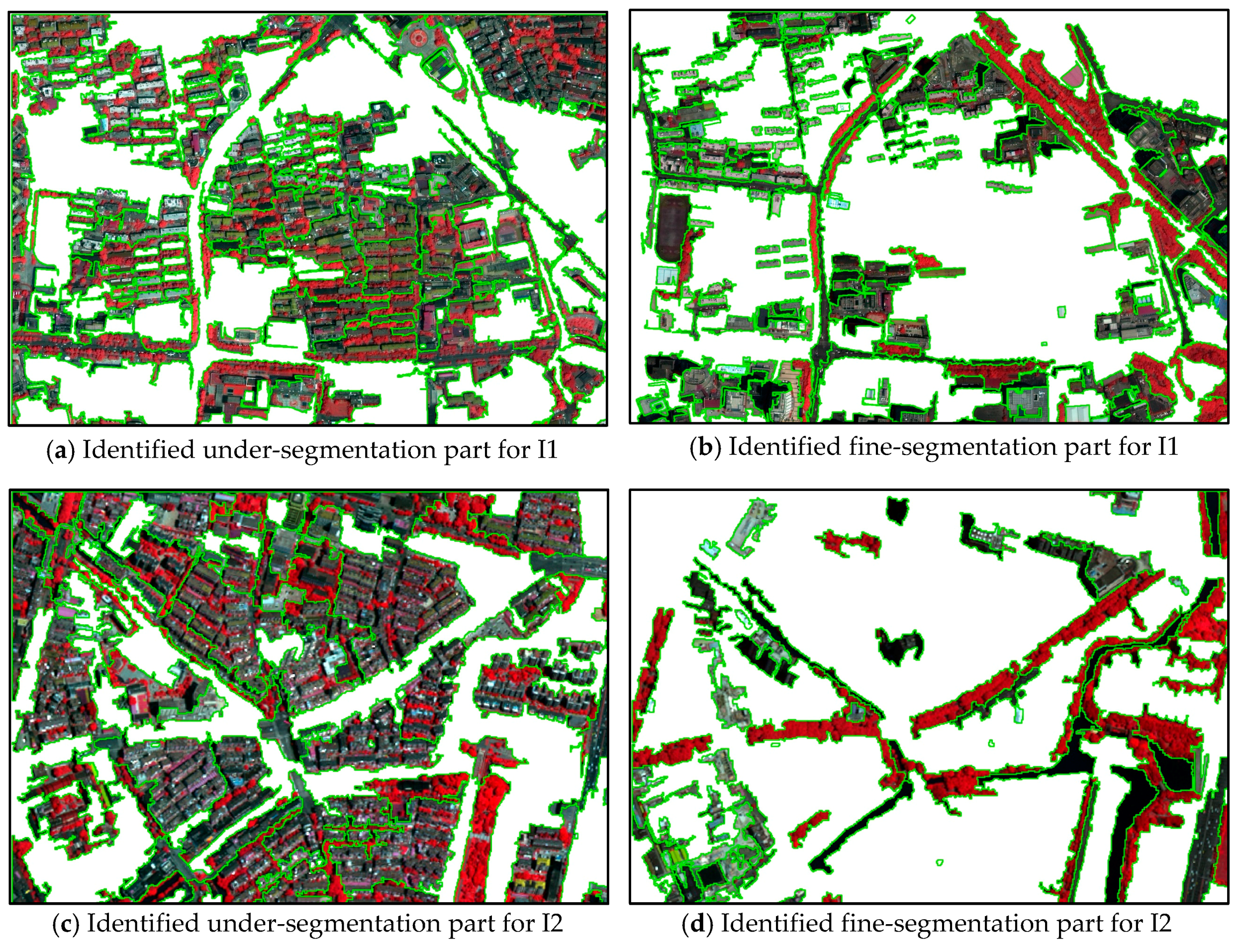
To further validate the effectiveness of the isolation rule, the up-left part of the isolation results of I1 and I2 is zoomed in Figure 9. It can be seen that the green cover and other objects are mixed in the isolated under-segmented regions. In the fine-segmentation part, the regions are either fine-segmented green cover or segments without green cover.

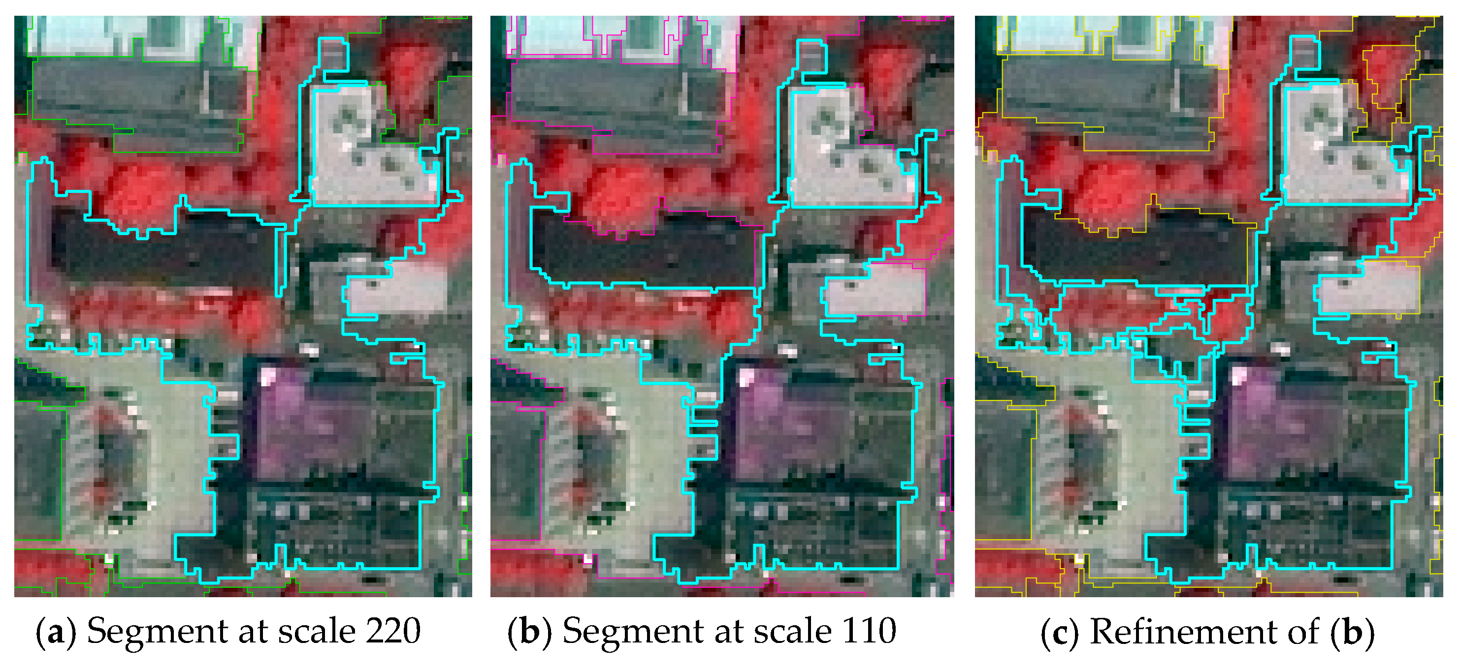
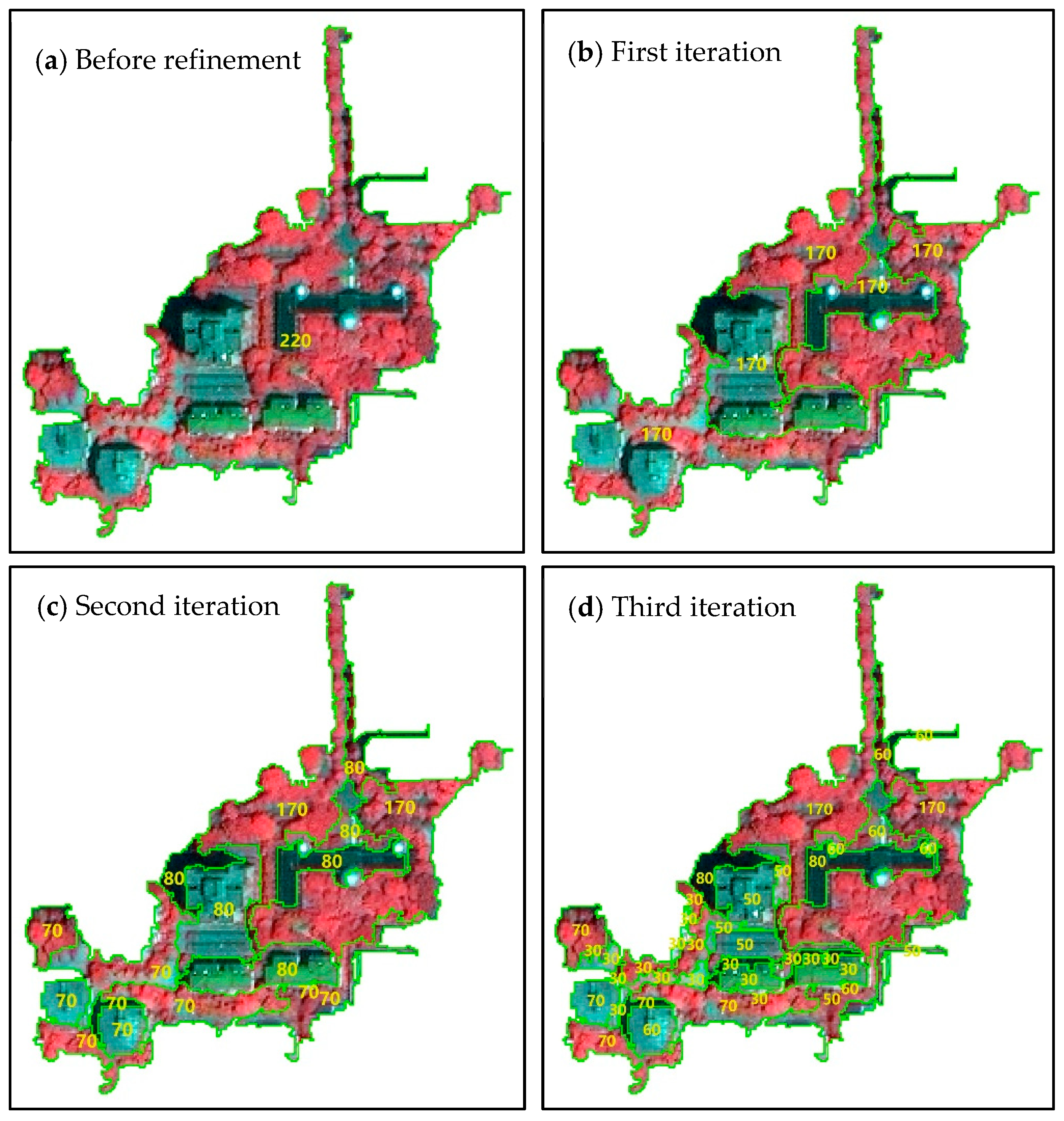
4.3. Under-Segmented Region Refinement

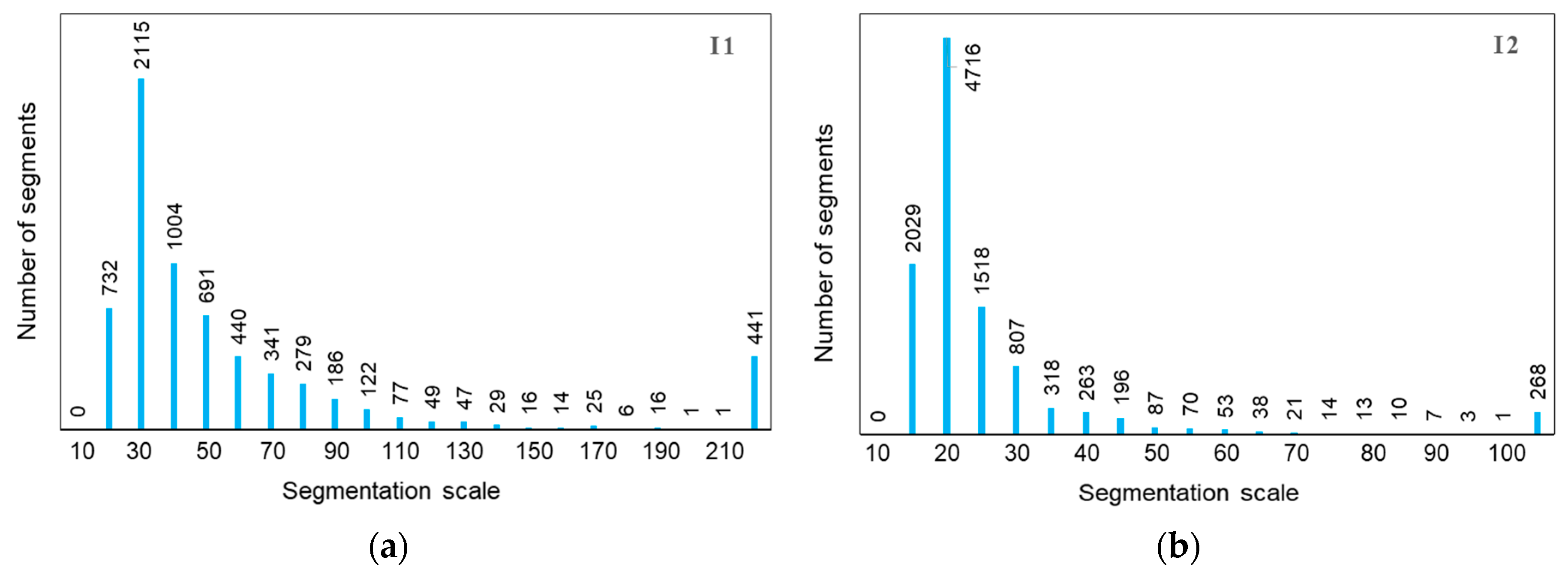
The multiscale optimized segmentation is obtained by refining the under-segmented part of the global optimal scale. In the refinement segmentation result, with the benefit of cross-scale refinement strategy, the segments are at different segmentation scales to achieve the optimal segmentation scale for each green cover object. The histogram of segmentation scales in the refinement results is shown in Figure 10. The refined segments almost cover all the segmentation scales finer than the selected global optimal scale. There are many segments at the small segmentation scales, for example scale 20 to 40 for I1 and scale 15 to 25 for I2, because there are many small-size green cover objects in urban area, such as single trees.

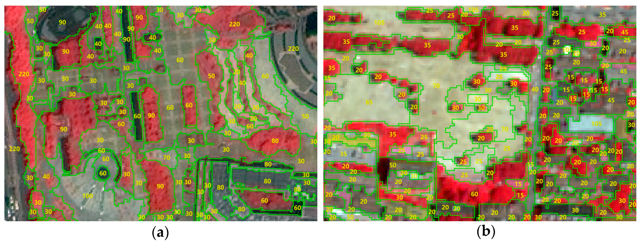
To illustrate the effectiveness of achieving optimal scale for each green cover object, the sample refinement results from test images are enlarged to present in Figure 11 with labels of the scale number for each segment. Generally, it can be seen that large green cover objects are segmented at relatively coarse segmentation scales while small green cover objects are segmented at relatively small segmentation scales. The green cover objects, especially the small ones, tend to be segmented by a single segment.

The supervised evaluation results of segmentation before and after refinement are presented in

Table 1. Comparisons of the segmentation accuracy for the result before refinement, after refinement, and the single-scale best result.

	I1			I2
	precision	recall	F-score	precision	recall	F-score
Before refinement	0.204	0.948	0.336	0.234	0.955	0.376
After refinement	0.764	0.811	0.787	0.766	0.859	0.810
Single-scale best	0.773	0.766	0.770	0.812	0.801	0.806

to quantify the effectiveness of the under-segmentation refinement. It can be seen that the precision value is apparently improved after refinement, showing that the under-segmented green cover objects can be effectively refined. The recall value is decreased mainly because the reduced under-segmentation. Therefore, the F-score after refinement is apparent improved than that before refinement. The segmentation results before and after refinement shown in Figure 12 further prove this.

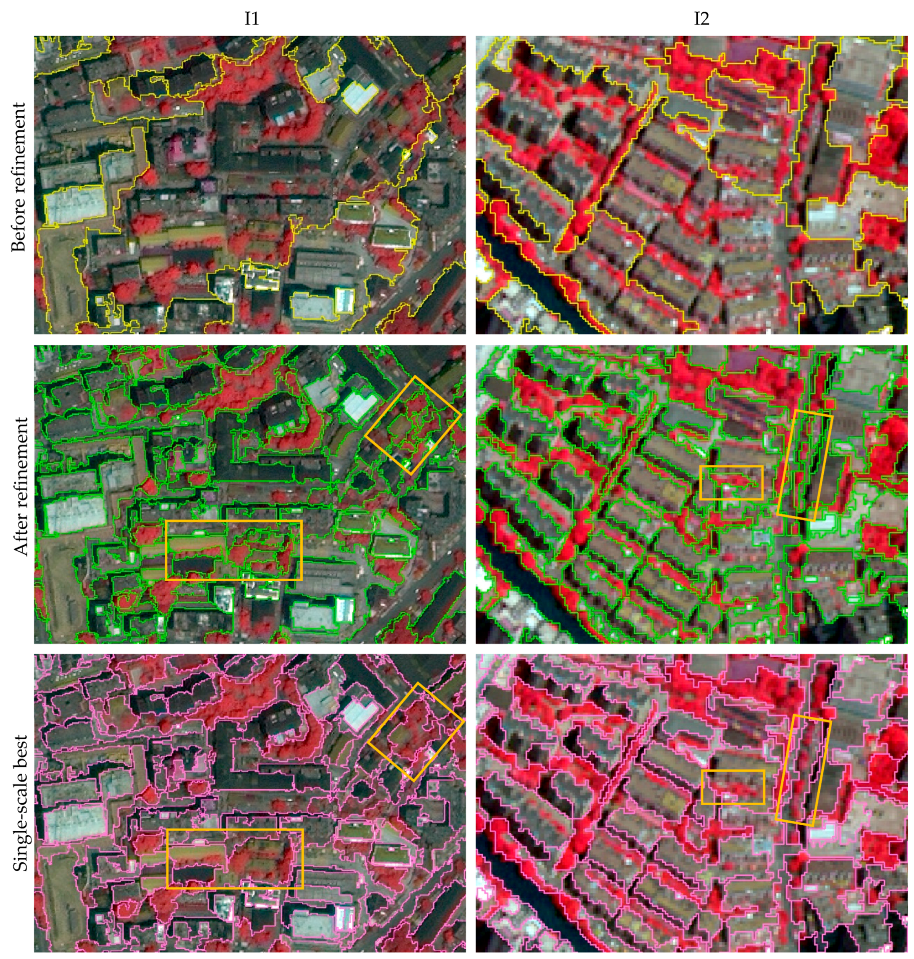
To quantify the effectiveness of cross-scale optimization, the refinement result is compared with single-scale segmentation that has the highest F-score in the produced multiscale segmentations, which is at scale 70 for I1 and 35 for I2. The supervised evaluation results are also presented in Table 1. It can be seen that the precision of the refinement result is slightly lower than that of the single-scale best result while the recall is higher, which could be caused by the over-segmentation of the large green cover objects. Another reason for the lower precision for the refinement result could be caused by the wrong identification of under-segmented green cover objects, which makes the under-segmentation cannot be refined and thus lowers the precision accuracy. As a whole, the F-score of the refinement result is slightly higher than that of the single-scale best segmentation, which could mainly be caused by the reduced under-segmentation errors in the refining procedure. The segmentation results presented in Figure 11 further show the difference. As highlighted by the yellow rectangles, the existed under-segmentation errors in the single-scale best segmentation can be effectively reduced by the proposed refining strategy, which indicates the effectiveness of the refining procedure on overcoming under-segmentation errors. According to the comparison result with single-scale best segmentation, we can safely conclude that the proposed unsupervised multiscale optimization method can automatically produce optimal segmentation result at least equals to single-scale best segmentation indicated by supervised evaluation. Furthermore, the proposed refining strategy can help to reduce under-segmentation errors even in the single-scale best segmentation.

5. Discussions

5.1. Influence of Selected Global Optimal Segmentation Scale

The selected global segmentation scale is assumed to be reasonably under-segmented, which means that a part of segments is under-segmented and others are fine-segmented with few over-segmentation errors. This is because the successive refining procedure is designed to reduce the under-segmentation errors rather than over-segmentation errors. The results in Section 4.1 proved that the used optimization indicator can select segmentation scale at under-segmentation status. However, we can see from Figure 7 that many segments in the selected segmentation are extensively under-segmented, especially for those containing small green cover objects. Actually, the extensive under-segmentation could make the refinement difficult because too many different objects are mixed, which makes the segment features become erratic or random.

Even though the automatically selected global optimal segmentation scale can result in satisfactory refinement result, we explored whether a less under-segmentation than the selected one could further improve the refinement performance. For test images I1 and I2, a less under-segmented scale than the automatically selected one is input to the refining procedure and the segmentation accuracies of the refinement results are presented in

Table 2. Comparisons of the segmentation accuracy for the refinement results from different global segmentation scale.

	I1				I2
Global Scale	precision	recall	F-score	Global Scale	precision	recall	F-score
220	0.764	0.811	0.787	105	0.766	0.859	0.810
110	0.826	0.788	0.807	70	0.791	0.846	0.817

. It is noted that the less under-segmented scale is also a local peak in Figure 5. We can see that the less under-segmented global segmentation scale could result in higher precision and higher F-score accuracies, which is because the prevalent under-segmentation is reduced that achieves better refinement performance. The sample segments of I1 shown in Figure 13 illustrate the difference. The segment at scale 220 in Figure 13a is prevalent under-segmented in terms of the green cover object, the NDVI_i value of which is thus very low and it is not identified as the under-segmentation by the rule. Therefore, it is not involved in the following refinement procedure and the under-segmentation error is presented in the refinement result. However, the corresponded segment at scale 110 is less under-segmented and the NDVI_i value is higher than that at scale 220, which make it allowed to be refined to remove the under-segmentation error. As a whole, this example demonstrates the importance of selecting a reasonable under-segmentation scale for the successive refinement. Specifically, the segments should better not be prevalent under-segmented.

5.2. Key Role of Identifying Under-Segmented Region

Based on the global segmentation scale with under-segmentation, the identification of under-segmented region serves as a key role to reduce under-segmentation errors once the refinement procedure is effective. Hence, before illustrating the key role of identifying under-segmented region, the effectiveness of refinement procedure is further judged in addition to Section 4.3.

Since the optimization indicator of maximum LP tends to select under-segmented scale, it makes the refining procedure performed iteratively because the selected optimal scale in the refining procedure could still be under-segmented for some segments and these segments need to be further refined. This increases the calculations for the refinement but it can lead to the safe refinement that avoids new over-segmentation errors.

The segmentation accuracies in the refining procedure of image I1 are presented in

Table 3. Segmentation accuracies in the refining procedure of I1.

	precision	recall	F-score
Before refinement	0.204	0.948	0.336
First iteration	0.492	0.899	0.636
Second iteration	0.693	0.835	0.757
Third iteration	0.764	0.811	0.787

, through which we can see that the F-score is gradually increased. This is caused by the iteratively reduced under-segmentation errors in the refining procedure, which shows the effectiveness of the refining strategy and also the effectiveness of the isolation rule for under-segmented region. The sample segments in Figure 14 further demonstrates the effectiveness of the refining procedure.

As discussed above, the identification of under-segmented region serves as a key role in the proposed method. If the under-segmented regions can be correctly identified, the refinement can achieve success on removing under-segmentation errors because the refining procedure stops when the segment is not identified as under-segmented. Furthermore, if the under-segmented regions cannot be correctly identified, it cannot even be involved into the refining procedure and the under-segmentation error would be preserved in the refinement result. The proposed isolation rules of this study is still primary, which need to set appropriate thresholds by users. Even though it is proved to be effective, the automatic isolation of under-segmentation is still needed to be explored in the future.

5.3. Potential of Segmenting Different Types of Urban Green Cover

The proposed cross-scale optimization method aims at segment urban green cover into single regions by reducing both the under- and over-segmentation errors. The segmentation of urban green cover in general can be practically used in urban planning, for example investigation of urban green cover rate [42,43], and urban environment monitoring, for example influence analysis of the urban green cover to residential quality [44,45]. Surely, it would be more practical useful to segment different types of urban green cover [3,12]. To achieve this by the proposed method, the key step is to adjust isolation rule to identify the under-segmented regions containing different types of green cover. Since the optimization indicator used in the global segmentation scale selection and local refinement is based on the spectral standard deviation, it should be able to deal with under-segmentation for different green cover types. Once the under-segmentation for different types of green cover can be identified, the refining procedure is expected to be able to reduce the corresponding under-segmentation error and separate different types of green cover.

Actually, even though the presented method is not aiming at segmenting different types of green cover, several under-segmented segments containing different types of green cover are refined into each type when they meet the isolation rule in this study. An example of isolating different types of green cover based on scale 110 for image I1 is shown in Figure 15. This shows the potential of adjusting the under-segmentation isolating rule to achieve separating different types of green cover in the future.

5.4. Potential of Refining Under-Segmented Regions for Other Land Cover Types

The under-segmented segments for urban green cover contain other land cover types, for example buildings, roads, and water. These segments are also under-segmented for the non-green-cover objects in it. When refining the under-segmentation for green cover, the under-segmentation errors for other land cover objects are also refined, as shown in Figure 11, Figure 12, Figure 13, Figure 14 and Figure 15. That is to say, the non-green-cover objects in the identified under-segmented segments could also be refined along with the refinement of green cover objects. This reveals the potential of refining other land cover objects by applying the proposed optimization method.

As discussed above, the optimization indicator used in the global segmentation scale selection and local refinement should be able to deal with under-segmentation for different land cover types because it is based on the spectral standard deviation. Accordingly, if a proper isolation rule for other land cover types is designed, the proposed method is expected to be able to optimize the segmentations for those objects, which is also a direction of the future work based on this study.

6. Conclusions

In this paper, a multiscale optimized segmentation method for urban green cover is proposed. The global optimal segmentation result is first selected from the hierarchical multiscale segmentation results by using the optimization indicator global LP. Based on this, under-segmented regions and fine-segmented regions are isolated by the designed rule. For under-segmented regions, local LP is used for refinement, which ultimately allows urban green cover objects of different sizes to be expressed at their optimal scale.

The effectiveness of proposed cross-scale optimization method is proved by experiments based on two test HR images in Nanjing, China. With the benefit of cross-scale optimization, the proposed unsupervised multiscale optimization method can automatically produce optimal segmentation result with higher segmentation accuracy than single-scale best segmentation indicated by supervised evaluation. Furthermore, the proposed refining strategy is demonstrated to be able to effectively reduce under-segmentation errors.

The proposed method can be improved and extended in the future, for example optimizing segmentation for different types of urban green cover or even other land cover types. The key step is to design appropriate isolation rule of under-segmentation for specific applications. To further explore the potentials of the proposed method would be the main future work based on this study.

References

1. Kanniah, K.D. Quantifying green cover change for sustainable urban planning: A case of Kuala Lumpur, Malaysia. Urban For. Urban Green. 2017, 27, 287–304. [Google Scholar] [CrossRef]
2. Salbitano, F.; Borelli, S.; Conigliaro, M.; Chen, Y. Guidelines on Urban and Peri-Urban Forestry; FAO Forestry Paper (FAO); FAO: Rome, Italy, 2016; ISBN 978-92-5-109442-6. [Google Scholar]
3. Wen, D.; Huang, X.; Liu, H.; Liao, W.; Zhang, L. Semantic Classification of Urban Trees Using Very High Resolution Satellite Imagery. IEEE J. Sel. Top. Appl. Earth Obs. Remote Sens. 2017, 10, 1413–1424. [Google Scholar] [CrossRef]
4. Nichol, J.; Lee, C.M. Urban vegetation monitoring in Hong Kong using high resolution multispectral images. Int. J. Remote Sens. 2005, 26, 903–918. [Google Scholar] [CrossRef]
5. Iovan, C.; Boldo, D.; Cord, M. Detection, Characterization, and Modeling Vegetation in Urban Areas from High-Resolution Aerial Imagery. IEEE J. Sel. Top. Appl. Earth Obs. Remote Sens. 2008, 1, 206–213. [Google Scholar] [CrossRef]
6. Ouma, Y.O.; Tateishi, R. Urban-trees extraction from Quickbird imagery using multiscale spectex-filtering and non-parametric classification. ISPRS J. Photogramm. Remote Sens. 2008, 63, 333–351. [Google Scholar] [CrossRef]
7. Tooke, T.R.; Coops, N.C.; Goodwin, N.R.; Voogt, J.A. Extracting urban vegetation characteristics using spectral mixture analysis and decision tree classifications. Remote Sens. Environ. 2009, 113, 398–407. [Google Scholar] [CrossRef]
8. Huang, X.; Lu, Q.; Zhang, L. A multi-index learning approach for classification of high-resolution remotely sensed images over urban areas. ISPRS J. Photogramm. Remote Sens. 2014, 90, 36–48. [Google Scholar] [CrossRef]
9. Blaschke, T.; Hay, G.J.; Kelly, M.; Lang, S.; Hofmann, P.; Addink, E.; Queiroz Feitosa, R.; van der Meer, F.; van der Werff, H.; van Coillie, F.; et al. Geographic Object-Based Image Analysis—Towards a new paradigm. ISPRS J. Photogramm. Remote Sens. 2014, 87, 180–191. [Google Scholar] [CrossRef] [PubMed]
10. Ardila, J.P.; Bijker, W.; Tolpekin, V.A.; Stein, A. Context-sensitive extraction of tree crown objects in urban areas using VHR satellite images. Int. J. Appl. Earth Obs. Geoinf. 2012, 15, 57–69. [Google Scholar] [CrossRef] [Green Version]
11. Yin, W.; Yang, J. Sub-pixel vs. super-pixel-based greenspace mapping along the urban–rural gradient using high spatial resolution Gaofen-2 satellite imagery: A case study of Haidian District, Beijing, China. Int. J. Remote Sens. 2017, 38, 6386–6406. [Google Scholar] [CrossRef]
12. Puissant, A.; Rougier, S.; Stumpf, A. Object-oriented mapping of urban trees using Random Forest classifiers. Int. J. Appl. Earth Obs. Geoinf. 2014, 26, 235–245. [Google Scholar] [CrossRef]
13. Dey, V.; Zhang, Y.; Zhong, M. A review on image segmentation techniques with remote sensing perspective. In Proceedings of the ISPRS TC VII Symposium—100 Years ISPRS, Vienna, Austria, 5–7 July 2010; Volume XXXVIII. Part 7A. [Google Scholar]
14. Mathieu, R.; Freeman, C.; Aryal, J. Mapping private gardens in urban areas using object-oriented techniques and very high-resolution satellite imagery. Landsc. Urban Plan. 2007, 81, 179–192. [Google Scholar] [CrossRef]
15. Moskal, L.M.; Styers, D.M.; Halabisky, M. Monitoring Urban Tree Cover Using Object-Based Image Analysis and Public Domain Remotely Sensed Data. Remote Sens. 2011, 3, 2243–2262. [Google Scholar] [CrossRef] [Green Version]
16. Benz, U.C.; Hofmann, P.; Willhauck, G.; Lingenfelder, I.; Heynen, M. Multi-resolution, object-oriented fuzzy analysis of remote sensing data for GIS-ready information. ISPRS J. Photogramm. Remote Sens. 2004, 58, 239–258. [Google Scholar] [CrossRef] [Green Version]
17. Blaschke, T. Object based image analysis for remote sensing. ISPRS J. Photogramm. Remote Sens. 2010, 65, 2–16. [Google Scholar] [CrossRef]
18. Kim, M.; Warner, T.A.; Madden, M.; Atkinson, D.S. Multi-scale GEOBIA with very high spatial resolution digital aerial imagery: Scale, texture and image objects. Int. J. Remote Sens. 2011, 32, 2825–2850. [Google Scholar] [CrossRef]
19. Carleer, A.P.; Debeir, O.; Wolff, E. Assessment of Very High Spatial Resolution Satellite Image Segmentations. Photogramm. Eng. Remote Sens. 2005, 71, 1285–1294. [Google Scholar] [CrossRef]
20. Tian, J.; Chen, D.-M. Optimization in multi-scale segmentation of high-resolution satellite images for artificial feature recognition. Int. J. Remote Sens. 2007, 28, 4625–4644. [Google Scholar] [CrossRef]
21. Liu, Y.; Bian, L.; Meng, Y.; Wang, H.; Zhang, S.; Yang, Y.; Shao, X.; Wang, B. Discrepancy measures for selecting optimal combination of parameter values in object-based image analysis. ISPRS J. Photogramm. Remote Sens. 2012, 68, 144–156. [Google Scholar] [CrossRef]
22. Witharana, C.; Civco, D.L.; Meyer, T.H. Evaluation of data fusion and image segmentation in earth observation based rapid mapping workflows. ISPRS J. Photogramm. Remote Sens. 2014, 87, 1–18. [Google Scholar] [CrossRef]
23. Zhang, X.; Feng, X.; Xiao, P.; He, G.; Zhu, L. Segmentation quality evaluation using region-based precision and recall measures for remote sensing images. ISPRS J. Photogramm. Remote Sens. 2015, 102, 73–84. [Google Scholar] [CrossRef]
24. Witharana, C.; Civco, D.L. Optimizing multi-resolution segmentation scale using empirical methods: Exploring the sensitivity of the supervised discrepancy measure Euclidean distance 2 (ED2). ISPRS J. Photogramm. Remote Sens. 2014, 87, 108–121. [Google Scholar] [CrossRef]
25. Cardoso, J.S.; Corte-Real, L. Toward a generic evaluation of image segmentation. IEEE Trans. Image Process. 2005, 14, 1773–1782. [Google Scholar] [CrossRef] [PubMed] [Green Version]
26. Espindola, G.M.; Camara, G.; Reis, I.A.; Bins, L.S.; Monteiro, A.M. Parameter selection for region-growing image segmentation algorithms using spatial autocorrelation. Int. J. Remote Sens. 2006, 27, 3035–3040. [Google Scholar] [CrossRef]
27. Drǎguţ, L.; Tiede, D.; Levick, S.R. ESP: A tool to estimate scale parameter for multiresolution image segmentation of remotely sensed data. Int. J. Geogr. Inf. Sci. 2010, 24, 859–871. [Google Scholar] [CrossRef]
28. Drăguţ, L.; Csillik, O.; Eisank, C.; Tiede, D. Automated parameterisation for multi-scale image segmentation on multiple layers. ISPRS J. Photogramm. Remote Sens. 2014, 88, 119–127. [Google Scholar] [CrossRef] [PubMed]
29. Yang, J.; Li, P.; He, Y. A multi-band approach to unsupervised scale parameter selection for multi-scale image segmentation. ISPRS J. Photogramm. Remote Sens. 2014, 94, 13–24. [Google Scholar] [CrossRef]
30. Zhang, X.; Xiao, P.; Feng, X. An Unsupervised Evaluation Method for Remotely Sensed Imagery Segmentation. IEEE Geosci. Remote Sens. Lett. 2012, 9, 156–160. [Google Scholar] [CrossRef]
31. Ming, D.; Li, J.; Wang, J.; Zhang, M. Scale parameter selection by spatial statistics for GeOBIA: Using mean-shift based multi-scale segmentation as an example. ISPRS J. Photogramm. Remote Sens. 2015, 106, 28–41. [Google Scholar] [CrossRef]
32. Stein, A.; Beurs, K. De Complexity metrics to quantify semantic accuracy in segmented Landsat images. Int. J. Remote Sens. 2005, 26, 2937–2951. [Google Scholar] [CrossRef]
33. Karl, J.W.; Maurer, B.A. Spatial dependence of predictions from image segmentation: A variogram-based method to determine appropriate scales for producing land-management information. Ecol. Inform. 2010, 5, 194–202. [Google Scholar] [CrossRef]
34. Martha, T.R.; Kerle, N.; van Westen, C.J.; Jetten, V.; Kumar, K.V. Segment Optimization and Data-Driven Thresholding for Knowledge-Based Landslide Detection by Object-Based Image Analysis. IEEE Trans. Geosci. Remote Sens. 2011, 49, 4928–4943. [Google Scholar] [CrossRef]
35. Johnson, B.; Xie, Z. Unsupervised image segmentation evaluation and refinement using a multi-scale approach. ISPRS J. Photogramm. Remote Sens. 2011, 66, 473–483. [Google Scholar] [CrossRef]
36. Yi, L.; Zhang, G.; Wu, Z. A Scale-Synthesis Method for High Spatial Resolution Remote Sensing Image Segmentation. IEEE Trans. Geosci. Remote Sens. 2012, 50, 4062–4070. [Google Scholar] [CrossRef]
37. Zhang, X.; Xiao, P.; Feng, X.; Feng, L.; Ye, N. Toward Evaluating Multiscale Segmentations of High Spatial Resolution Remote Sensing Images. IEEE Trans. Geosci. Remote Sens. 2015, 53, 3694–3706. [Google Scholar] [CrossRef]
38. AkÇay, H.G.; Aksoy, S. Automatic Detection of Geospatial Objects Using Multiple Hierarchical Segmentations. IEEE Trans. Geosci. Remote Sens. 2008, 46, 2097–2111. [Google Scholar] [CrossRef] [Green Version]
39. Esch, T.; Thiel, M.; Bock, M.; Roth, A.; Dech, S. Improvement of Image Segmentation Accuracy Based on Multiscale Optimization Procedure. IEEE Geosci. Remote Sens. Lett. 2008, 5, 463–467. [Google Scholar] [CrossRef]
40. Myint, S.W.; Gober, P.; Brazel, A.; Grossman-Clarke, S.; Weng, Q. Per-pixel vs. object-based classification of urban land cover extraction using high spatial resolution imagery. Remote Sens. Environ. 2011, 115, 1145–1161. [Google Scholar] [CrossRef]
41. Anders, N.S.; Seijmonsbergen, A.C.; Bouten, W. Segmentation optimization and stratified object-based analysis for semi-automated geomorphological mapping. Remote Sens. Environ. 2011, 115, 2976–2985. [Google Scholar] [CrossRef]
42. Kabisch, N.; Haase, D. Green spaces of European cities revisited for 1990–2006. Landsc. Urban Plan. 2013, 110, 113–122. [Google Scholar] [CrossRef]
43. Yang, J.; Huang, C.; Zhang, Z.; Wang, L. The temporal trend of urban green coverage in major Chinese cities between 1990 and 2010. Urban For. Urban Green. 2014, 13, 19–27. [Google Scholar] [CrossRef]
44. Senanayake, I.P.; Welivitiya, W.D.D.P.; Nadeeka, P.M. Urban green spaces analysis for development planning in Colombo, Sri Lanka, utilizing THEOS satellite imagery—A remote sensing and GIS approach. Urban For. Urban Green. 2013, 12, 307–314. [Google Scholar] [CrossRef]
45. Wolch, J.R.; Byrne, J.; Newell, J.P. Urban green space, public health, and environmental justice: The challenge of making cities ‘just green enough’. Landsc. Urban Plan. 2014, 125, 234–244. [Google Scholar] [CrossRef] [Green Version]
46. Zhang, X.; Xiao, P.; Feng, X. Toward combining thematic information with hierarchical multiscale segmentations using tree Markov random field model. ISPRS J. Photogramm. Remote Sens. 2017, 131, 134–146. [Google Scholar] [CrossRef]
47. Baatz, M.; Schäpe, A. Multiresolution Segmentation: An optimization approach for high quality multi-scale image segmentation. In Angewandte Geographische Informations-Verarbeitung XII; Strobl, J., Ed.; Wichmann-Verlag: Heidelberg, Germany, 2000; pp. 12–23. [Google Scholar]
48. Comaniciu, D.; Meer, P. Mean shift: A robust approach toward feature space analysis. IEEE Trans. Pattern Anal. Mach. Intell. 2002, 24, 603–619. [Google Scholar] [CrossRef]
49. Arbeláez, P.; Maire, M.; Fowlkes, C.; Malik, J. Contour Detection and Hierarchical Image Segmentation. IEEE Trans. Pattern Anal. Mach. Intell. 2011, 33, 898–916. [Google Scholar] [CrossRef] [PubMed] [Green Version]
50. Drăguţ, L.; Eisank, C. Automated object-based classification of topography from SRTM data. Geomorphology 2012, 141–142, 21–33. [Google Scholar] [CrossRef] [PubMed]
51. Tucker, C.J. Red and photographic infrared linear combinations for monitoring vegetation. Remote Sens. Environ. 1979, 8, 127–150. [Google Scholar] [CrossRef] [Green Version]
52. Zhang, Y.J. A survey on evaluation methods for image segmentation. Pattern Recognit. 1996, 29, 1335–1346. [Google Scholar] [CrossRef]
53. Van Rijsbergen, C.J. Information Retrieval, 2nd ed.; Butterworth-Heinemann: Newton, MA, USA, 1979; ISBN 978-0-408-70929-3. [Google Scholar]
Figure 1. General framework of the proposed multiscale segmentation optimization method. The remote sensing images are shown with false color composite: red: near infrared band; green: red band; and blue: green band. The multiscale, under-segmented, and fine-segmented regions are shown with blue, green, and yellow polygons.
Remotesensing 10 01813 g001
Figure 2. Illustration of segment tree model (b) that represents hierarchical multiscale segmentation (a).
Remotesensing 10 01813 g002
Figure 3. Location of the Nanjing City and the two test images.
Remotesensing 10 01813 g003
Figure 4. Test image I1 from an IKONOS-2 image (a) and test image I2 from a WorldView-2 image (b), containing different green cover in urban area. The images are shown with false color composite: red: near infrared band; green: red band; and blue: green band. The reference green cover objects are shown with orange polygons.
Remotesensing 10 01813 g004
Figure 5. Changes of optimization indicator SD, CR, and LP with scale parameter for the multiscale segmentations of test image I1 (a) and I2 (b).
Remotesensing 10 01813 g005
Figure 6. Changes of precision, recall, and F-score with scale parameter for the multiscale segmentation results of test image I1 (a) and I2 (b).
Remotesensing 10 01813 g006
Figure 7. Selected global optimal segmentation at the scale of 105 for I2. The segments are shown with green polygons, the examples of fine-segmentation for green cover are shown with blue polygons, and those of under-segmentation for green cover are marked by yellow arrows.
Remotesensing 10 01813 g007
Figure 8. Sample segments (cyan polygons) from the selected global optimal segmentation to illustrate the effectiveness of the designed isolation rule for under-segmentation containing green cover. (ae) are from the results of test image I1 and (fi) are from the results of test image I2. U, F, and N represent under-segmentation, fine-segmentation, and non-green-cover segmentation, respectively. The numbers in the bracket are sequentially the NDVIi and SDi values of the segment.
Remotesensing 10 01813 g008
Figure 9. Isolation results of under-segmentation and fine-segmentation using the designed isolation rule. (a,b) are the up-left part of result of test image I1 and (c,d) are the up-left part of result of test image I2. The segments are shown with green polygons.
Remotesensing 10 01813 g009
Figure 10. Histogram of segmentation scales in the refinement results of test image I1 (a) and I2 (b).
Remotesensing 10 01813 g010
Figure 11. Sample refinement results of test image I1 (a) and I2 (b) labeled with optimized segmentation scale number. The segments are shown with green polygons.
Remotesensing 10 01813 g011
Figure 12. Comparison of sample segmentation results of test image I1 and I2 before refinement (the first row), after refinement (the second row), and the single-scale best segmentation result according to F-score (the third row), which are shown with yellow, green, and pink polygons, respectively. Four areas are highlighted for comparison using orange rectangles.
Remotesensing 10 01813 g012
Figure 13. Sample segments (cyan polygons) of image I1 to illustrate the influence of global segmentation scale to refinement result. The NDVIi and SDi values for the segment containing green cover object are 0.04 and 0.91 in (a) and 0.12 and 0.89 in (b) and (c) is the refinement result of (b).
Remotesensing 10 01813 g013
Figure 14. Sample segments (green polygons) from test image I1 to show the refining procedure. The number of optimized segmentation scale is labeled in each segment.
Remotesensing 10 01813 g014
Figure 15. Sample segment from test image I1 to show the potential of discriminating different green cover types by the proposed method. The yellow polygons represent segments at scale 110 before refinement and the green polygons represent the new segments after refinement.
Remotesensing 10 01813 g015