Multi-Scale Object Histogram Distance for LCCD Using Bi-Temporal Very-High-Resolution Remote Sensing Images

Abstract

To improve the performance of land-cover change detection (LCCD) using remote sensing images, this study utilises spatial information in an adaptive and multi-scale manner. It proposes a novel multi-scale object histogram distance (MOHD) to measure the change magnitude between bi-temporal remote sensing images. Three major steps are related to the proposed MOHD. Firstly, multi-scale objects for the post-event image are extracted through a widely used algorithm called the fractional net evaluation approach. The pixels within a segmental object are taken to construct the pairwise frequency distribution histograms. An arithmetic frequency-mean feature is then defined from the red, green and blue band histogram. Secondly, bin-to-bin distance is adapted to measure the change magnitude between the pairwise objects of bi-temporal images. The change magnitude image (CMI) of the bi-temporal images can be generated through object-by-object. Finally, the classical binary method Otsu is used to divide the CMI to a binary change detection map. Experimental results based on two real datasets with different land-cover change scenes demonstrate the effectiveness of the proposed MOHD approach in detecting land-cover change compared with three widely used existing approaches.

1. Introduction

Land-cover change detection (LCCD) using bi-temporal very-high-resolution (VHR) remote sensing images is a research hotspot in the remote sensing field [1,2,3,4,5,6,7]. Various change detection approaches, such as ecosystem monitoring [3,8,9], Earth resource utilisation trend analysis [10,11,12] and urban development planning [13,14,15], have been promoted and applied in practice.

Based on the differences of ‘unit’ in prior research [16,17,18], in the current study, ‘unit’ is the fundamental analysis scale for inprocessing, and it usually relates to sub-pixel, pixel and object. The developed approaches can be classified into two, namely, pixel-based change detection (PBCD) and object-based change detection (OBCD) approaches [19,20,21]. The PBCD approach usually relates to two steps: Generating the change magnitude image (CMI) and providing a binary threshold to divide the CMI into a binary change detection map (BCDM). Numerous methods can be used to generate the CMI, such as difference and ratios [22,23], change vector analysis [19] and spectral gradient difference [18]. In addition, a binary threshold is necessary for distinguishing whether a pixel in CMI is changed or unchanged, such as the most commonly used Otsu [20,24] and expectation maximisation [25]. Despite the many traditional PBCD approaches applied in practice, numerous existing PBCD approaches cannot provide satisfactory detection results with the use of VHR remote sensing images because, although superior in visual performance, these images are usually insufficient in the spectra [26,27,28]. Contextual information around a pixel is usually considered to solve this problem; for example, Lv et al. proposed an LCCD approach for VHR images based on adaptive contextual information [20], Zhang et al. promoted a level set evolution with local uncertainty constraints (LSELUC) [4] for unsupervised change detection [4] and Celik developed a principal component analysis and k-means clustering (PCA-Kmeans) approach [29].

Apart from the aforementioned PBCD methods, OBCD is widely used for LCCD while employing remote sensing images with high spatial resolution. In general, a pre-step for the OBCD method is multi-scale segmentation, which generates a group of multi-scale segments. The designation for detecting land-cover change is based on the candidate segments. For example, Silveira et al. applied an object-based LCCD approach to detect Brazilian seasonal savannahs through a geostatistical object feature [30], and Dronova et al. presented an object-based LCCD method for monitoring wetland-cover type changes in Poyang Lake region, China [31]. Despite the advantages of OBCD in the smoothing noise of change detection map, these approaches still have limitations, including the fact that OBCD performance is determined by multi-scale segmentation algorithms. Therefore, some researchers fused pixel- and object-based change detection together to enhance the detection performance. Cai et al., for example, developed a fusion strategy for utilising the advantages of different methods (AMC-OBCD) [32]. Further comparisons between pixel- and object-based LCCD approaches are available [17,30,33,34].

A multi-scale object histogram distance (MOHD) for LCCD using bi-temporal VHR images is proposed in this study. Firstly, multi-scale objects of the post-event image are extracted through the fractional net evaluation approach (FNEA) multi-resolution segmentation algorithm [35,36]. Secondly, the multi-scale object set is overlaid on the bi-temporal images, and the pixels within an object are considered in building a spectral frequency distribution histogram. Then, the arithmetic frequency-mean feature (AFMF) of each histogram is proposed for each VHR image band. Thirdly, bin-to-bin (B2B) distance is used to measure the change magnitude between the pairwise object histogram of the bi-temporal VHR images. In this context, a CMI can be obtained whilst the entire bi-temporal image is scanned object-by-object. Two widely used PBCD methods and one relatively new OBCD approach, namely, LSELUC [4], PCA-Kmeans [29] and AMC-OBCD [32], respectively, are employed to investigate the performance of the proposed MOHD for LCCD using VHR images. These methods compared the proposed MOHD approach based on two land-cover change events using VHR images.

From the viewpoint of methodology, the contribution of our study lies in the promotion of an MOHD to measure the change magnitude between bi-temporal remote sensing images with very high spatial resolution. In theory, the proposed MOHD utilises spatial information through the multi-scale object, which is more intuitive than using a regular window in traditional methods. From the following experimental results, the proposed MOHD can achieve competitive detection results compared with those of LSELUC [4], PCA-Kmeans [29] and AMC-OBCD [32].

The remainder of this paper is organised as follows. Section 2 provides a detailed description of the proposed MOHD approach. Section 3 demonstrates the experiments and analysis. Section 4 states the conclusions of this study.

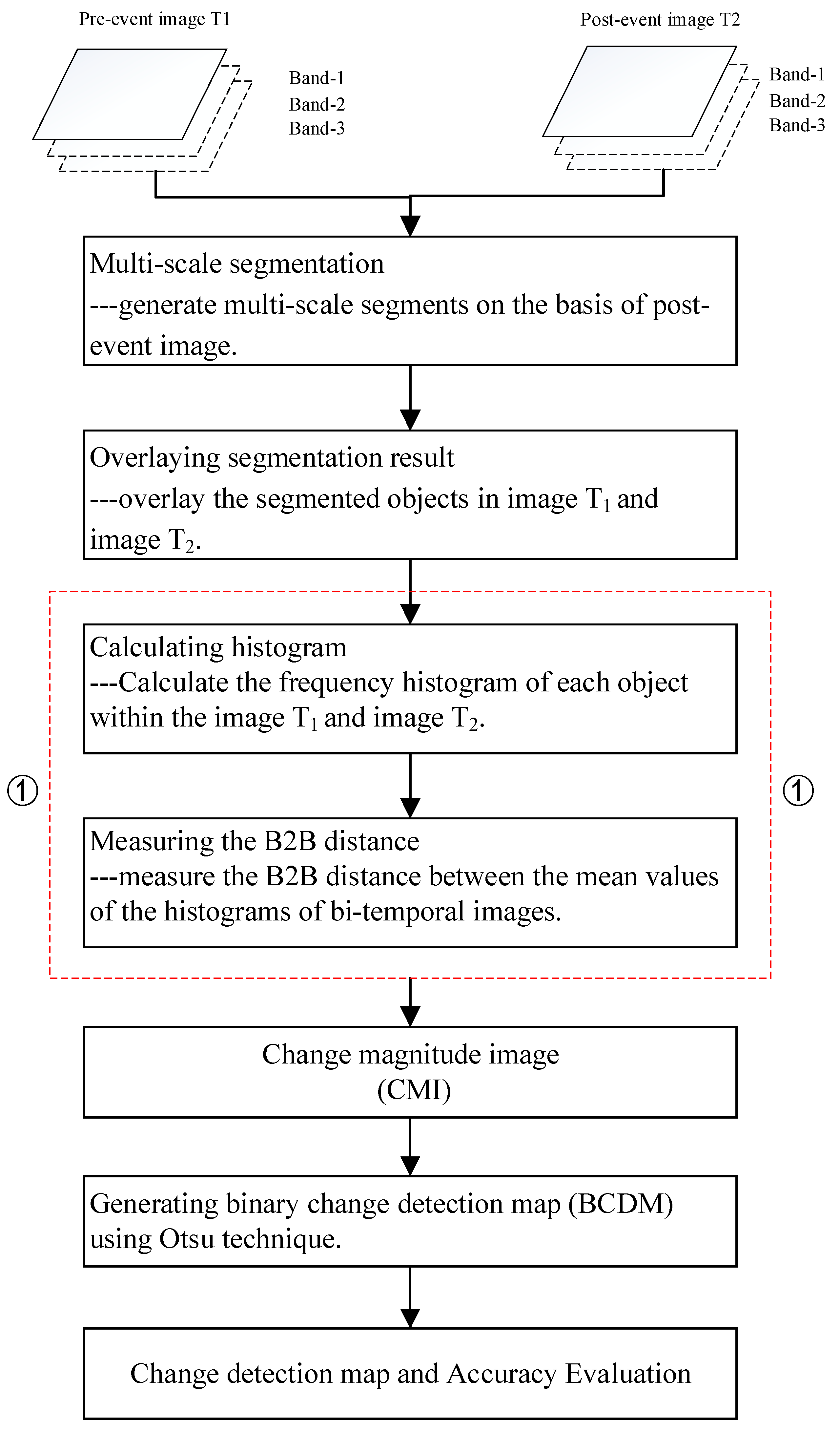
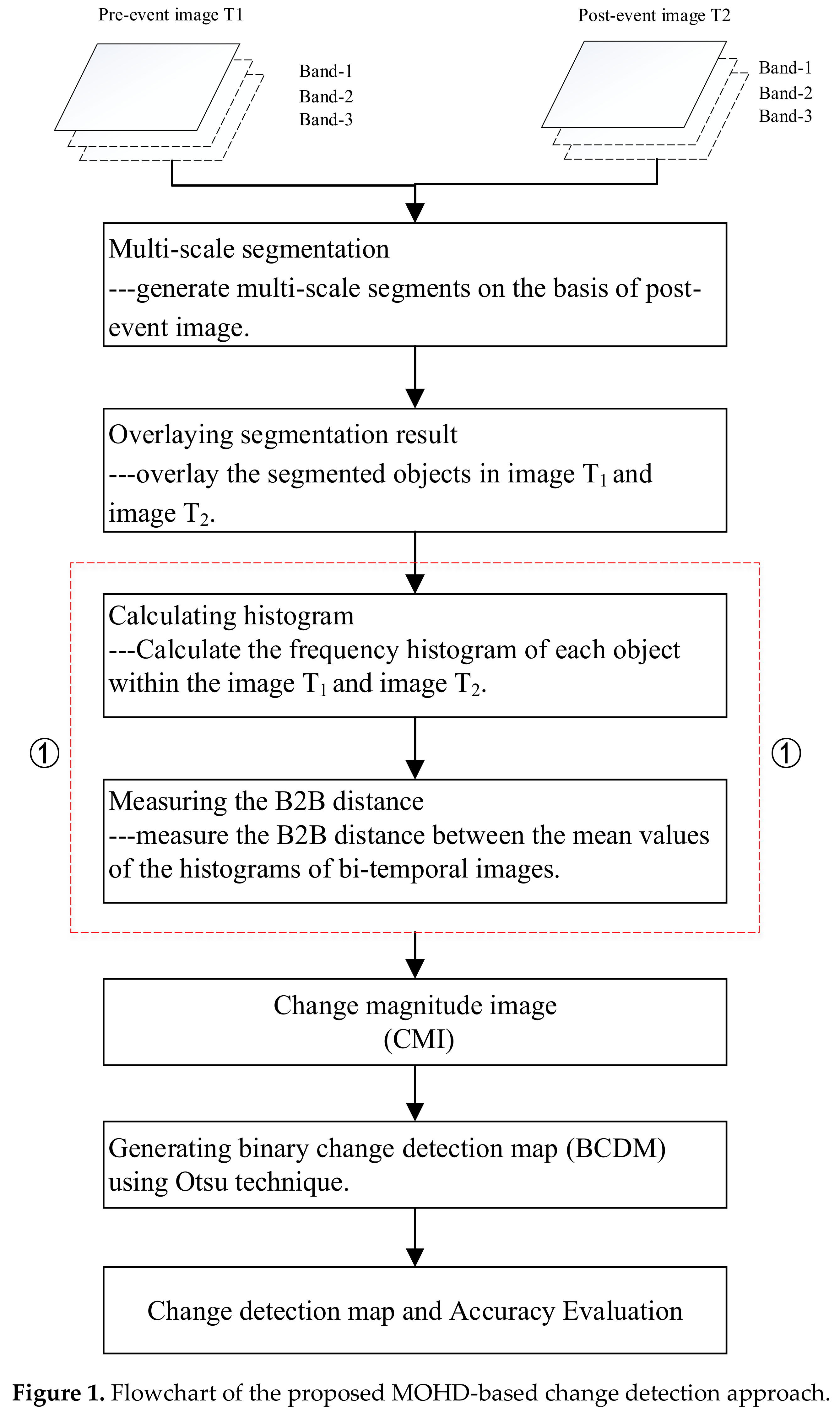
2. Proposed Multi-Scale Object Histogram Distance

The aim of the proposed MOHD lies in measuring the change magnitude through a spectral frequency distribution histogram of pairwise multi-scale objects. As shown in Figure 1, the proposed MOHD approach is composed of the following steps. (1) Multi-scale segmentation algorithm is applied to extract multi-scale objects based on the post-event image. Each object is then taken as a local region to extract histograms from the corresponding geographical area of bi-temporal images. (2) Histogram feature vector of the bi-temporal image is defined based on the frequency and spectral distribution. (3) B2B distance is promoted based on the definition of arithmetic frequency-mean feature (AFMF). In the following sections, details of the proposed MOHD are given when the change magnitude between bi-temporal images is calculated object-by-object and Otsu binary threshold is employed to divide the CMI into BCDM.

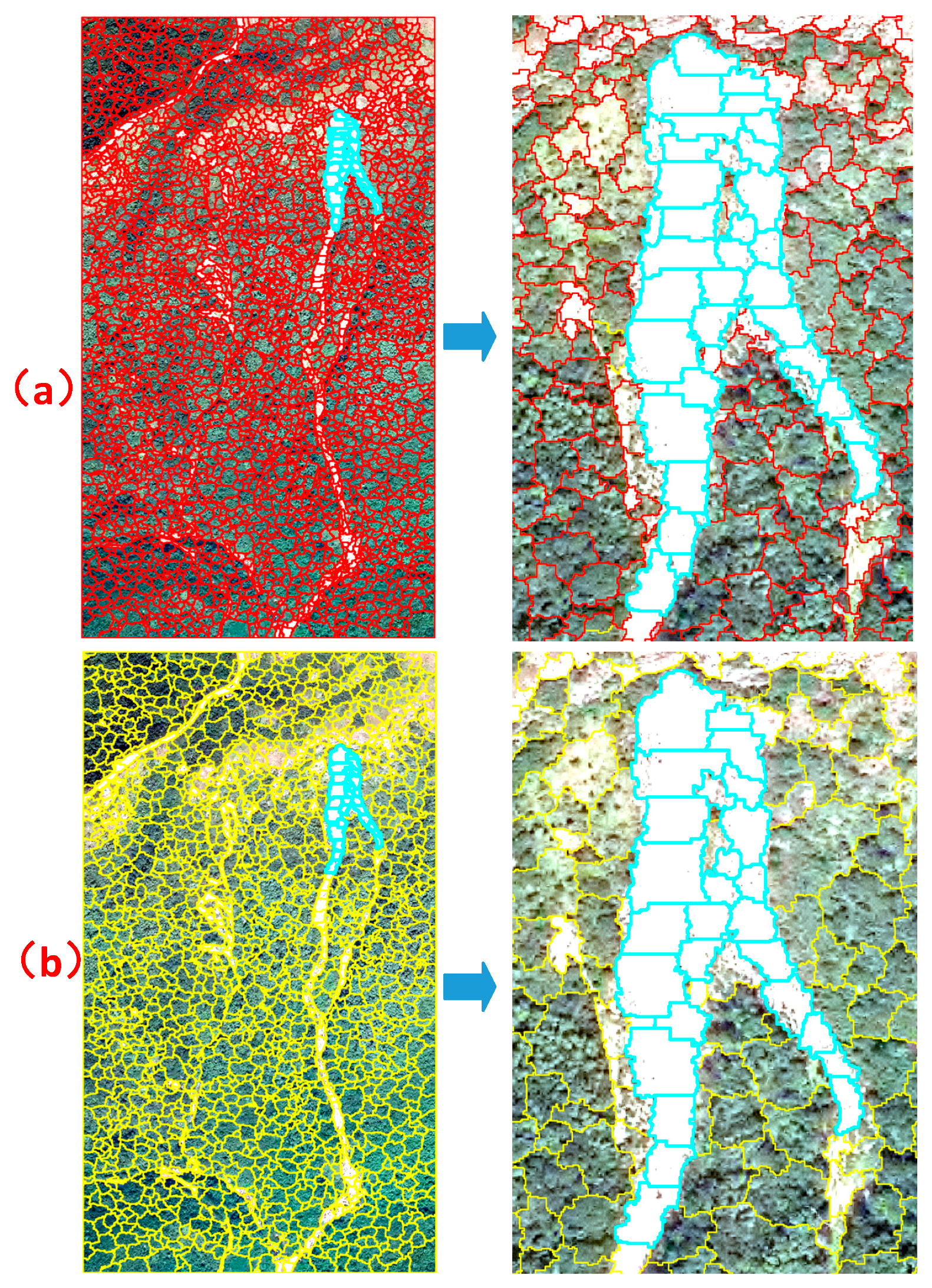
2.1. Brief Review of a Multi-Scale Segmentation Algorithm

In the proposed MOHD, multi-scale object extraction is a pre-condition for the continuous process. Herein, a widely used multi-scale algorithm called FNEA [35] is adopted in the proposed approach. FNEA generates the multi-scale object from a pixel, and the optimisation procedure attempts to minimise the average heterogeneity and maximise the respective homogeneity for the given number of image objects. The total count number of the objects for a given image is usually determined by the parameter of scale. In general, a multi-scale object for image analysis has three advantages [18,37,38]: (1) more image features can be utilised for land-cover classification or change detection compared with the pixel-based method; (2) object-based methods can reduce noise in the detection map; and (3) the segmental object has the ability to depict the shape, size and structure of a target. Given these advantages of object-based image analysis, in the proposed MOHD approach, multi-scale objects are extracted using the FNEA algorithm, which is embedded in the software eCognition 8.7. In addition, a tool called estimation of scale parameter (ESP) is suggested to estimate the multi-segmentation scale [39] for the adopted FNEA. Under this context, the object set $O_{T1}$ is first extracted from the pre-event image and defined as $O_{T1}=\left\{o_1^{t1},o_2^{t1},o_3^{t1}\dots o_n^{t1}\right\}$, and the object set $O_{T2}$ from the post-event image is defined as $O_{T2}=\left\{o_1^{t2},o_2^{t2},o_3^{t2}\dots o_n^{t2}\right\}$. Notably, $O_{T1}$ and $O_{T2}$ are equal in terms of total number and object shape in the spatial domain. However, the feature of each corresponding object is extracted from the corresponding temporal image. Generally, if a ground target in an area does not change, then histograms of the ground target in different images may have higher similarity in terms of shape, trend and statistical features. On the contrary, if the target changes from one to another, then histograms of the target area in different images will be different. For example, in the object-based histograms for the change and unchanged areas shown in Figure 2, the two left sub-figures are the histogram for an object in unchanged areas in the bi-temporal image, and the two right sub-figures are the changed areas. The histograms for the changed area are different, whereas the histograms for the unchanged area have high similarity.

To demonstrate the different performance of multi-scale segmentation with different scale-parameters, the segmental objects based on the dataset-A are shown in Figure 3. As the observation of the highlighted segments in Figure 3 shows, despite the fact that a different scale-parameter will generate different segments, the different segments depict the same shape and size of the landside area, preserving the same boundary of landslide area. Therefore, when the post-event segments are overlaid on the pre-event image, if a target is not changed, the shape and size can be depicted by the segments. Therefore, when we measure the change magnitude between the bitemporal images in the same segment, if there is no change, the change magnitude will be less. On the contrary, when the change occurs, the change magnitude will be larger.

2.2. Definition of Histogram Feature and OHD

Histogram feature and object histogram distance are defined in detail in this section. Firstly, pairwise objects $o_i^{t1}$ and ${\mathrm{o}}_i^{t2}$ are selected from the set. Then, the pixels within the pairwise objects are taken to construct the corresponding spectral frequency distribution histogram, and object $o_{\mathrm{i}}^{t1}$ is assigned $H_1^{t1}\left\{r\right\}$, $H_1^{t1}\left\{g\right\}$ and $H_1^{t1}\left\{b\right\}$ for the red, green and blue bands (R-G-B), respectively. Based on the assignments, an arithmetic frequency-mean feature (AFMF) for a histogram is quantitatively defined as follows:

$$m_r^{t1}=\frac{1}{S_n}{\displaystyle \sum }_{k=1}^{k=16}{f}_k\times p_k^m$$

(1)

where $m_r^{t1}$ is the AFMF spectral histogram feature of the histogram $H_1^{t1}\left\{r\right\}$. In the preceding definition, $f_k$ is the frequency of the k-th bin of the histogram $H_1^{t1}\left\{r\right\}$, and $p_k^m$ is the middle spectral value of the k-th bin. In addition, k is the count of bins for the histogram, with k ranging from 1 to 16. $S_n$ is the total number of pixels within the object $o_1^{t1}$. From the proposed defined equation of histogram feature, $m_r^{t1}$ indicates the mean expectation of the histogram, which is related to a group pixel within an object. In this manner, the mean spectral histogram feature for the R-G-B band can be obtained, and the feature vector can be given as $M_{o_i}^{t1}=\left\{m_r^{t1},m_g^{t1},m_b^{t1}\right\}$. Similarly, the feature vector for the other histogram is $M_{o_i}^{t2}=\left\{m_r^{t2},m_g^{t2},m_b^{t2}\right\}$.

On the basis of the feature definition of object-histogram for each band and inspired by the histogram distance promoted in the literature [22,40,41], B2B distance is promoted to measure the change magnitude between pairwise histograms through the aforementioned definition of AFMF. Therefore, B2B distance can be calculated as follows:

$$\Delta d_i=\frac{1}{2\times 3}{\displaystyle \sum }_{h=1}^{h=3}\Vert m_h^{t1}\left(i\right)-m_h^{t2}\left(i\right)\Vert$$

(2)

where $\Delta d_i$ is the B2B distance between the objects $o_i^{t1}$ and ${\mathrm{o}}_i^{t2}$. In addition, $m_h^{t1}$ and $m_h^{t2}$ represent the histogram mean of the h-band at pre- and post-event images, respectively. In general, the large $\Delta d_i$ demonstrates a large change between the area of the corresponding objects $o_i^{t1}$ and ${\mathrm{o}}_i^{t2}$.

Clearly, the CMI can be generated by mutually calculating the two multi-scale object sets, namely, $O_{T1}=\left\{o_1^{t1},o_2^{t1},o_3^{t1}\dots o_n^{t1}\right\}$ and $O_{T2}=\left\{o_1^{t2},o_2^{t2},o_3^{t2}\dots o_n^{t2}\right\}$, as discussed above. The proposed MOHD approach for measuring the change magnitude between bi-temporal VHR images is also promoted based on the following objective assumptions: (1) multi-scale segmentation based on the pre-event images is similar to that of the post-event images for the unchanged area; and (2) despite the pixels with high homogeneity within an object, these pixels are also very different in terms of their detailed spectral value, and the spectral mean frequency feature of an object’s histogram is regarded as the expected feature of the object.

2.3. Threshold for Obtaining Binary Change Detection Map

Apart from existing LCCD methods, a binary threshold is necessary to obtain the BCDM based on the CMI results. In the present study, a well-known automatic binary threshold named Otsu is preferred. Otsu is a widely used threshold approach in many existing LCCD methods [20,24]. Its main goal is to automatically compute a threshold via grey-level histograms to divide the CMI into the BCDM. In the proposed MOHD approach, a threshold is automatically determined by the Otsu approach to generate the BCDM and separate the CMI into a BCDM, which consists of two classes: Changed and unchanged.

3. Experiments and Analysis

Two VHR remote sensing images related to two land-cover change events were adopted in the experiments for comparison to test the performance of the proposed MOHD in LCCD. Additional details, including dataset description, experimental setting and comparison of results, are provided in the following sections.

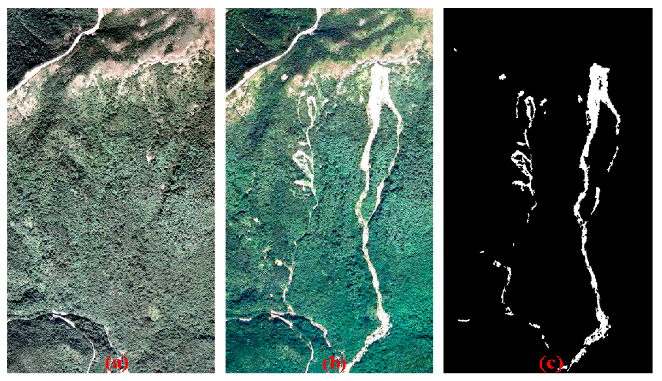
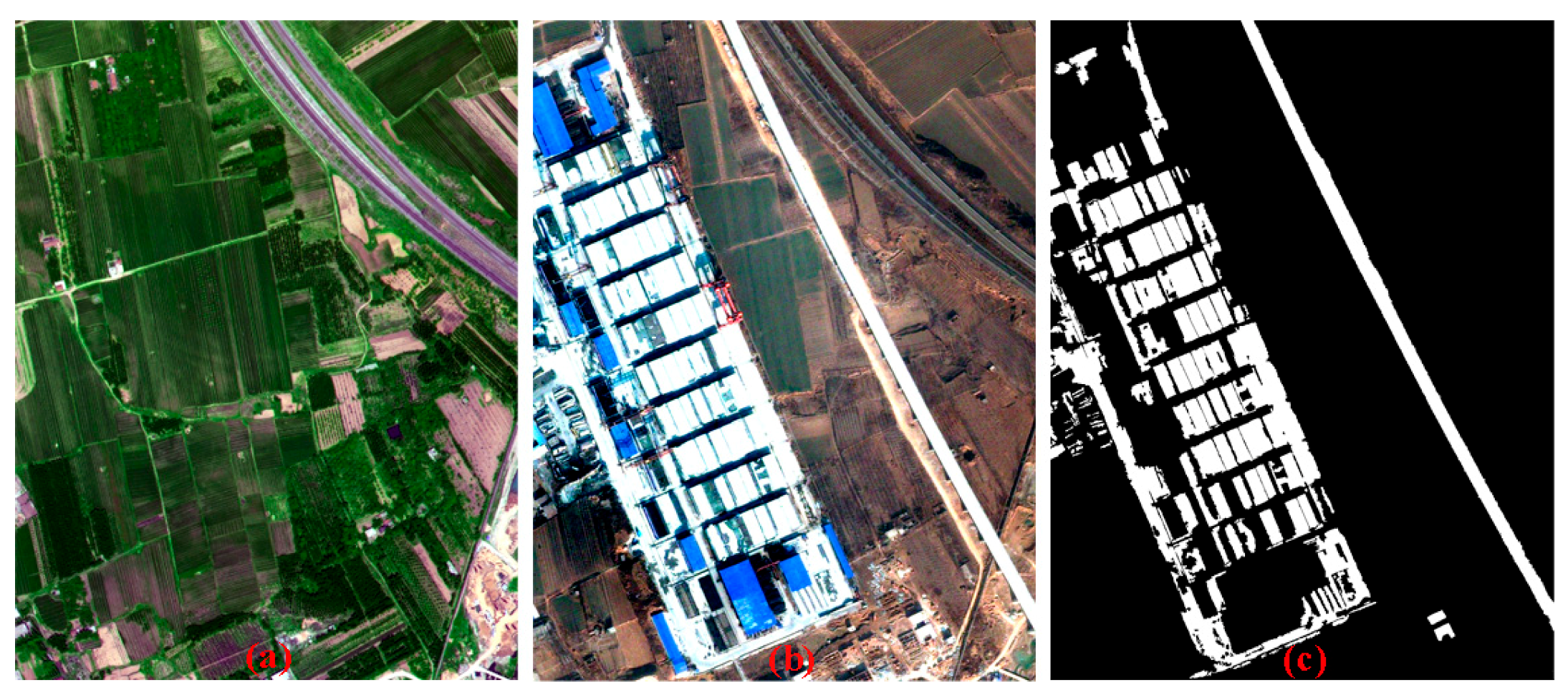
3.1. Dataset Description

The first dataset is a pair of aerial orthophoto images depicting a landslide change event in Lantau Island, Hong Kong, China. This dataset was acquired via a Zeiss RMK TOP-1 aerial camera in April 2007 and July 2014. The size of the dataset is 1252 × 2199 pixels with a spatial resolution of 0.5 m/pixel, as shown in Figure 4a,b. The ground truth image of the landslide area is shown in Figure 4c.

The second dataset depicts a land-use change event in Ji Nan City, Shan Dong Province, China. The pair images were acquired by the QuickBird satellite on April 2007 and February 2009. The size of the dataset is 950 × 1250 pixels with a spatial resolution of 0.6 m/pixel, as shown in Figure 5a,b. This change event is a typical scene in the countryside of developing China, with numerous plant-covered areas changed into buildings. The ground truth image of the dataset is generated by photo interpretation, as shown in Figure 5c.

3.2. Experimental Setting

Three LCCD methods, including two popular pixel-based methods and one relatively new object-based method, are compared with the proposed approach in this study to test the feasibility and effectiveness of the proposed MOHD approach for LCCD. The three methods are LSELUC [4], PCA-Kmeans [29] and MAC-OBCD [32], respectively. Furthermore, the parameters of each approach are optimised using the trial-and-error method to guarantee fairness of comparison. Details of the parameter setting and ground reference are provided in

Table 1. Parameter setting of each LCCD method for two datasets.

Method	Parameter Settings
	Dataset A	Dataset B
LSELUC [4]	S = 9	S = 3
PCA-Kmeans [29]	h = 9, s = 3	h = 3, s = 3
MAC-OBCD [32]	depth = 5, area = 3	depth = 5, area = 3
Proposed approach	Scale = 40, compactness = 0.8, shape = 0.9	Scale = 45, compactness = 0.8, shape = 0.9

and

Table 2. Details of ground reference pixels for each dataset.

Dataset No. of Unchanged Pixels		No. of Changed Pixels
dataset A	2,639,914	113,234
dataset B	987,017	200,483

, respectively.

3.3. Results and Analysis

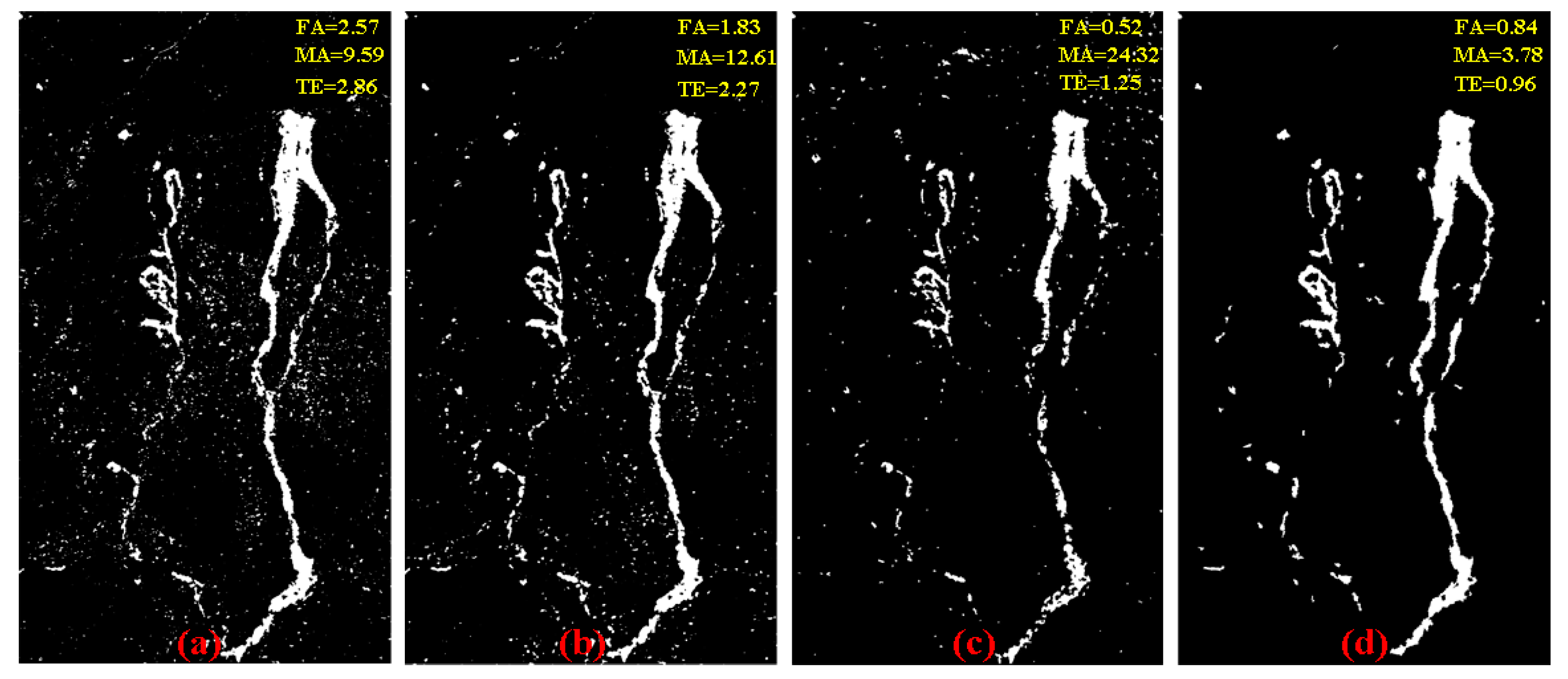
3.3.1. Evaluation Measurements

To quantitatively evaluate the accuracy and performance of each approach, the following three standard measures, which have been used in published literature [42], were employed: (1) false alarm rate (FA): $\mathrm{FA}=\frac{N_{uc}}{N_{TC}}\times 100\%;$ (2) missed alarm rate (MA): $\mathrm{MA}=\frac{N_{cu}}{N_{TU}}\times 100\%$; and (3) total error (TE):$\mathrm{TE}=\frac{N_{uc}+N_{cu}}{N_{TC}+N_{TU}}\times 100\%$, where $N_{uc}$ is the number of unchanged pixels detected as change pixels, $N_{TC}$ is the total number of changed pixels within THE ground reference map; $N_{cu}$ is the number of changed pixels detected as unchanged pixels; and $N_{TU}$ is the total number of unchanged pixels within the ground reference map.

3.3.2. Results Based on Dataset A

For dataset A, the BCDM is obtained by the proposed MOHD approach and three compared methods (Figure 6). From these figures of comparisons, the performance of the proposed MOHD approach demonstrated the least noise in the detection map compared with that of LSELUC [4], PCA-Kmeans [29] and MAC-OBCD [32]. When these approaches were compared in terms of quantitative accuracies, the proposed MOHD evidently achieved similar accuracies as well as MAC-OBCD [32] in terms of FA, accuracies which are better than those of LSELUC [4] and PCA-Kmeans [29]. However, the proposed MOHD clearly has superior outcomes to those of other approaches in terms of MA and TE. For example, the MA of the proposed MOHD decreased from 24.32% to 3.78% compared with that of MAC-OBCD [32].

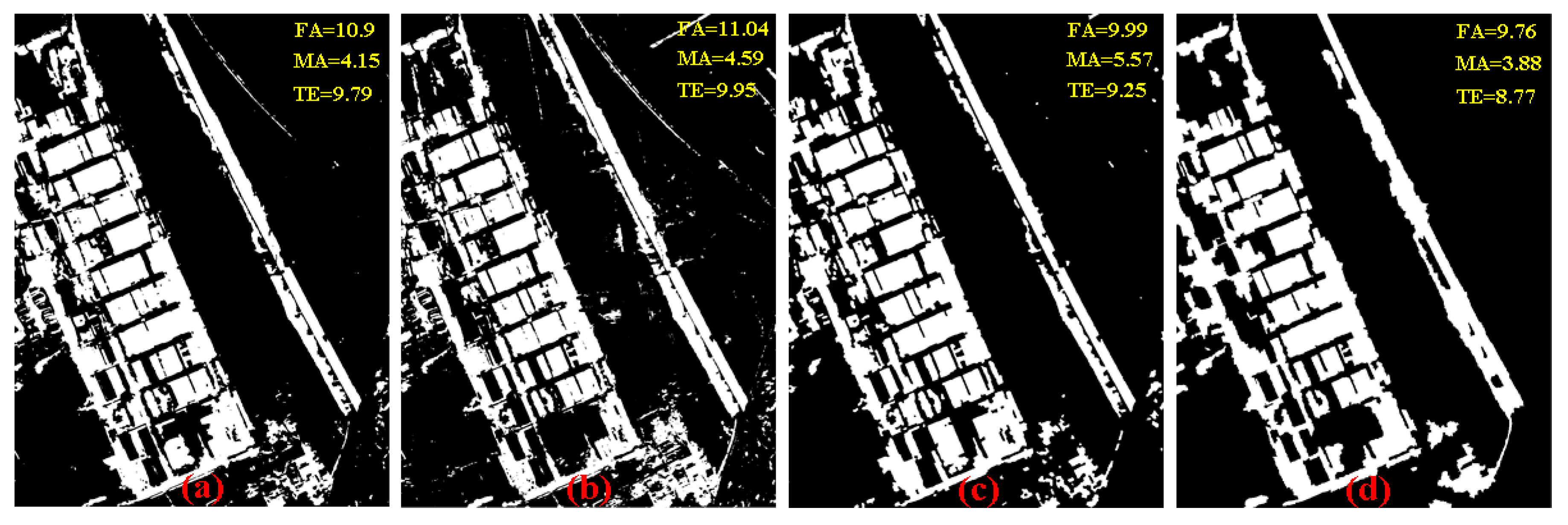
3.3.3. Results Based on Dataset B

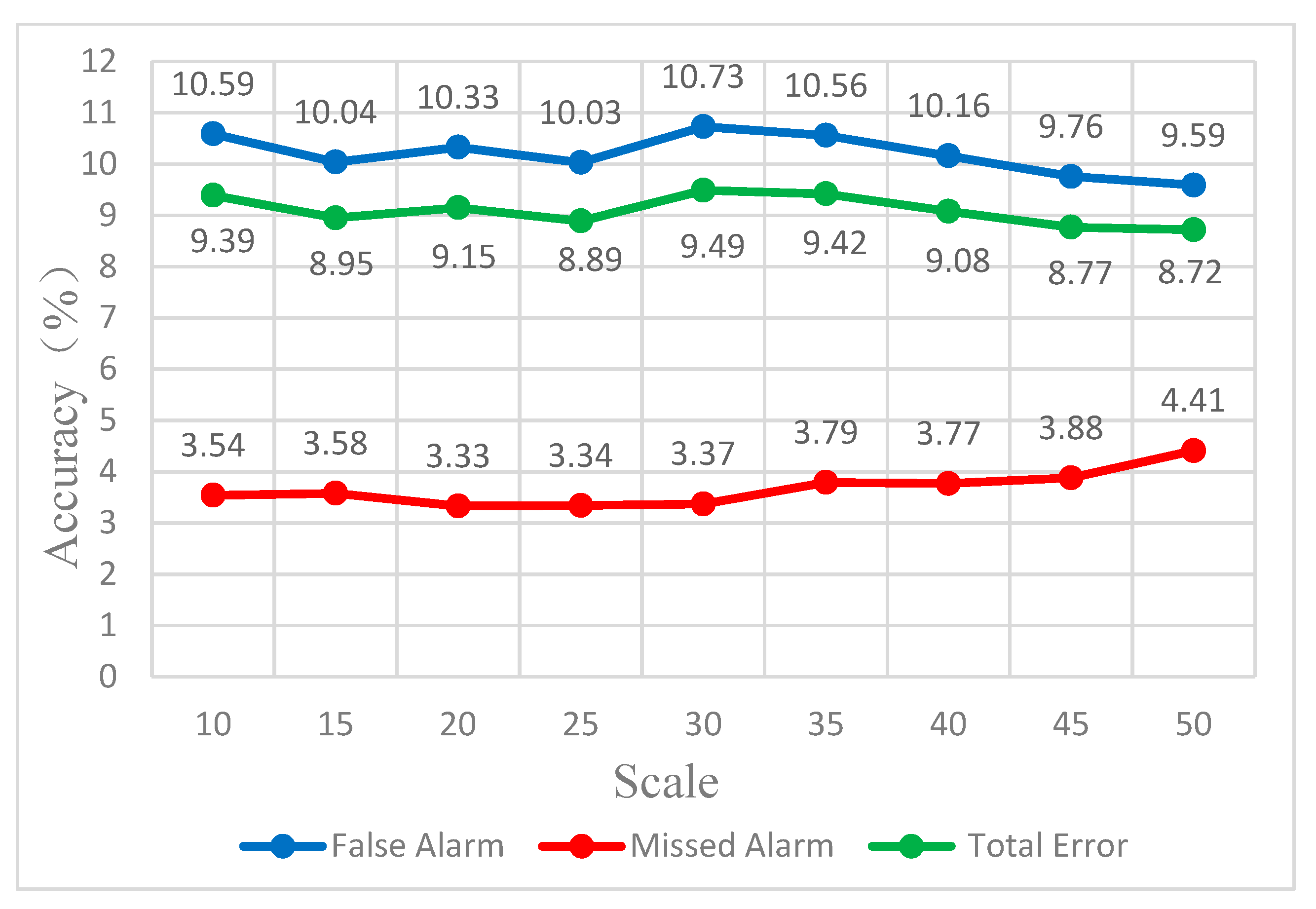
To further investigate the proposed MOHD approach, the comparisons based on dataset B with different LCCD methods are shown in Figure 6. These comparisons demonstrated that the proposed MOHD is superior to LSELUC [4], PCA-Kmeans [29] and MAC-OBCD [32]. For example, the FA of the proposed approach is 9.96%, which is the lowest false detection compared with that of other methods. This result means that the proposed approach can detect more changed pixels correctly. The detection results in Figure 7 indicate that the change detection map achieved by the proposed approach presents less noise.

To further investigate the relationship between segmentation scale and detection accuracy, we obtained a series of detection results using our proposed method with different scale parameters of multi-scale segmentation. Given that segmental objects with high homogeneity and regular shape are expected, the parameters of compactness and shape were fixed at 0.8 and 0.9, respectively. Under this context, Figure 8. shows the relationship between segmentation scale and detection accuracy for dataset B. The figure reveals that segmentation scale has a slight effect on the detection accuracy because it affects the number of segmental objects. Nevertheless, the inherent shape, structure and size of a given target will remain even when the number of segments for compositing vary. This is the fundamental characteristic of the multi-scale segmentation method [43]. For example, regardless of whether the area of a building in the image is depicted by different numbers of segmental objects, the shape, boundary and size will still be preserved and described by these different scale objects.

4. Discussion

From the preceding experiments, the proposed MOHD is found to be feasible and effective for detecting land-cover change using VHR remote sensing images. The performance of the proposed MOHD is competitive compared with the three existing and popular methods. Two aspects of the proposed approach are discussed below to promote its application in practice.

Firstly, the automatic degree of the different methods is discussed with the proposed MOHD. The preceding results show that LSELUC [4] has one necessary parameter(s), whereas PCA-Kmeans [29] and AMC-OBCD [32] have two parameters that must be determined. The optimisation parameters of an approach may vary with different LCCD datasets, and their determination is time consuming. Despite the relation of the proposed approach to three parameters in the pre-processing step of multi-scale segmentation, the determination of such parameters is convenient because the spectra and shape of multi-scale objects in the proposed MOHD approach are expected to be highly homogeneous and regular, respectively. Therefore, a relatively high shape and the compactness of FNEA in eCognition are provided to obtain the multi-scale object with high homogeneity and regular shape.

Secondly, the proposed MOHD has an expected balance in the three measurements of FA, MA and TE. Low values of the three measurements indicate satisfactory detection performance. However, in practical applications, the three measurements are usually in conflict with one another. For example, in the comparisons based on dataset A with different LCCD methods in Figure 4, although AMC-OBCD [32] achieved the best accuracies in terms of FA and TE compared with other approaches, the improvement of AMC-OBCD [32] in FA and TE was achieved at the expense of increasing MA. A similar conclusion can be obtained whilst analysing the quantitative results of LSELUC [4] and PCA-Kmeans [29] in Figure 4. When attention was focused on the values of MA, FA and TE in the proposed approach for the two datasets, the proposed MOHD demonstrated the best balance amongst the three measurements of detection accuracies in practical application. This balance is helpful for improving the usability of the proposed approach in LCCD using VHR remote sensing images.

On the basis of the preceding discussion, (1) the proposed MOHD is found to be feasible and effective for detecting land-cover change, and (2) the optimal parameter setting of the proposed approach is more easily determined than those of LSELUC [4], PCA-Kmeans [29] and AMC-OBCD [32]. Moreover, the proposed approach can balance the value of the three measurements of quantitative assessment. The aforementioned characteristics of the proposed MOHD approach are beneficial for practical application.

5. Conclusions

In this work, a novel method named MOHD which uses VHR remote sensing images is proposed for LCCD. Firstly, multi-scale objects based on pre- or post-event images are extracted through FNEA, and the histogram of each object is built according to the spectral distribution of pixels within the object. Secondly, an AFMF of the histogram is quantitatively defined for each histogram. Therefore, the CMI can be obtained by measuring the distance between a pairwise histogram in B2B distance. Finally, a classical binary threshold method named Otsu is employed to divide the CMI into BCDM. The contribution of the proposed MOHD can be summarised as follows.

(1)

The proposed MOHD approach can achieve competitive detection results. From the experimental results based on two real land-cover change events, the proposed MOHD approach evidently obtained better quantitative accuracies in terms of FA, MA and TE compared with those of LSELUC [4], PCA-Kmeans [29] and MAC-OBCD [32].

(2)

The proposed MOHD approach possesses an advantage in terms of usability. The preceding discussion clearly indicates that the parameter setting of the proposed MOHD is more convenient than that of existing methods, such as LSELUC [4], PCA-Kmeans [29] and MAC-OBCD [32]. The proposed MOHD can likewise achieve competitive results and simultaneously balance the contradiction amongst FA, MA and TE. The advantage of the proposed approach is beneficial for practical application, and the proposed MOHD approach has wide potential applications.

Despite the superiority presented by the proposed MOHD approach in certain aspects, it still has some limitations, such as the need to conduct multi-scale segmentation before it can be applied. However, determining the parameters for multi-scale segmentation depends on the experience of the practitioner. In future study, the focus will be on the automatic degree of determining the parameters for multi-scale segmentation. In addition, to test the generality of the proposed approach, it will be further investigated in another feature space. Furthermore, additional bi-temporal VHR image datasets must be collected, and the robustness of the proposed MOHD must be investigated through numerous remote sensing images referencing different land-cover change events.

References

1. Singh, A. Review article digital change detection techniques using remotely-sensed data. Int. J. Remote Sens. 1989, 10, 989–1003. [Google Scholar] [CrossRef]
2. Lu, D.; Mausel, P.; Brondizio, E.; Moran, E. Change detection techniques. Int. J. Remote Sens. 2004, 25, 2365–2401. [Google Scholar] [CrossRef]
3. Coppin, P.; Jonckheere, I.; Nackaerts, K.; Muys, B.; Lambin, E. Review articledigital change detection methods in ecosystem monitoring: A review. Int. J. Remote Sens. 2004, 25, 1565–1596. [Google Scholar] [CrossRef]
4. Zhang, X.; Shi, W.; Liang, P.; Hao, M. Level set evolution with local uncertainty constraints for unsupervised change detection. Remote Sens. Lett. 2017, 8, 811–820. [Google Scholar] [CrossRef]
5. Hansen, M.C.; Loveland, T.R. A review of large area monitoring of land cover change using landsat data. Remote Sens. Environ. 2012, 122, 66–74. [Google Scholar] [CrossRef]
6. Homer, C.; Dewitz, J.; Yang, L.; Jin, S.; Danielson, P.; Xian, G.; Coulston, J.; Herold, N.; Wickham, J.; Megown, K. Completion of the 2011 national land cover database for the conterminous united states–representing a decade of land cover change information. Photogramm. Eng. Remote Sens. 2015, 81, 345–354. [Google Scholar]
7. Wang, Q.; Yuan, Z.; Du, Q.; Li, X. Getnet: A general end-to-end 2-d cnn framework for hyperspectral image change detection. IEEE Trans. Geosci. Remote Sens. 2018, 24, 1–11. [Google Scholar] [CrossRef]
8. Zhu, Z.; Woodcock, C.E. Continuous change detection and classification of land cover using all available landsat data. Remote Sens. Environ. 2014, 144, 152–171. [Google Scholar] [CrossRef]
9. Anees, A.; Aryal, J. A statistical framework for near-real time detection of beetle infestation in pine forests using modis data. IEEE Geosci. Remote Sens. Lett. 2014, 11, 1717–1721. [Google Scholar] [CrossRef]
10. Macleod, R.D.; Congalton, R.G. A quantitative comparison of change-detection algorithms for monitoring eelgrass from remotely sensed data. Photogramm. Eng. Remote Sens. 1998, 64, 207–216. [Google Scholar]
11. Mas, J.-F. Monitoring land-cover changes: A comparison of change detection techniques. Int. J. Remote Sens. 1999, 20, 139–152. [Google Scholar] [CrossRef]
12. Xue, Z.; Du, P.; Feng, L. Phenology-driven land cover classification and trend analysis based on long-term remote sensing image series. IEEE J. Sel. Top. Appl. Earth Observ. Remote Sens. 2014, 7, 1142–1156. [Google Scholar] [CrossRef]
13. Yang, L.; Xian, G.; Klaver, J.M.; Deal, B. Urban land-cover change detection through sub-pixel imperviousness mapping using remotely sensed data. Photogramm. Eng. Remote Sens. 2003, 69, 1003–1010. [Google Scholar] [CrossRef]
14. Howarth, P.J.; Boasson, E. Landsat digital enhancements for change detection in urban environments. Remote Sens. Environ. 1983, 13, 149–160. [Google Scholar] [CrossRef]
15. Anees, A.; Aryal, J.; O’Reilly, M.M.; Gale, T.J. A relative density ratio-based framework for detection of land cover changes in modis ndvi time series. IEEE J. Sel. Top. Appl. Earth Observ. Remote Sens. 2016, 9, 3359–3371. [Google Scholar] [CrossRef]
16. Wang, L.; Sousa, W.; Gong, P. Integration of object-based and pixel-based classification for mapping mangroves with ikonos imagery. Int. J. Remote Sens. 2004, 25, 5655–5668. [Google Scholar] [CrossRef]
17. Myint, S.W.; Gober, P.; Brazel, A.; Grossman-Clarke, S.; Weng, Q. Per-pixel vs. Object-based classification of urban land cover extraction using high spatial resolution imagery. Remote Sens. Environ. 2011, 115, 1145–1161. [Google Scholar] [CrossRef]
18. Hussain, M.; Chen, D.; Cheng, A.; Wei, H.; Stanley, D. Change detection from remotely sensed images: From pixel-based to object-based approaches. ISPRS J. Photogramm. Remote Sens. 2013, 80, 91–106. [Google Scholar] [CrossRef]
19. Zhuang, H.; Deng, K.; Fan, H.; Yu, M. Strategies combining spectral angle mapper and change vector analysis to unsupervised change detection in multispectral images. IEEE Geosci. Remote Sens. Lett. 2016, 13, 681–685. [Google Scholar] [CrossRef]
20. Lv, Z.; Liu, T.; Zhang, P.; Benediktsson, J.A.; Chen, Y. Land cover change detection based on adaptive 2 contextual information using bi-temporal remote 3 sensing images 4. Remote Sens. 2018, 10, 901. [Google Scholar] [CrossRef]
21. Zhang, Y.; Peng, D.; Huang, X. Object-based change detection for vhr images based on multiscale uncertainty analysis. IEEE Geosci. Remote Sens. Lett. 2018, 15, 13–17. [Google Scholar] [CrossRef]
22. Bruzzone, L.; Prieto, D.F. Automatic analysis of the difference image for unsupervised change detection. IEEE Trans. Geosci. Remote Sens. 2000, 38, 1171–1182. [Google Scholar] [CrossRef]
23. Radke, R.J.; Andra, S.; Al-Kofahi, O.; Roysam, B. Image change detection algorithms: A systematic survey. IEEE Trans. Image Process. 2005, 14, 294–307. [Google Scholar] [CrossRef] [PubMed]
24. Otsu, N. A threshold selection method from gray-level histograms. IEEE Trans. Syst. Man Cybern. 1979, 9, 62–66. [Google Scholar] [CrossRef]
25. Hao, M.; Shi, W.; Zhang, H.; Li, C. Unsupervised change detection with expectation-maximization-based level set. IEEE Geosci. Remote Sens. Lett. 2014, 11, 210–214. [Google Scholar] [CrossRef]
26. Volpi, M.; Tuia, D.; Bovolo, F.; Kanevski, M.; Bruzzone, L. Supervised change detection in vhr images using contextual information and support vector machines. Int. J. Appl. Earth Observ. Geoinf. 2013, 20, 77–85. [Google Scholar] [CrossRef]
27. Ardila, J.P.; Tolpekin, V.A.; Bijker, W.; Stein, A. Markov-random-field-based super-resolution mapping for identification of urban trees in vhr images. ISPRS J. Photogramm. Remote Sens. 2011, 66, 762–775. [Google Scholar] [CrossRef]
28. Solano-Correa, Y.T.; Bovolo, F.; Bruzzone, L. An approach for unsupervised change detection in multitemporal vhr images acquired by different multispectral sensors. Remote Sens. 2018, 10, 533. [Google Scholar] [CrossRef]
29. Celik, T. Unsupervised change detection in satellite images using principal component analysis and k-means clustering. IEEE Geosci. Remote Sens. Lett. 2009, 6, 772–776. [Google Scholar] [CrossRef]
30. Silveira, E.M.; Mello, J.M.; Acerbi Júnior, F.W.; Carvalho, L.M. Object-based land-cover change detection applied to brazilian seasonal savannahs using geostatistical features. Int. J. Remote Sens. 2018, 39, 2597–2619. [Google Scholar] [CrossRef]
31. Dronova, I.; Gong, P.; Wang, L. Object-based analysis and change detection of major wetland cover types and their classification uncertainty during the low water period at Poyang lake, China. Remote Sens. Environ. 2011, 115, 3220–3236. [Google Scholar] [CrossRef]
32. Cai, L.; Shi, W.; Zhang, H.; Hao, M. Object-oriented change detection method based on adaptive multi-method combination for remote-sensing images. Int. J. Remote Sens. 2016, 37, 5457–5471. [Google Scholar] [CrossRef]
33. Dingle Robertson, L.; King, D.J. Comparison of pixel-and object-based classification in land cover change mapping. Int. J. Remote Sens. 2011, 32, 1505–1529. [Google Scholar] [CrossRef]
34. Blaschke, T.; Hay, G.J.; Kelly, M.; Lang, S.; Hofmann, P.; Addink, E.; Feitosa, R.Q.; Van der Meer, F.; Van der Werff, H.; Van Coillie, F. Geographic object-based image analysis–towards a new paradigm. ISPRS J. Photogramm. Remote Sens. 2014, 87, 180–191. [Google Scholar] [CrossRef] [PubMed]
35. Li, H.; Gu, H.; Han, Y.; Yang, J. An efficient multi-scale segmentation for high-resolution remote sensing imagery based on statistical region merging and minimum heterogeneity rule. In Proceedings of the International Workshop on Earth Observation and Remote Sensing Applications, EORSA 2008, Beijing, China, 30 June–2 July 2008; pp. 1–6. [Google Scholar]
36. Deng, F.; Yang, C.; Cao, C.; Fan, X. An improved method of fnea for high resolution remote sensing image segmentation. J. Geo-Inf. Sci. 2014, 16, 95–101. [Google Scholar]
37. Blaschke, T. Object based image analysis for remote sensing. ISPRS J. Photogramm. Remote Sens. 2010, 65, 2–16. [Google Scholar] [CrossRef]
38. Hay, G.J.; Castilla, G. Geographic object-based image analysis (geobia): A new name for a new discipline. In Object-Based Image Analysis; Springer: Berlin, Germany, 2008; pp. 75–89. [Google Scholar]
39. Drǎguţ, L.; Tiede, D.; Levick, S.R. Esp: A tool to estimate scale parameter for multiresolution image segmentation of remotely sensed data. Int. J. Geogr. Inf. Sci. 2010, 24, 859–871. [Google Scholar] [CrossRef]
40. Ratha, D.; De, S.; Celik, T.; Bhattacharya, A. Change detection in polarimetric sar images using a geodesic distance between scattering mechanisms. IEEE Geosci. Remote Sens. Lett. 2017, 14, 1066–1070. [Google Scholar] [CrossRef]
41. Zhuang, H.; Tan, Z.; Deng, K.; Yao, G. Change detection in multispectral images based on multiband structural information. Remote Sens. Lett. 2018, 9, 1167–1176. [Google Scholar] [CrossRef]
42. Lv, Z.; Liu, T.; Wan, Y.; Benediktsson, J.A.; Zhang, X. Post-processing approach for refining raw land cover change detection of very high-resolution remote sensing images. Remote Sens. 2018, 10, 472. [Google Scholar] [CrossRef]
43. Kim, M.; Warner, T.A.; Madden, M.; Atkinson, D.S. Multi-scale geobia with very high spatial resolution digital aerial imagery: Scale, texture and image objects. Int. J. Remote Sens. 2011, 32, 2825–2850. [Google Scholar] [CrossRef]
Figure 1. Flowchart of the proposed MOHD-based change detection approach.
Remotesensing 10 01809 g001
Figure 2. Object-based histogram demonstrations for change and unchanged areas, respectively.
Remotesensing 10 01809 g002
Figure 3. An example of multi-segmentation with different scale-parameter: (a) scale = 35, compactness = 0.8, and shape = 0.9; (b) scale = 45, compactness = 0.8, and shape = 0.9.
Remotesensing 10 01809 g003
Figure 4. First dataset A: (a) pre-event image obtained in April 2007; (b) post-event image in July 2014; (c) ground truth of the landslide area.
Remotesensing 10 01809 g004
Figure 5. Second dataset B: (a) pre-event image shot in April 2007; (b) post-event image shot in February 2009; (c) ground truth image of changed area.
Remotesensing 10 01809 g005
Figure 6. Binary change detection results with different LCCD methods for dataset A: (a) LSELUC [4]; (b) PCA-Kmeans [29]; (c) MAC-OBCD [32]; (d) the proposed MOHD approach; the accuracies of FA, MA and TE are presented in percentage (%).
Remotesensing 10 01809 g006
Figure 7. Binary change detection results with different LCCD methods for dataset B: (a) LSELUC [4]; (b) PCA-Kmeans [29]; (c) MAC-OBCD [32]; (d) the proposed MOHD approach; the accuracies of FA, MA and TE are presented in percentage (%).
Remotesensing 10 01809 g007
Figure 8. Relationship between segmentation scale and detection accuracy for dataset B.
Remotesensing 10 01809 g008