Abstract
Pencil-beam Doppler scatterometers are a promising remote sensing tool for measuring ocean vector winds and currents from space. While several point designs exist in the literature, these designs have been constrained by the hardware they inherited, and the design is sub-optimal. Here, guidelines to optimize the design of these instruments starting from the basic sensitivity equations are presented. Unlike conventional scatterometers or pencil-beam imagers, appropriate sampling of the Doppler spectrum and optimizing the radial velocity error lead naturally to a design that incorporates a pulse-to-pulse separation and pulse length that vary with scan angle. Including this variation can improve radial velocity performance significantly and the optimal selection of system timing and bandwidth is derived. Following this, optimization of the performance based on frequency, incidence angle, antenna length, and spatial sampling strategy are considered. It is shown that antenna length influences the performance most strongly, while the errors depend only on the square root of the transmit power. Finally, a set of example designs and associated performance are presented.
1. Introduction
Ocean surface currents and winds are essential climate variables that play a key role in air-sea interactions. They are tightly coupled since the winds drive the currents, while the currents provide a moving reference frame for momentum transfer from the atmosphere into the ocean, as well as transporting heat that modifies the air-sea boundary layer. The importance of measuring both parameters simultaneously has been recognized in the latest report from the National Academy of the United States [1] for NASA’s Earth Science activities in the 2020’s. This report also recommends the use of Doppler scatterometers as an instrument that would meet the science community observation needs in a potential moderate-cost Earth Explorer mission.
Chelton et al. [2] have examined the sampling and accuracy requirements needed for a satisfactory estimates of surface currents and their derivatives from a global ocean surface currents mission. They conclude that frequent temporal sampling (i.e., once a day or more frequently) is required to minimize the aliasing of rapid changes in the atmosphere and the ocean’s surface. They also conclude that high-resolution (5 km or better) spatial sampling is required for the estimation of surface derivatives, even if the final results are averaged to a lower resolution. Finally, they show that there would be substantial benefits to our present knowledge if the surface components were measured with a precision of 0.5 m/s or better at 5 km posting. Further reducing the noise to ∼0.2 m/s would have significant benefits in achieving proper space-time sampling of the ocean short mesoscale regime (30 km and smaller).
The design criteria for imaging pencil-beam Doppler scatterometers has been considered by Spencer et al. [3], and implemented as part of NASA’s SMAP mission. For imaging, a fixed Pulse Repetition Frequency (PRF) was selected to sample the Doppler bandwidth at broadside. Subsequently, Bao et al. [4] examined a point design for a Ku-band surface winds and currents that used a two-frequency approach to mitigate range ambiguities (although they did not examine in detail the impact of correlation on forming pulse-pairs using non-overlapping bandwidths). The design was updated to a dual-frequency Ku/Ka-band instrument in [5]. Bourassa et al. presented a Ka-band design for a potential Winds and Currents (WaCM) mission [6], but this design was constrained to use a single PRF because of EM compatibility with another instrument. Finally, Ardhuin et al. [7] have proposed the Sea Surface KInematics Multiscale (SKIM) monitoring concept, a modification of the near-nadir () wave spectrometer concept initially proposed by Jackson [8] to include Doppler information using a Ka-band multi-beam system. This concept is currently under evaluation by ESA as a potential mission to be selected in 2019 for flight in the mid-2020’s. While all of these systems measure surface currents, SKIM measures surface wave spectra, while the other two systems are designed to measure surface winds. Notice that we do not address here the optimization of SAR systems, such as SEASTAR [9], or multiple antenna fan-beam systems [10,11,12], since these systems have significantly different architectures and fixed Doppler bandwidths, unlike the variable bandwidth that results from a spinning antenna.
While all of these designs optimized system parameters within the capabilities of their hardware, they selected the system timing and bandwidth based on optimizing the signal-to-noise ratio (SNR) and satisfying the requirement of sampling the broadside Doppler spectrum. In [13], we examined the error budget for DopplerScatt, an airborne Doppler scatterometer, and derived a full system error budget. In this paper, I show that analysis of the error budget suggests that it is possible to optimize two key system variables, the system bandwidth and the inter-pulse period, independently of other system parameters. This is important because, while basic parameters, such as system power, are usually set by hardware constraints, system bandwidth and timing are often flexible in a design. In Section 2 and Section 3, I derive optimal analytic and numerical values for these two parameters. In Doppler scatterometry there is a natural competition between pulse-to-pulse correlation, which is maximized for short pulses with small separation, and minimizing the white noise amplification that occurs when the pulse separation goes to zero. Small pulse separations also have the disadvantage that the energy in each pulse is small due to the small pulse duration. These competing tendencies can be optimized and have a well-defined optimal solution for both the bandwidth and the pulse separation. The optimal solution leads inexorably to the need to vary the pulse length and pulse separation as a function of the pencil-beam scan angle.
After bandwidth and pulse separation are set optimally, we proceed to examine in Section 4 the selection of other system parameters: the radar frequency, incidence angle, and space-time mapping constraints. These results point to the importance of antenna length as the single most sensitive parameter in optimizing the performance after selecting the system timing and bandwidth.
Finally, in Section 5, all of these strands are brought together in a set of design examples that are examined to exhibit their sensitivity to antenna length and transmit power. The resulting performance is compared against the sampling goals in Chelton et al. [2].
2. Optimizing Doppler Scatterometer Parameters Given SNR
Burst-mode operations is the most flexible way to transmit many closely separated pulses, as required for Doppler estimation, and henceforth burst-mode operations will be assumed. Figure 1 illustrates burst-mode timing and defines some key variables used below. This assumption is consistent with various designs that have been presented in the literature [4,6,7]. However, especially for small range footprints, interleaved mode operations can present advantages [3], although the design of system timing can be more onerous and orbit dependent. The results presented below are easily generalized to interleaved pulsing, and lead to similar conclusions, but the variable inter-pulse-period (IPP) advocated here may be harder to optimize for interleaved systems.
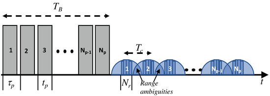
Figure 1.
Burst-mode timing diagram conventions. chirped pulses with inter-pulse duration separation (gray) are transmitted during a transmit cycle of duration , and the return pulses (blue) are range compressed so that the duration of the return pulses is dominated by the illuminated swath. It is assumed that the interval between transmit pulses is minimized, and the pulse duration, , obeys . (To get the exact results below, multiply the SNR by .) To form the measurement of interest, range samples are averaged for each received pulse (blue). Additional looks are obtained by averaging over the return pulses, but, since pulses are correlated for times smaller than , only independent samples are obtained. In general, for fast pulsing, there will be overlaps (range ambiguities) for parts of the received pulse, limiting the useful swath.
2.1. Error Models
2.1.1. Measurement Noise and Wind Speed Error
The intrinsic multiplicative measurement noise of scatterometer systems is characterized by parameter [3,14,15], defined by
where is the standard deviation of the radar cross section relative to the mean.
Given that we know the variability of the measured , what can be said about the errors in the retrieved speed, v, and direction, ? The detailed answer depends on the specific algorithms used in the retrieval, and can only be fully characterized using simulated data. However, it is possible to obtain simple bounds on the error that help to optimize the system design. The most sophisticated bound is obtained using the Cramér-Rao bound [16]. To optimize the scatterometer design, we notice that the wind speed estimation performance depends on the system parameters, while the wind direction accuracy is mainly determined by the azimuth viewing geometry. Thus we look for radar designs that will optimize the wind speed estimate, and assume that the wind direction is known.
Assuming that one has a geophysical model function (GMF) relationship, , where v is the wind speed, and is the direction, and assuming that the error in is small enough that one can expand around a the true speed and direction, one has
If one assumes that the direction is known (), the speed error is given by
so that the speed standard deviation is linearly dependent on . For Ku and Ka-bands, it is well known [13,17,18,19] that, for a given direction, the geophysical model function has a power-law dependence on wind speed
where A and have a weak dependence on wind speed. Taking the derivative with speed, one has
Replacing this into Equation (3), one finds the simple relationship
i.e., the fractional speed error is (up to a multiplicative constant) directly proportional to . As an example, Figure 2 shows that the incidence angle V-pol wind speed dependence reported in [13] is well matched by a quadratic function for winds below ∼20 m/s, although for Ku-band a decrease of for higher winds speeds is well documented. For near-nadir instruments with incidence angles ∼, such as SKIM [7], , and there is insufficient wind sensitivity to make a good wind speed estimates.
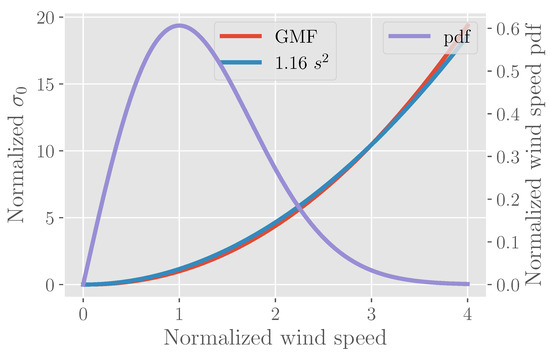
Figure 2.
Ka-band (not in dB) averaged over all azimuth angles divided by ∼ 7.8 × 10 (∼−22 dB), the cross section of the most likely wind speed value, m/s, as a function of the wind speed divided by . (Red line) Data from [13]; (Blue line) Quadratic fit. (Purple line) Rayleigh distribution of normalized wind speed.
2.1.2. Radial Velocity Errors
Doppler scatterometers measure the radial velocity along the line of sight by forming pulse-pair interferograms and, after subtracting the platform motion contribution, relating the measured phase difference, , to the radial velocity from the moving ocean, , by
where is the electromagnetic wavenumber, and is the pulse pair time separation [13]. In [13] we derive, and validate experimentally, the radial velocity random error variance,
where is the number of range looks, as above; is the number of independent pulse pair samples in occurring when averaging over a time , which corresponds to the burst time for a space borne burst mode system. In [13], we showed that , where is the pulse pair correlation time, which does not depend on and is only very weakly dependent on , for moderate or high SNR. Henceforth, we will assume that can be ignored in the optimization of the bandwidth and inter-pulse period. Finally, is the pulse-pair correlation which is the product of a thermal noise contribution, ; an ocean correlation time contribution, ; and a contribution from the azimuth variation of the Doppler over the footprint,
where ; is the correlation time for the ocean, which for Ka-band is greater than 2 ms; is the azimuth angle relative to the platform velocity vector; and is the broadside Doppler correlation time, which, for a Gaussian two-way antenna pattern of azimuth standard deviation and a platform velocity , is given by . This can be approximated by
where L is the antenna length, and the one-way half-power beamwidth is given by (for reflectors 1.1–1.2)). The and product can be combined as
where is the pulse-to-pulse signal correlation time. To achieve good pulse-to-pulse correlation, one chooses , so, except for angles close to the velocity vector, where , one has , which implies that the correlation time (or inverse Doppler bandwidth) increases significantly away from the broadside direction, achieving a maximum value of , the water correlation time.
2.2. Optimizing
In the previous section, we saw that, for each wind speed, one can optimize the radar performance by minimizing . For situations where the error introduced by the noise calibration is much smaller than that given by the measurement noise (the usual situation), one can approximate [3,14,15,20]
where and are the number of range and burst looks discussed above, and is the system signal-to-noise ratio. Given X, the desired resolution after range look averaging, the number of range looks as a function of the system bandwidth, B, and the incidence angle, , is given by
where is the minimum bandwidth, the bandwidth required to resolve a range slice of size X with a single look. To first order, the number of azimuth looks, , is independent of the system bandwidth, and depends mainly on the cross-track distance, the antenna rotation speed, etc. Finally, the SNR depends on the bandwidth through three factors: (1) the thermal noise is linearly dependent on the bandwidth; (2) the range compression gain is linearly dependent on the bandwidth and cancels the thermal noise contribution; (3) finally, the scattering area is inversely proportional to the bandwidth, leading to the conclusion that the SNR is inversely proportional to the bandwidth, which is simply a statement of energy conservation. This behavior is summarized by writing the SNR as
where is the signal-to-noise ratio achieved when the bandwidth is set to , i.e., when there is only a single range look per slice. Replacing this dependence into Equation (15) results in an equation giving the explicit dependence of on the number of range looks (or, equivalently, the bandwidth)
where is the noise-to-signal ratio (NSR). This equation can be used to obtain the optimal value for taking the derivative of with respect to and setting the results to zero. The result is , where is the optimal value for . Using Equation (18), the optimal number of range looks, , is given by the simple relation
Notice that when the optimum number of looks is taken, one has that , and the lowest achievable value of is given by
The behavior of is shown in Figure 3. The normalized reaches a minimum of 1 when , increases rapidly (as ) for , and increases more slowly (as ) for . The implications of this figure for the choice of bandwidth is that the fractional speed error performance degrades quickly when the number of range looks is smaller (smaller bandwidth) than the optimal, but degrades more slowly when a larger number of looks (larger bandwidth) are selected. This implies that when considering system design, it is better to sin in the direction of too large a bandwidth rather than too low a bandwidth.
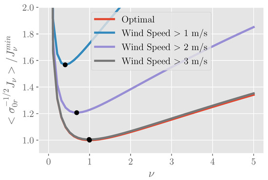
Figure 3.
Ratio of to the minimum achievable value of as a function of and for lower wind speed thresholds of 1 m/s (aqua), 2 m/s (magenta), and 3 m/s (gray). In red is the optimal curve given in Equation (20). The location of the optimal is indicated by a circle. For Equation (20), the optimum , but the optimum value becomes smaller when the wind speed distribution is accounted for, as in Section 3.
2.3. Optimizing Radial Velocity Variance
To optimize the radial velocity, we must optimize simultaneously and given , the noise-to-signal ratio (NSR). For a given burst time, , one can make the good approximation that the burst has approximately pulses, and that the SNR for a given pulse will be proportional to . Separating the dependence on range looks and inter-pulse period, the NSR, , can be written as
where is the NSR for one range look and one pulse transmitted per burst. The radial velocity standard deviation equation can then be written as
The radial velocity standard deviation depends on the system parameters we are trying to optimize through the function , which is shown in the upper left corner of Figure 4. Unlike the results of the previous section, this cannot be solved completely analytically since it involves transcendental functions. However, as shown in Appendix A, one can solve for in terms of , and solve for numerically using an efficient iteration scheme or simple 1-dimensional Newton root finder. The final result is
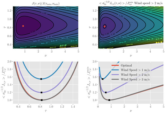
Figure 4.
(Upper row) Two dimensional of the optimal function as a function of and for Equation (25) (left) and for the wind averaged case (right), Equation (34), choosing a threshold wind speed of 2 m/s (c.f., Section 3). (lower row) Cross sections at optimal (left) and optimal (right) for the optimal case (red), and for various lower wind-speed thresholds: of 1 m/s (aqua), 2 m/s (magenta), and 3 m/s (gray).
Thus, the recipe for optimizing the parameters consists in first choosing , which will result in a single look NSR of . The next step consists in taking a number of range looks , which almost the same number of looks as prescribed by Equation (21), considering that is the one-look SNR for a pulse train of pulses.
The results obtained by minimizing the radial velocity error differ significantly from those obtained if one only requires that the pulse-to-pulse phase error be minimized. Following a process similar to the one outlined above, the optimal parameters for minimizing the phase error are found to be , , corresponding to , , , and , so there is a 50% degradation in the expected performance. On the other hand, for the “optimal” parameters, one has , , . These parameters are optimal assuming that Equation (8) is accurate for all values of . In fact, this equation breaks down for small values of the correlation. Examining the error surfaces shown in Figure 4, one sees that the dependence away from is not very strong up to ; similarly, is not very sensitive up to ; in fact, making this choice results in , , , and , so that only a 5% performance degradation occurs, while is sufficiently high so that Equation (8) applies reliably. These values may not be optimal, and are only provided for illustrative purposes. While they make the estimate more robust, they also increase the range ambiguities, as will be examined in greater detail below.
The fact that has a single optimal value has important implications for the optimal inter-pulse period, , which will now depend on the azimuth angle relative to the platform motion:
To date, the designs proposed ([4,6,7]) have assumed a fixed value fixed, , with a corresponding non-dimensional . In Figure 5, I plot , which represents the fractional increase in relative to the optimum, assuming that the optimal number of range samples is taken and is set to , the optimal value at broadside.
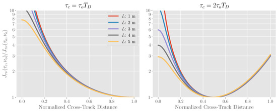
Figure 5.
Degradation in performance in for fixed PRF relative to the value where the PRF is allowed to vary as a function of scan angle for varying antenna length L. On the left panel, the PRF is optimized for broadside viewing (e.g., as in SKIM), while, on the right, it is optimized to have lowest error in the mid-swath. As can be seem, performance can degrade by close to an order of magnitude for the worst scan angles if the PRF is not varied over the scan. A temporal correlation time of 1 ms was used for these calculations.
3. Optimizing Doppler Scatterometer Parameters over Winds
Optimizing Wind Estimates
To optimize the performance across the entire wind speed spectrum, it is necessary to use, , the probability distribution function (pdf) for wind speeds. Freilich and Challenor [21] indicate that a distribution fitting the observed data is the Rayleigh distribution, given by
where is the normalized speed, m/s is the most likely wind speed (mode of ), the mean wind speed is given by m/s and the median speed is m/s. The pdf for s is plotted in Figure 2.
It should be noted that the most likely value of does not correspond to the value of : rather, the most likely value is . This can be seen very clearly when : a simple change of variables shows that is exponentially distributed:
where , is the backscatter cross section relative to . While the most likely value of , the mean will be , or , and the median will be a factor of greater than . Since the errors are singular for vanishing SNR, it is not be meaningful to speak of the performance for all winds, including very small values. In any case, the coupling between winds and backscatter breaks down at about 2 m/s wind speeds, when small capillary waves are no longer generated by local winds [22]. The analysis below will therefore be limited to winds above a certain threshold, and we will examine the dependence of the performance on this minimum speed threshold value.
To derive the optimal system parameters when the wind distribution is taken into account, we note that the NSR is inversely proportional to the relative cross section, , and the performance bounds can be written as
where is the NSR for the maximum likelihood winds, and the commonly used scene independent “noise-equivalent ” for the one-look system, , has been introduced to decouple system parameters from ocean surface brightness.
To derive the optimal parameters, we require that the average over all winds greater than be minimized for or . These averages will only depend on the wind through integrals of the form
where J is either (independent of ), or . Unfortunately, there does not appear to be a nice analytic approach for minimizing these functions, but they are smooth, with a single minimum (see, for example Figure 3, upper left) and easily minimized using standard packages. For illustration, we present below results for V-pol Ka-band at incidence angle using the wind GMF in [13].
The results for and various wind speed minima are shown in the lower panels of Figure 3, while those for are shown in Figure 4. For , when m/s, , , and for m/s, , . These results show that the optimal value of is the same for all cases, which makes sense since the signal correlation is independent of scene brightness, and depends only on the ratio of the pulse repetition sampling to the Doppler bandwidth. The number of range looks that can be taken is highly dependent on SNR, and therefore shows wind threshold dependence for both figures of merit, and leads to a worsening of the expected performance when averaging over wind relative to the case where the bandwidth was optimized for a single value of SNR. However, even when all winds down to 2 m/s are allowed, the performance degradation for the best parameters is only of 20% relative to the performance at the mode wind speed. In general, it seems preferable not to take as many range looks as the SNR at , would indicate that a number between 0.6 and 0.7 times the SNR would be more robust.
The impact on the and performance as a function of wind speed is shown in Figure 6, for both the optimal parameters at various wind speed thresholds and for and parameters selected to increase the expected correlation above a certain level, as discussed in the previous section. The results for both error sources is very similar: the performance improves slowly for speeds greater than , while it degrades quickly for values below. This is due to the proportionality of both to , which, using Equation (4), implies that the errors are multiplied by a factor of , which becomes singular as , while decreasing slowly for . The figure also shows that the performance is not terribly sensitive to the exact choice of and , as long as these parameters are not varied too far from their optimal values. This allows the selection of values for in the regime of applicability of Equation (8), and also allows some flexibility to accommodate for engineering design constraints.
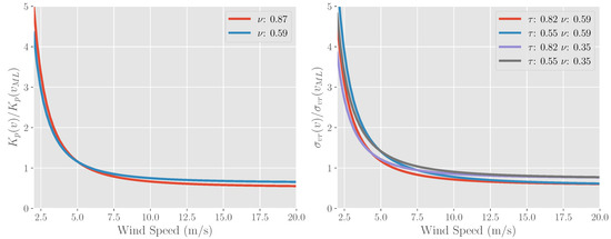
Figure 6.
(left) Ratio of as a function of wind speed to for the maximum-likelihood wind velocity for the optimal value of and a lower value representing lower bandwidth: the performance is robust to picking the bandwidth; (right) ratio of the radial velocity as a function of wind speed to the radial velocity at the maximum-likelihood wind for various values of .
4. Other Design Considerations
Since the wind and current sampling requirements have similar behavior for the number of looks, we concentrate here on the current requirement that poses additional constraints. Using Equations (14), (33), and (34), one can write the equation for the expected surface-projected radial velocity (i.e., ) standard deviations as
where is the 3-dB antenna azimuth beamwidth. The term , where is the antenna azimuth resolution and is the final azimuth resolution to which the data are averaged, accounts for the change of number of independent samples when averaging the footprint data to a lower resolution, and is introduced so that systems with different azimuth footprints can be compared consistently.
4.1. Frequency and Polarization
For a given antenna length, the surface-projected radial velocity in Equation (35) depends linearly on the wavelength through the antenna azimuth beamwidth. This is a strong constraint and implies that, given an antenna size and other terms being equal, the radial velocity error will be 2.7/6.4/28.6 times smaller at Ka-band than at Ku/C/L-bands. Higher transmit powers are more easily achieved at lower frequencies with current technology, reducing , but, for a given incidence angle, the backscatter cross section decreases with decreasing wavelength, so from power considerations it is also generally beneficial to choose smaller wavelengths in the design. The only term in Equation (35) that provides better performance for larger wavelengths is the water temporal correlation term. For Ka-band, this term is on the order of 2 ms [13], so that even for this high-frequency, for most azimuth angles, so it does not play a major factor in system performance. Therefore, selecting the smallest wavelength is preferable, and we will assume that Ka-band is chosen, as has been done by the SKIM [7] and WaCM concepts [6].
The polarization of the transmitted radiation is another design parameter that must be selected. Away from nadir incidence, , so vertical polarization will optimize the radial velocity error, all other parameters remaining equal. In addition, for incidence angles where Bragg scattering is dominant, Ka-band vertical polarization is much less affected by wave breaking [19], and leads to a simpler relationship between radial velocities and surface currents [13]. For near-nadir incidence, as with SKIM, there is little difference in performance between different polarizations.
Traditional scatterometers have used two beams that use different polarizations to resolve wind ambiguity issues present in the wind GMF. However, when simultaneous radial velocities and are available, wind ambiguities can be resolved using the fact that the Bragg waves contributing to the radial velocity travel downwind [13], and only a single polarization is necessary, which simplifies system design.
4.2. Incidence Angle
There are three factors that depend strongly on incidence angle: the projection of the radial velocity onto the ocean surface; the radar backscatter cross section; and the swath of the instrument. To convert radial velocities to horizontal velocities, one must multiply the radial velocity by a factor of , and this factor favors larger incidence angles. For example, this factor is approximately 4–5 times higher for SKIM relative to WaCM.
On the other hand, the radar backscatter is greater in the SKIM near nadir region relative to the WaCM off-nadir incidence a factor on the order 30 dB [19]. Since the radial velocity is proportional to , this results on a factor of about 30 benefit for the near-nadir SKIM incidence angles. In Figure 7, the two angular factors are combined as a function of incidence angle. This figure shows that, in order to achieve similar performance, a higher incidence angle system must compensate in some way. By examining Equation (35), we see that given the same instrument noise levels, the only way to do this is to increase the antenna length for the off-nadir design, which will reduce the azimuth beamwidth, , and improve the azimuth resolution, resulting in additional azimuth independent looks.
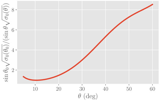
Figure 7.
Relative radial velocity standard deviation referenced to the performance at the SKIM incidence angles, all other parameters being held constant. The penalty in the projection factor is outweighed by the greater brightness at near-nadir incidence.
While reducing the incidence angle has advantages, it also carries disadvantages. Perhaps the largest disadvantage is the reduction in swath width and the associated increase in the observation repeat time for a given location. Although the details of the revisit time as a function of swath-width depends on the details of the orbit selected, we can get a lower bound for the Equatorial revisit time by assuming that the orbit selected is near-polar and ascending and descending tracks are laid out to minimize track overlap at the Equator. In Figure 8, we show the swath width and revisit times as a function of incidence angle assuming a typical sun-synchronous orbit at 700 km altitude. As an example of this trade, we see that the SKIM revisit time (>4 days) is a factor of 4–5 times longer than the revisit time of WaCM (<1 day). When forming time averages, as both missions plan to do, this under-sampling will result in fewer number of independent samples and increased aliasing of fast signals, such as inertial motions.
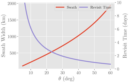
Figure 8.
Swath width (left axis) and revisit time (right axis) as a function of incidence angle.
The second disadvantage is that there is a great residual signature from surface gravity waves at lower incidence angles, which decreases with increasing incidence angle. Ardhuin et al. [7] estimate that the magnitude of this gravity wave contamination at near-nadir incidence can expressed as a wind dependent factor, , which multiplies the Stokes drift magnitude. At Ka-band, G varies between about 15 for high winds and 30 for low winds. As the incidence angle increases and Bragg scattering becomes the dominant scattering mechanism, this multiplicative factor reduces by an order of magnitude and becomes nearly independent of wind speed [13]. In principle, it is possible to remove this wave-induced bias through an empirical or model correction, but it must be removed an order of magnitude more accurately at near-nadir incidence than at higher incidence angles.
The final disadvantage of near-nadir incidence is that in near-nadir incidence, backscatter modulations are mostly governed by wave tilting rather than wind speed; indeed this is the basis for wave spectrometry [8], the architecture from which SKIM is derived. Larger incidence angles, where Bragg scattering applies, are sensitive to wind speed and direction and can be used for wind retrieval [13,19]. Thus, near-nadir incidence is preferable if one prefers to measure waves and currents, while off-nadir angles are preferable when trying to measure surface winds and currents.
4.3. Range Ambiguities and Contiguous Scans
In order to have full imaging without gaps, pencil-beam scanning systems must satisfy two constraints: footprint contiguity and swath continuity. Footprint continuity requires that footprints from subsequent burst are spaced closely enough so that the mapping error from areas that are not imaged is small. In practice, this sets a limit on the Burst Repetition Interval (BRI), which cannot be allowed to grow too large. This sets a limit on the length of bursts that can be transmitted, which, for typical geo-synchronous orbits is in the range between 1 ms to 3 ms, depending on the ocean surface temporal correlation time and the number of bursts in the air, which we assume to be at most 2. In the calculations below, we assume pessimistically, [13], that the ocean correlation time is 1 ms, and this also sets the limit on the performance gain that can be achieved by increasing the BRI in the along-track direction.
A more stringent requirement is swath continuity: the need for scans to leave no holes after each pencil-beam rotation. This requirement places the can be expressed as
where is the number of contiguous range-direction footprints of dimension D that are being used to illuminate the surface, and is the rotation period of the antenna. This requirement often conflicts the requirement that the returns from the desired range footprint does not suffer from range ambiguities (i.e., two locations within the same footprint may arrive at the same time if the PRF is sufficiently high, as in Figure 1). This requirement can be expressed as
where is the Inter-Pulse Period (IPP = 1/PRF), and is the incidence angle. If is fixed by requiring that the broadside region’s Doppler be sampled at Nyquist, or better, this will put a very severe limitation on D. For instance, for SKIM, one has that km, and achieving along-track and footprint continuity cannot be done due to the very high spin rate required. As a consequence, the SKIM error budget [7] includes not only random radial velocity errors, but also mapping errors, which can be of similar magnitude to the random errors and limits the achievable spatial resolution to about 65 km.
As discussed in the sections above, it is better to vary with scan angle as in Equation (29). This will not only improve the radial velocity, as shown in Figure 5, but will also increase the size of the range unambiguous swath:
In Figure 9, we show how this unambiguous swath varies as a function of normalized distance from nadir for a variety of antenna lengths for a system flying at 700 km and imaging at an incidence angle of . Two things can be appreciated from this figure: a longer antenna length increases the range unambiguous swath significantly; and the range unambiguous swath can increase by orders of magnitude away from the broadside direction.
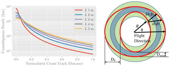
Figure 9.
(Left) Width of the range-PRF unambiguous swath as a function of the normalized cross-track distance from the nadir path. A temporal correlation time of 1 ms is assumed, and fixed antenna area. (Right) Cartoon illustrating the symbols used and showing how ambiguity and overlap requirements vary as a function of flight direction and scan angle. The blue annulus shows the region that has no range ambiguities using the broadside PRF. In green is the area that has no range ambiguities when looking along the flight path. The area enclosed by the red lines shows the area required to be covered to ensure along-track swath continuity.
To take advantage of the variation in range unambiguous swath with scan angle, we advocate using an antenna with a large enough range-direction footprint so that the swath continuity condition can be achieved using one or two scanning beams and vary the PRF with scan angle, as previously discussed. The unambiguous portions of the swath will be small at broadside, but will increase quickly as the scan angle moves away from broadside (see Figure 9). Given the sampling geometry, the need for along-track continuity changes with cross-track distance. It is not difficult to show that along-track continuity for circular annuli requires that one must advance at most in the along-track direction in order to ensure along-track continuity for all cross-track distances:
where R is the inner radius of the annulus, and is the width of the annulus (i.e., the along-track swath). The along-track continuity requirement becomes
which results in a region such as the one between the two red curves in Figure 9 needing to be sampled. This is a much less stringent requirement than the one set by selecting only a single PRF.
4.4. System Spatial Resolution
We have seen in Section 2 that increasing the range bandwidth to the point that the SNR is approximately equal to 1 will yield significant performance benefits. This higher bandwidth is used to gain independent samples, and a range spatial averaging scale should be set when the desired retrieval noise level is achieved. The noise level will reduce by the square root of the number of independent range samples. The azimuth resolution is typically one of the limiting factors of real-aperture scatterometer systems, since it limits coverage near the coasts and contamination by rain cells in the azimuth direction. The azimuth resolution is improved by increasing the antenna length, which also benefits Doppler sampling and spin-rate considerations. An increase in the antenna length by a factor a, will lead to a decrease of the scattering area by , thus lowering the SNR by . On the other hand, for a given final azimuth sampling and assuming continuous azimuth footprints, the number of azimuth independent looks will increase by a. Since the performance in Equation (35) scales as , where is the number of azimuth looks, the combined effect of SNR and azimuth looks for a given azimuth posting will remain constant. We conclude therefore that the antenna size should be set to minimize the Doppler bandwidth, as described above, and enable the desired resolution close to the coasts or of relevant circulation features.
5. Design Examples
In this section we re-examine the WaCM design [6], but assume that different antennas or transmit power could be available. It should be emphasized that the examples in this section are illustrative of performance given typical radar system capabilities, but do not include a detailed design where specific components have been identified. An actual design will likely differ somewhat, but the performance is expected to be of the same order of magnitude.
As a basis for the antenna, we take the 5-m long Ka-band reflectarray antenna that has been developed by the NASA SWOT mission as the longest antenna that could be easily considered with the state of the art. The antenna parameters used for this antenna are representative of the SWOT antenna (R. Hodges, JPL, private communication), but we assume that the antenna width can be increased to 0.35 m, to improve gain and sidelobes and achieve an easier form factor to illuminate. We also assume separate receive and transmit feeds to mitigate scan loss, not encountered in SWOT. To trade antenna length without sacrificing noise-equivalent , we keep the antenna area constant by increasing the width proportionately.
In addition to the antenna length, we also examine the impact from changing transmit power. For WaCM [6], we assumed that a 120 W transmitter was available, since a solid-state transmitter suitable for SWOT had already been developed for NASA’s DopplerScatt [13]. However, higher power is available at Ka-band; for instance, the SWOT mission uses a 1.5 kW EIK. Transmitting this high power with high duty cycle may not be feasible for engineering or cost issues, so we also consider an intermediate case where 400 W peak transmit power is available, probably from a combination of Traveling Wave Tube Amplifiers (TWTA).
The value of dB, corresponding to the maximum likelihood wind speed of 6 m/s is used in all calculations, and the wind speed threshold for evaluating the error over wind speeds is set to 3 m/s. Finally, we select the resolution of the instrument after averaging in range and azimuth to be 5 km, comparable with the SKIM 6 km footprint and the resolution desires of the ocean community [2]. Table 1 summarizes the system and derived parameters, including noise equivalent for the single look, as discussed in Section 2.

Table 1.
System parameters.
We first examine the effect of antenna length, assuming the lowest transmit power, and plot the expected radial velocity errors (projected on the ocean surface) in Figure 10, assuming a conservative ocean correlation time of 1 ms. This figure shows that, even though the longer antenna has a higher noise equivalent , the reduction in Doppler bandwidth clearly makes up for it and produces significantly better performance across the swath. These radial velocity errors can be turned into velocity component errors, following [13]. The results are presented in Figure 11. These should be compared against the [2], where an assumption of 0.5 m/s errors at 5 km resolution was used to show that a system that could deliver this performance would benefit the oceanographic community significantly. The results presented here show that, given a 4–5 m antenna, this type of performance can be exceeded over much of the swath but falls short at the edges. The large antenna length along-track velocity component error satisfies the 0.25 m/s goal stated in [2] for a significant portion of the swath, but the cross-track component has errors on the order of 0.3 m/s for much of the swath.
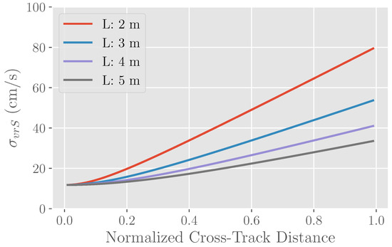
Figure 10.
Surface projected radial velocity error as a function of normalized cross-track distance from nadir for a peak output power of 100 W and varying antenna length, L. This performance assume only one pencil beam.
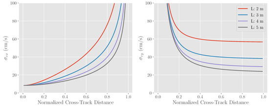
Figure 11.
Expected surface velocity standard deviation as a function of normalized cross-track distance from nadir for the along-track (left) and cross-track (right) surface velocity components for a peak output power of 100 W and varying antenna length, L.
Since it is not realistic to try to increase antenna length much beyond 5 m, I examine next the impact of increasing the transmit power. Figure 12 shows the errors in radial velocity for the two longest antenna lengths and the range of powers discussed above. As expected, improvements are about a factor of 2, given the square root scaling of the performance with power. Figure 13 shows the equivalent performance for the surface velocity components. Clearly, the use of additional power and a long antenna can meet the 0.25 m/s goal set by Chelton et al. [2], while the high-power performance will be below 0.1 m/s for much of the swath.
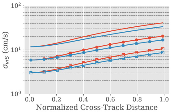
Figure 12.
Surface-projected radial velocity error as a function of normalized cross-track distance from nadir for antenna lengths, L, of 4 m (red) and 5 m (blue) and for peak output power of 100 W (no marker), 400 W (filled circles), 1.5 kW (empty rectangles).
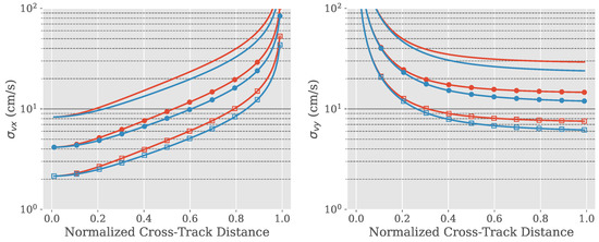
Figure 13.
Expected surface velocity standard deviation as a function of normalized cross-track distance from nadir for the along-track (left) and cross-track (right) surface velocity components for antenna lengths, L, of 4 m (red) and 5 m (blue) and for peak output power of 100 W (no marker), 400 W (filled circles), 1.5 kW (empty rectangles).
6. Conclusions
This paper presented how Doppler scatterometers can be optimized to measure surface winds and currents simultaneously. The following list summarizes the lessons learned from this optimization process:
- The system bandwidth should be chosen so that the signal-to-noise ratio is approximately 1. This somewhat counterintuitive result can be understood as balancing the number of looks and the SNR in the equation, and will typically lead to higher bandwidths than in historical designs (e.g., QuikSCAT).
- Varying the inter-pulse period as a function of scan angle so that the Doppler bandwidth is appropriately sampled (but not over-sampled) can have significant benefits in the radial velocity performance. One should use the opportunity presented by longer pulse correlation times to separate the pulses as much as possible, while lengthening them to improve the SNR per pulse.
- As high a frequency should be chosen as possible, all other things being equal.
- The fast change in brightness with incidence angle strongly suggests that near-nadir incidence angles be used, as in SKIM. However, increasing the antenna length can mitigate this significantly. Near-nadir incidence angles have additional disadvantages in terms of temporal revisit and mapping errors, due to the reduced swath. The incidence angle is probably the parameter that needs most optimization to balance random measurement errors and interpolation mapping errors.
- Varying the PRF has significant advantages for the continuity of the along-track coverage and minimizing range ambiguities.
- It is possible, with systems that are at the present state of the art, to achieve the performance goals outlined by Chelton et al. [2]. A high-power system will exceed these requirements, but may have greater engineering challenges.
The optimal sampling techniques proposed here can be incorporated into any of the point designs described in the introduction [4,5,6,7], as long as the hardware can support it. The following two major improvements can be expected in the performance:
- By varying the spacing between the pulses while keeping the total burst energy constant, one can expect significant improvements (up to an order of magnitude in the along-track direction) for the radial velocity error, as shown in Figure 5.
- By varying the PRF, one can increase substantially (up to two orders of magnitude in the along-track direction) the unambiguous footprint, as shown in Figure 9. This allows ground coverage without gaps with a moderate-sized antenna at antenna realizable spin-rates. This is beneficial in the mission mechanical design.
Funding
This research was funded by National Aeronautics and Space Administration (NASA) grant number NNN13D462T.
Acknowledgments
The research presented in the paper was carried out at the Jet Propulsion Laboratory, California Institute of Technology, under contract with the National Aeronautics and Space Administration. Copyright 2018 California Institute of Technology. U.S. Government sponsorship acknowledged.
Conflicts of Interest
The author declares no conflict of interest.
Appendix A
The minimum of ) is obtained by requiring that the derivatives of with respect to both parameters vanish. This yields the set of equations
Multiplying the first equation by , the second by , and subtracting them, one can solve for as a function of :
Replacing this in the first equation and simplifying leads to the equation
where . This equation can be solved by iteration starting from the initial guess , and converges within one iteration to better than 1% accuracy relative to the solution obtained using Newton’s method. It agrees to 4 significant digits within 5 iterations. The final result is and .
Appendix B
Table A1.
Symbols table order as introduced in text.
Table A1.
Symbols table order as introduced in text.
| Symbol | Description |
|---|---|
| Normalized radar cross section. | |
| Error in parameter x | |
| Coefficient of variation | |
| v | Speed |
| Azimuth angle. | |
| Radial velocity. | |
| Pulse-pair phase. | |
| Radial velocity | |
| EM wavelength | |
| k | EM wavenumber |
| Inter-pulse period. | |
| Standard deviation of parameter x. | |
| Number of range samples. | |
| Number of independent pulse pair samples | |
| Total correlation coefficient. | |
| Thermal noise correlation. | |
| Temporal correlation. | |
| Doppler correlation. | |
| Burst time. | |
| Pulse-pair correlation time. | |
| Water correlation time. | |
| Platform speed | |
| SNR | Signal-to-noise ratio. |
| Noise-to-signal ratio | |
| Gaussian azimuth antenna pattern standard deviation. | |
| L | Antenna length |
| Azimuth beamwidth factor. | |
| B | System bandwidth |
| X | Desired range resolution. |
| Incidence angle | |
| c | Speed of light. |
| Minimum bandwidth | |
| Noise-only minimization function (Equation (20)) | |
| Optimal number of range looks | |
| Optimum | |
| Temporal and noise minimization function (Equation (25)) | |
| Optimal | |
| Optimal | |
| Optimal radial velocity | |
| Most likely wind speed. | |
| s | Wind speed normalized by most likely wind speed. |
| Wind speed probability density function. | |
| for most likely wind speed | |
| Noise-equivalent | |
| for most likely wind speed | |
| relative to most likely wind | |
| Average over wind speeds | |
| Antenna azimuth resolution | |
| Final azimuth resolution after averaging | |
| Number of contiguous range-direction footprints | |
| D | Size of range footprint |
| Rotation period | |
| R | Inner radius of the scanned annulus |
| Width of the annulus (i.e., the along-track swath) | |
| Along-track direction in order to ensure along-track continuity |
References
- The National Academy of Sciences, Engineering, and Medicine. Thriving on Our Changing Planet: A Decadal Strategy for Earth Observation from Space; The National Academy Press: Washington, DC, USA, 2018. [Google Scholar]
- Chelton, D.B.; Schlax, M.G.; Samelson, R.M.; Farrar, J.T.; Molemaker, M.J.; McWilliams, J.C.; Gula, J. Prospects for Future Satellite Estimation of Small-Scale Variability of Ocean Surface Velocity and Vorticity. Prog. Oceanogr. 2018, in press. [Google Scholar] [CrossRef]
- Spencer, M.; Tsai, W.; Long, D. High-Resolution Measurements with a Spaceborne Pencil-Beam Scatterometer Using Combined Range/Doppler Discrimination Techniques. IEEE Trans. Geosci. Remote Rens. 2003, 41, 567–581. [Google Scholar] [CrossRef]
- Bao, Q.; Dong, X.; Zhu, D.; Lang, S.; Xu, X. The Feasibility of Ocean Surface Current Measurement Using Pencil-Beam Rotating Scatterometer. IEEE J. Sel. Top. Appl. Earth Observ. Remote Sens. 2015, 8, 3441–3451. [Google Scholar] [CrossRef]
- Miao, Y.; Dong, X.; Bao, Q.; Zhu, D. Perspective of a Ku-Ka Dual-Frequency Scatterometer for Simultaneous Wide-Swath Ocean Surface Wind and Current Measurement. Remote Sens. 2018, 10, 1042. [Google Scholar] [CrossRef]
- Bourassa, M.; Rodriguez, E.; Chelton, D. Winds and currents mission: Ability to observe mesoscale AIR/SEA coupling. In Proceedings of the 2016 IEEE International Geoscience and Remote Sensing Symposium, Beijing, China, 10–15 July 2016. [Google Scholar]
- Ardhuin, F.; Aksenov, Y.; Benetazzo, A.; Bertino, L.; Brandt, P.; Caubet, E.; Chapron, B.; Collard, F.; Cravatte, S.; Dias, F.; et al. Measuring currents, ice drift, and waves from space: The Sea Surface KInematics Multiscale monitoring (SKIM) concept. Ocean Sci. 2018, 14, 337–354. [Google Scholar] [CrossRef]
- Jackson, F.C.; Walton, T.W.; Baker, P.L. Aircraft and satellite measurement of ocean wave directional spectra using scanning-beam microwave radars. J. Geophys. Res. 1985, 90, 987–1004. [Google Scholar] [CrossRef]
- Gommenginger, C.; Chapron, B.; Martin, A.; Marquez, J.; Brownsword, C.; Buck, C. SEASTAR: A new mission for high-resolution imaging of ocean surface current and wind vectors from space. In Proceedings of the 12th European Conference on Synthetic Aperture Radar, Aachen, Germany, 4–7 June 2018. [Google Scholar]
- Fois, F.; Hoogeboom, P.; Chevalier, F.; Stoffelen, A.; Mouche, A. DopSCAT: A mission concept for simultaneous measurements of marine winds and surface currents. J. Geophys. Res. Oceans 2015, 120, 7857–7879. [Google Scholar] [CrossRef]
- Stoffelen, A.; Aaboe, S.; Calvet, J.C.; Cotton, J.; Chiara, G.; Saldaa, J.; Mouche, A.; Portabella, M.; Scipal, K.; Wagner, W. Scientific Developments and the EPS-SG Scatterometer. IEEE J. Sel. Top. Appl. Earth Observ. Remote Sens. 2017, 10, 2086–2097. [Google Scholar] [CrossRef]
- Hoogeboom, P.; Stoffelen, A.; Lopez Dekker, P. Ocean Current with DopSCA. In Proceedings of the 2018 Doppler Oceanography from Space Symposium, Brest, France, 10–12 October 2018. [Google Scholar]
- Rodriguez, E.; Wineteer, A.; Perkovic-Martin, D.; Gal, T.; Stiles, B.; Niamsuwan, N.; Monje, R. Estimating Ocean Vector Winds and Currents Using a Ka-Band Pencil-Beam Doppler Scatterometer. Remote Sens. 2018, 10, 576. [Google Scholar] [CrossRef]
- Long, D.G.; Spencer, M.W. Radar backscatter measurement accuracy for a spaceborne pencil-beam wind scatterometer with transmit modulation. IEEE Trans. Geosci. Remote Sens. 1997, 35, 102–114. [Google Scholar] [CrossRef]
- Spencer, M.W.; Wu, C.; Long, D.G. Tradeoffs in the design of a spaceborne scanning pencil beam scatterometer: Application to SeaWinds. IEEE Trans. Geosci. Remote Sens. 1997, 35, 115–126. [Google Scholar] [CrossRef]
- Oliphant, T.E.; Long, D.G. Accuracy of scatterometer-derived winds using the Cramer-Rao bound. IEEE Trans. Geosci. Remote Sens. 1999, 37, 2642–2652. [Google Scholar] [CrossRef]
- Wentz, F.; Smith, D. A model function for the ocean-normalized radar cross section at 14 GHz derived from NSCAT observations. J. Geophys. Res. Oceans 1999, 104, 11499–11514. [Google Scholar] [CrossRef]
- Ricciardulli, L.; Wentz, F. A Scatterometer Geophysical Model Function for Climate-Quality Winds: QuikSCAT Ku-2011. J. Atmos. Ocean. Technol. 2015, 32, 1829–1846. [Google Scholar] [CrossRef]
- Yurovsky, Y.; Kudryavtsev, V.N.; Grodsky, S.A.; Chapron, B. Ka-Band Dual Copolarized Empirical Model for the Sea Surface Radar Cross Section. IEEE Geosci. Remote Sens. 2016, 55, 1629–1647. [Google Scholar] [CrossRef]
- Spencer, M.; Wu, C.; Long, D. Improved Resolution Backscatter Measurements with the SeaWinds Pencil-Beam Scatterometer. IEEE Trans. Geosci. Remote Sens. 2000, 38, 89–104. [Google Scholar] [CrossRef]
- Freilich, M.; Challenor, P. A New Approach for Determining Fully Empirical Altimeter Wind Speed Model Functions. J. Geophys. Res. Oceans 1994, 99, 25051–25062. [Google Scholar] [CrossRef]
- Shankaranarayanan, K.; Donelan, M. A probabilistic approach to scatterometer model function verification. J. Geophys. Res. Oceans 2001, 106, 19969–19990. [Google Scholar] [CrossRef]
© 2018 by the author. Licensee MDPI, Basel, Switzerland. This article is an open access article distributed under the terms and conditions of the Creative Commons Attribution (CC BY) license (http://creativecommons.org/licenses/by/4.0/).