Relationship between Spatiotemporal Variations of Climate, Snow Cover and Plant Phenology over the Alps—An Earth Observation-Based Analysis

 , ,
, , 
Abstract
1. Introduction
- Which patterns show the temporal and spatial variabilities of snow and vegetation phenology in dependency of topography and land cover over the Alps?
- Can statistical relationships between vegetation phenology and snow cover be detected in dependency of the altitude? Are there time lags?
- What is the common seasonality between vegetation phenology, snow, and climate parameters? Which parameters are most important in which altitude? Are there time lags?
- Is there a combined influence of climate parameters and snow on phenology?
2. Materials and Methods
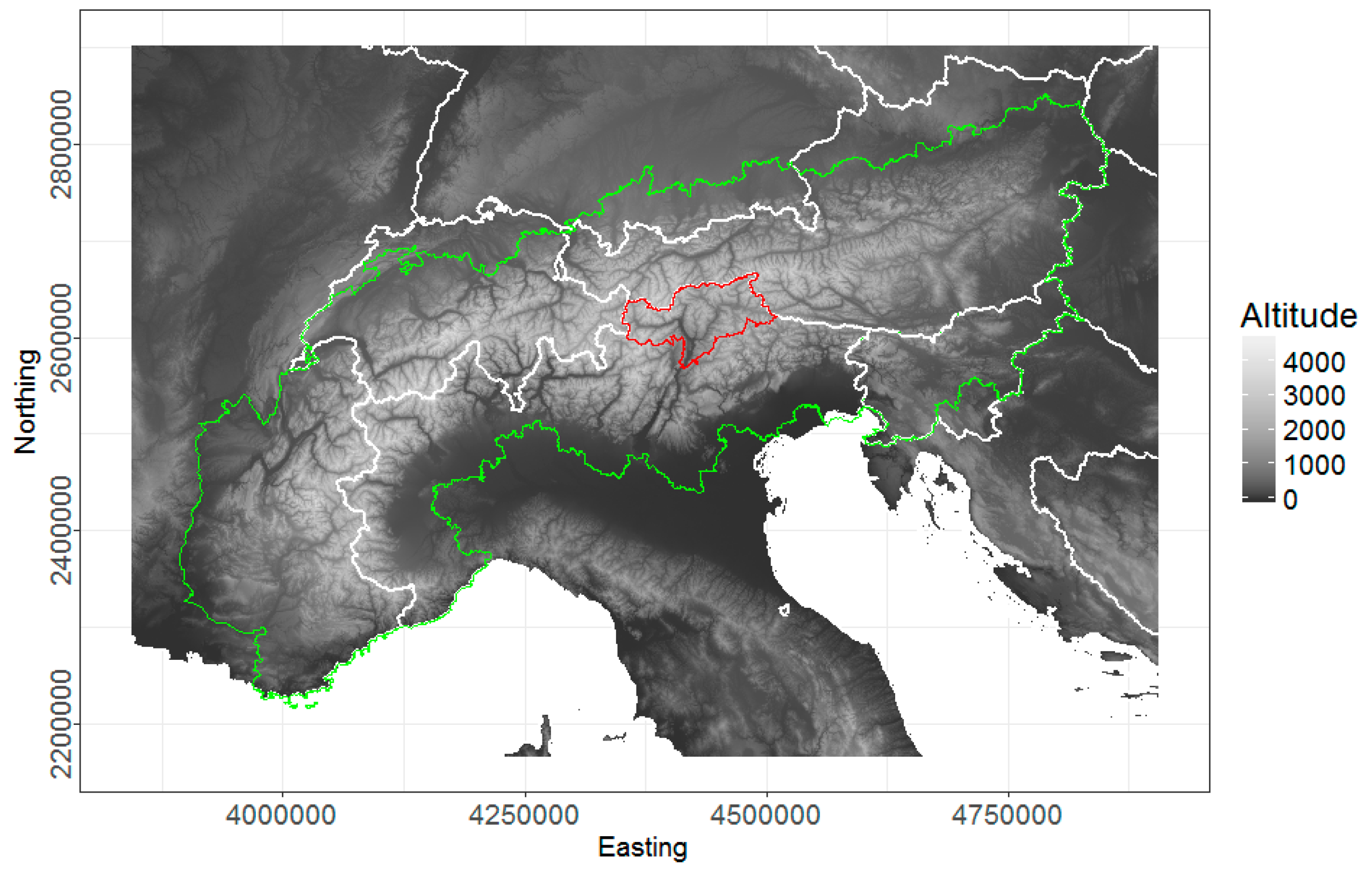
2.1. Study Area
2.2. Data
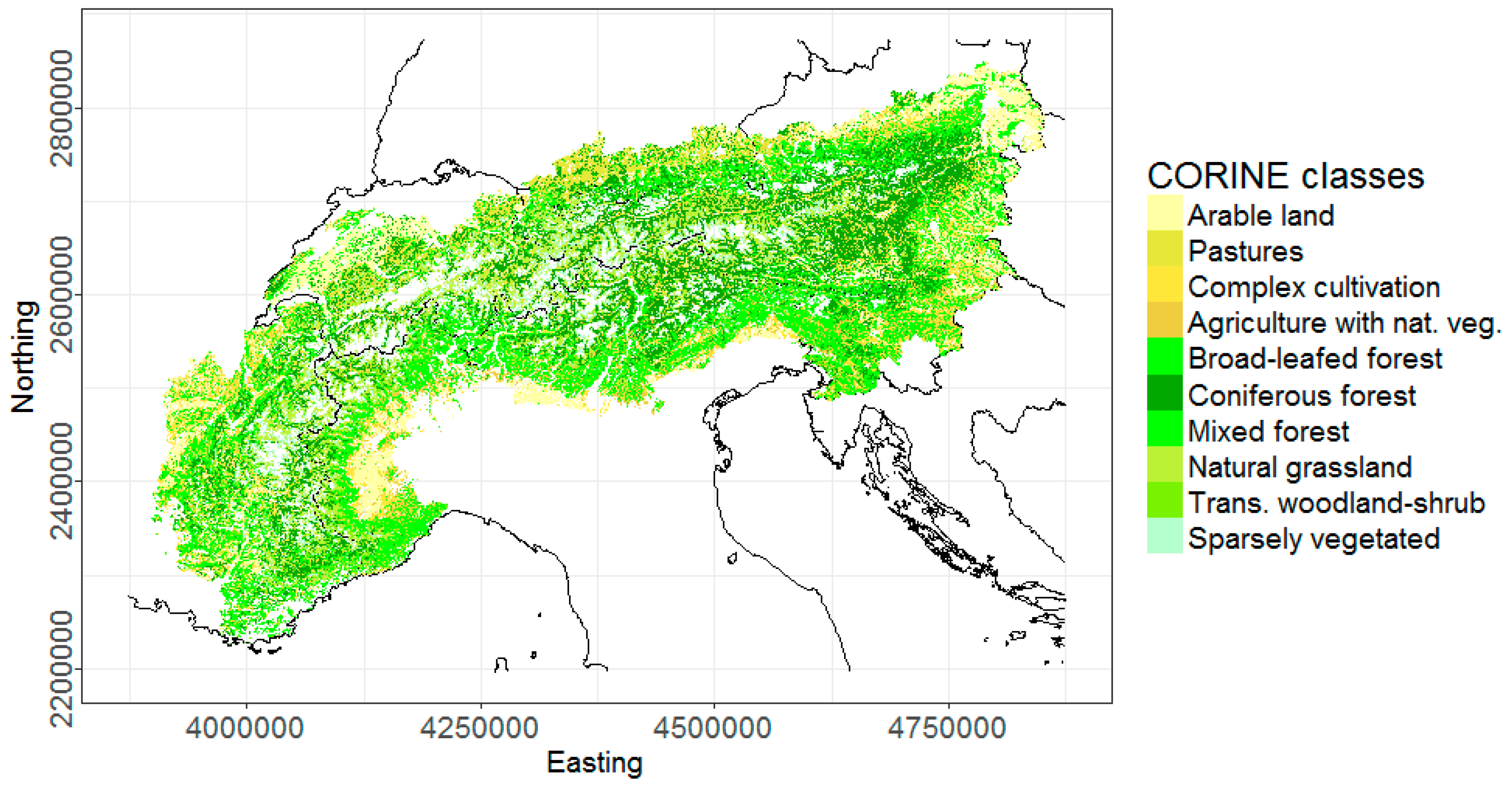
2.2.1. Elevation and Land Cover Data
2.2.2. Snow Data
2.2.3. Vegetation Time Series
2.2.4. Phenology Modeling and Monthly Mean NDVIs
2.2.5. Climate Data
2.3. Statistical Analysis
2.3.1. Analysis on Altitudinal and Temporal Variability of Vegetation Metrics and Snow Cover
2.3.2. Pixel-Wise Correlations between NDVI and SCD
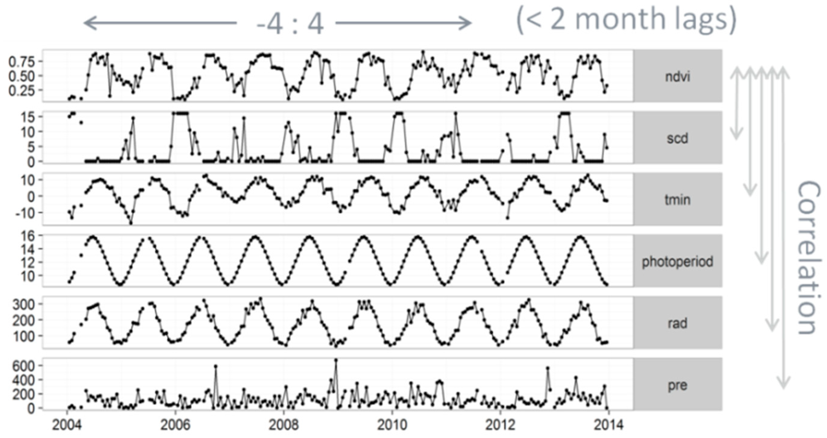
2.3.3. Common Seasonality and Time-Lags of NDVI, Snow and Climatic Drivers
2.3.4. Combined Effects of Snow and Climatic Drivers on NDVI
3. Results
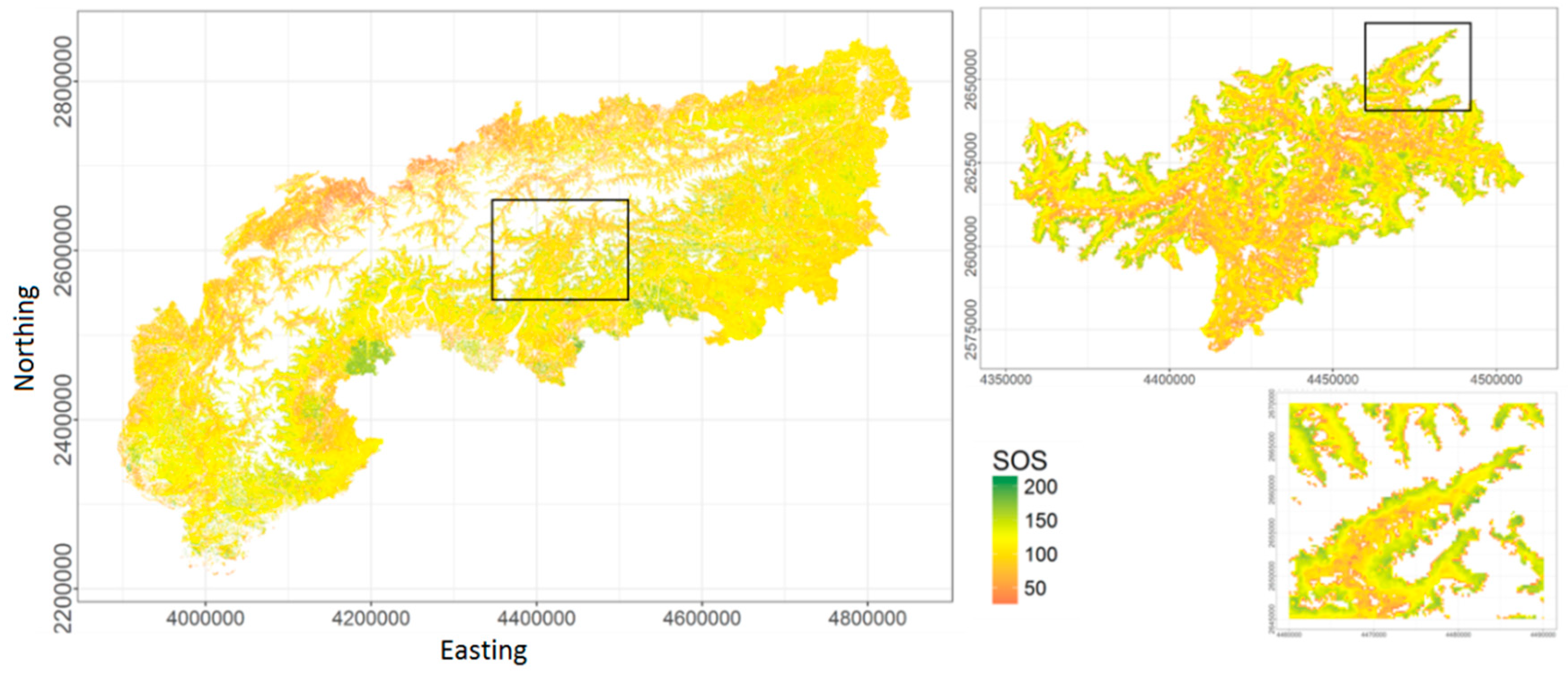
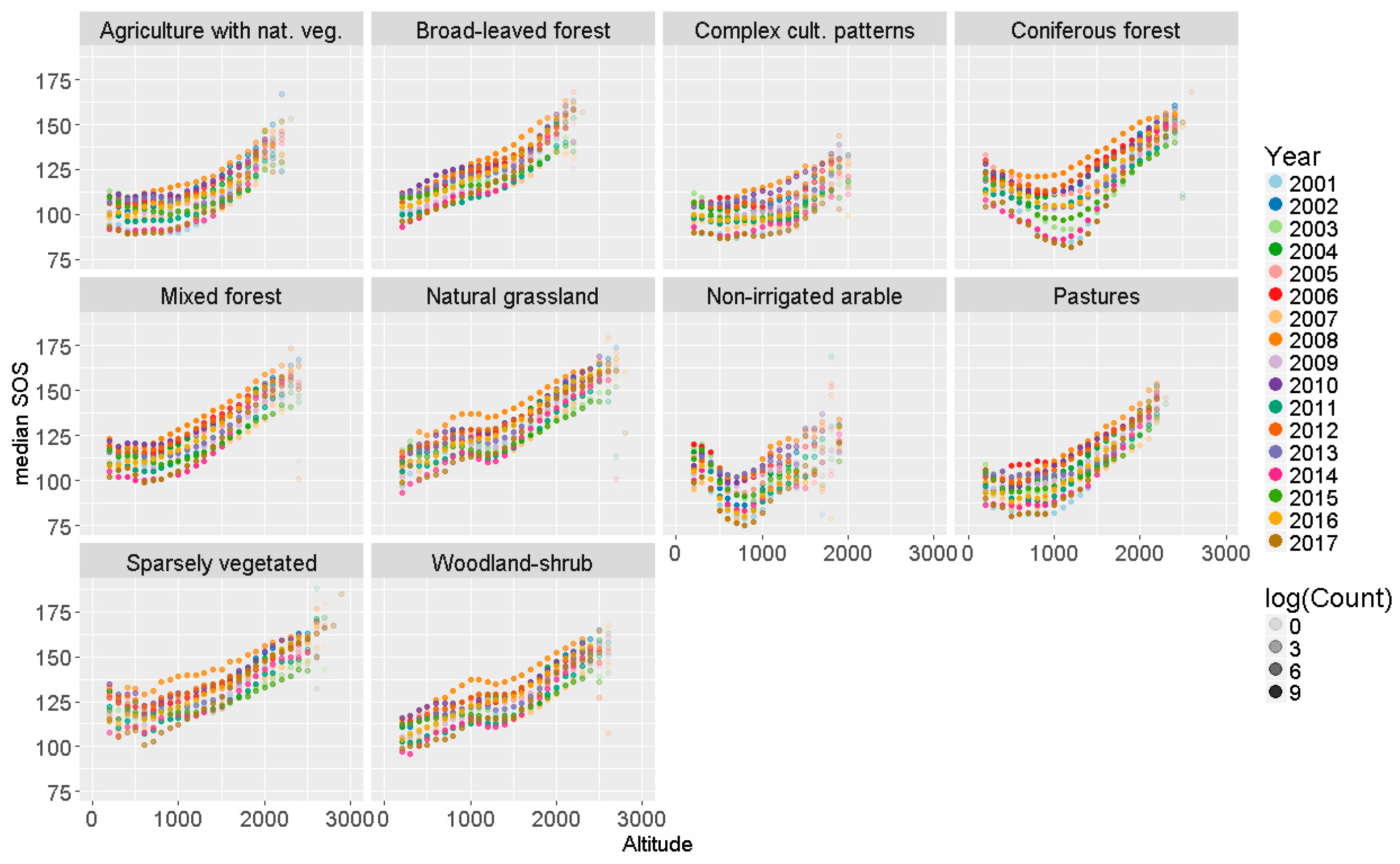
3.1. Temporal and Spatial Variabilities of Vegetation Phenology and Snow Metrics
3.1.1. Vegetation
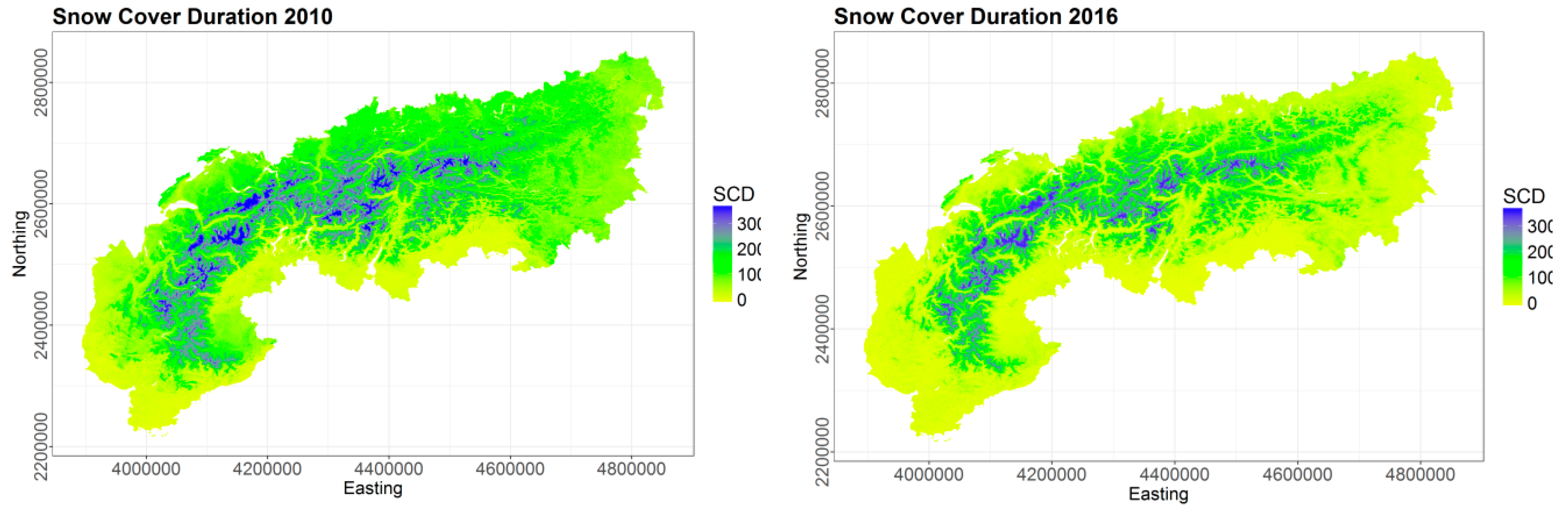
3.1.2. Snow
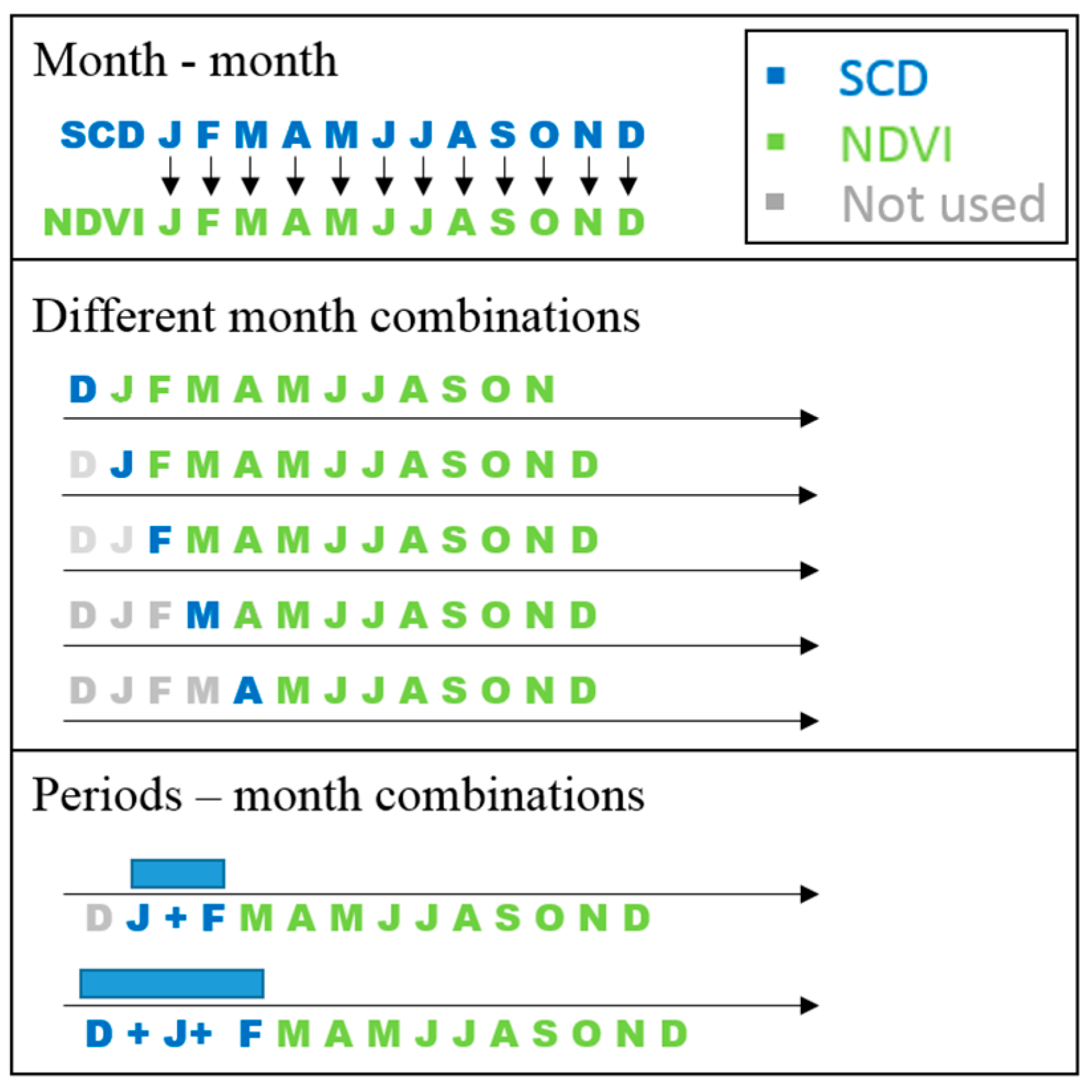
3.2. Inter-Annual Relationship between Monthly SCD and Mean NDVI
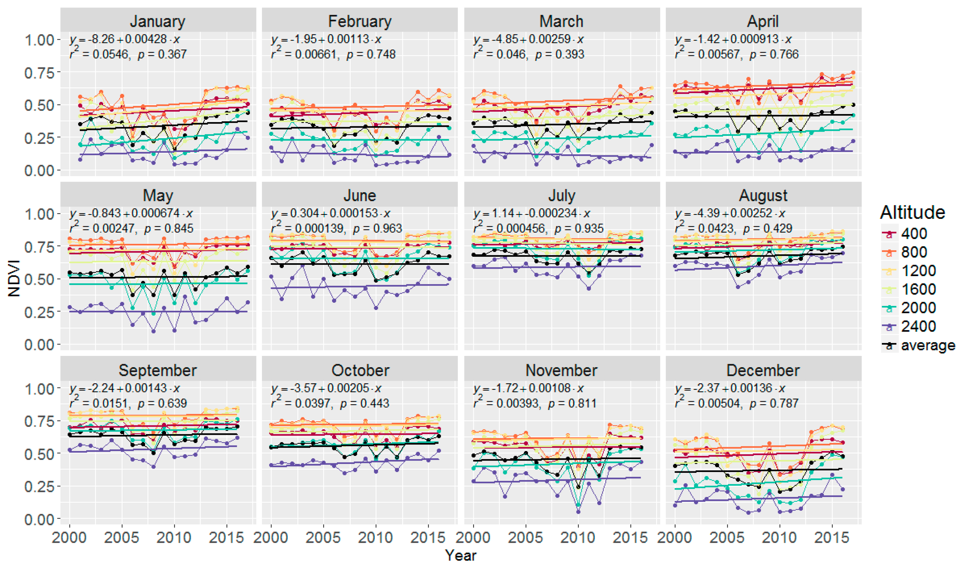
3.3. Intra-Annual Relationships: Common Seasonality of Vegetation Activity and Climate
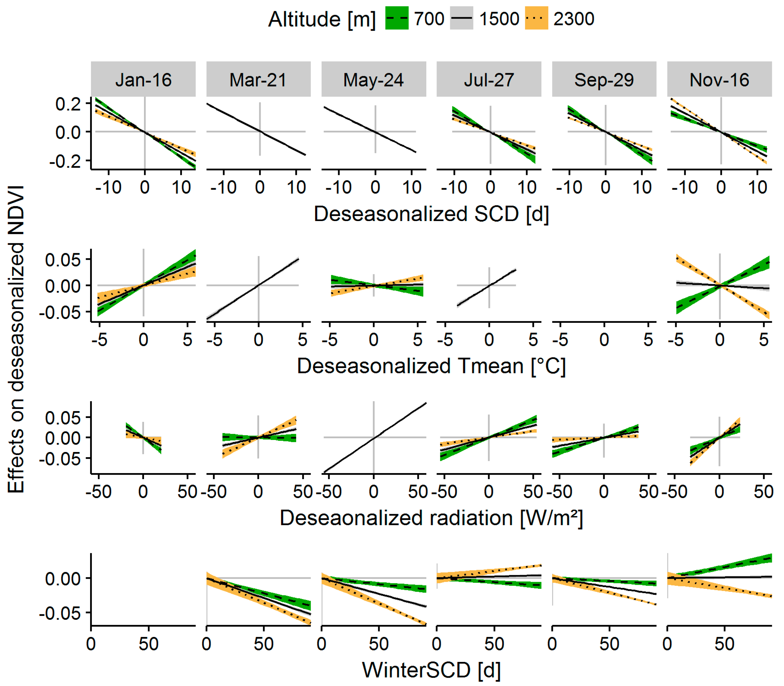
3.4. Combined Effects of Climate Variability on Vegetation Activity Variability
4. Discussion
4.1. Assessment of Spatiotemporal Patterns of Snow and Vegetation Phenology Variability
4.2. Derivation of Statistical Relationships between Vegetation Phenology and Snow Cover
4.3. Assessment of the Common Seasonality and Combined Influence of Climate Parameters and Snow on Phenology
5. Conclusions
Supplementary Materials
Author Contributions
Funding
Acknowledgments
Conflicts of Interest
References
- Jarvis, P.G. The interpretation of the variations in leaf water potential and stomatal conductance found in canopies in the field. Philos. Trans. R. Soc. Lond. B 1976, 273, 593–610. [Google Scholar] [CrossRef]
- Larcher, W. Physiological Plant Ecology: Ecophysiology and Stress Physiology of Functional Groups, 4th ed.; Springer: Heidelberg, Germany, 2003; ISBN 978-3-540-43516-7. [Google Scholar]
- Scheifinger, H.; Menzel, A.; Koch, E.; Peter, C.; Ahas, R. Atmospheric mechanisms governing the spatial and temporal variability of phenological phases in central Europe. Int. J. Climatol. 2002, 22, 1739–1755. [Google Scholar] [CrossRef]
- Menzel, A. Trends in phenological phases in Europe between 1951 and 1996. Int. J. Biometeorol. 2000, 44, 76–81. [Google Scholar] [CrossRef] [PubMed]
- Menzel, A.; Fabian, P. Growing season extended in Europe. Nature 1999, 397, 659. [Google Scholar] [CrossRef]
- Van Vliet, A.J.H.; de Groot, R.S.; Bellens, Y.; Braun, P.; Bruegger, R.; Bruns, E.; Clevers, J.; Estreguil, C.; Flechsig, M.; Jeanneret, F.; et al. The European Phenology Network. Int. J. Biometeorol. 2003, 47, 202–212. [Google Scholar] [CrossRef] [PubMed]
- Betancourt, J.L.; Schwartz, M.D.; Breshears, D.D.; Cayan, D.R.; Dettinger, M.D.; Inouye, D.W.; Post, E.; Reed, B.C. Implementing a U.S. National Phenology Network. Eos Trans. AGU 2005, 86, 539. [Google Scholar] [CrossRef]
- Menzel, A. European phenological response to climate change matches the warming pattern. Glob. Chang. Biol. 2006, 12, 1969–1976. [Google Scholar] [CrossRef]
- Schwartz, M.D.; Reed, B.C.; White, M.A. Assessing satellite derived start-of-season measures in the conterminous USA. Int. J. Climatol. 2002, 22, 1793–1805. [Google Scholar] [CrossRef]
- Fisher, J.I.; Mustard, J.F.; Vadeboncoeur, M.A. Green leaf phenology at Landsat resolution: Scaling from the field to the satellite. Remote Sens. Environ. 2006, 100, 265–279. [Google Scholar] [CrossRef]
- Dunn, A.; de Beurs, K. Land surface phenology of North American mountain environments using moderate resolution imaging spectroradiometer data. Remote Sens. Environ. 2011, 115, 1220–1233. [Google Scholar] [CrossRef]
- Gonsamo, A.; Chen, J.M.; Price, D.T.; Kurz, W.A.; Wu, C. Land surface phenology from optical satellite measurement and CO2 eddy covariance technique. J. Geophys. Res. 2012, 117, G03032. [Google Scholar] [CrossRef]
- Delbart, N.E.; Beaubien, L.; Kergoat, T.; Toan, L. Comparing land surface phenology with leafing and flowering observations from the PlantWatch citizen network. Remote Sens. Environ. 2015, 160, 273–280. [Google Scholar] [CrossRef]
- Garonna, I.; de Jong, R.; Schaepman, M.E. Variability and evolution of global land surface phenology over the past three decades (1982–2012). Glob. Chang. Biol. 2016, 22, 1456–1468. [Google Scholar] [CrossRef] [PubMed]
- Ganguly, S.; Friedl, M.; Tan, A.B.; Zhang, X.; Verma, M. Land surface phenology from MODIS: Characterization of the Collection 5 global land cover dynamics product. Remote Sens. Environ. 2010, 114, 1805–1816. [Google Scholar] [CrossRef]
- De Beurs, K.M.; Henebry, G.M. Spatio-Temporal Statistical Methods for Modelling Land Surface Phenology. In Phenological Research; Springer: Dordrecht, The Netherlands, 2010; pp. 177–208. [Google Scholar]
- White, M.A.; Nemani, R. Real-time monitoring and short-term forecasting of land surface phenology. Remote Sens. Environ. 2006, 104, 43–49. [Google Scholar] [CrossRef]
- Kathuroju, N.; White, M.; Symanzik, J.; Schwartz, M.; Powell, J.; Nemani, R. On the use of the Advanced Very High Resolution Radiometer for development of prognostic land surface phenology models. Ecol. Model. 2007, 201, 144–156. [Google Scholar] [CrossRef]
- Stöckli, R.; Vidale, P.L. European plant phenology and climate as seen in a 20 year AVHRR land-surface parameter dataset. Int. J. Remote Sens. 2004, 25, 3303–3330. [Google Scholar] [CrossRef]
- Studer, S.; Stöckli, R.; Appenzeller, C.; Vidale, P.L. A comparative study of satellite and ground-based phenology. Int. J. Biometeorol. 2007, 51, 405–414. [Google Scholar] [CrossRef] [PubMed]
- Defila, C.; Clot, B. Phytophenological trends in Switzerland. Int. J. Biometeorol. 2001, 45, 203–207. [Google Scholar] [CrossRef] [PubMed]
- Cleland, E.; Chuine, I.; Menzel, A.; Mooney, H.; Schwartz, M. Shifting plant phenology in response to global change. Trends Ecol. Evol. 2007, 22, 357–365. [Google Scholar] [CrossRef] [PubMed]
- Parmesan, C.; Yohe, G. A globally coherent fingerprint of climate change impacts across natural systems. Nature 2003, 421, 37–42. [Google Scholar] [CrossRef] [PubMed]
- Root, T.; Price, J.; Hall, K.; Schneider, S.; Rosenzweig, C.; Pounds, J. Fingerprints of global warming on wild animals and plants. Nature 2003, 421, 57–60. [Google Scholar] [CrossRef] [PubMed]
- Rosenzweig, C.; Casassa, G.; Karoly, D.; Imeson, A.; Liu, C.; Menzel, A.; Rawlins, S.; Root, T.; Seguin, B.; Tryjanowski, P. Assessment of observed changes and responses in natural and managed systems. In Climate Change 2007: Impacts, Adaptation and Vulnerability. Contribution of Working Group II to the Fourth Assessment Report of the Intergovernmental Panel on Climate Change; Cambridge University Press: Cambridge, UK, 2007; pp. 79–131. [Google Scholar]
- Tsvetsinskaya, E.A.; Mearns, L.O.; Easterling, W.E. Investigating the effect of seasonal plant growth and development in threedimensional atmospheric simulations. Part I: Simulation of surface fluxes over the growing season. J. Climatol. 2001, 14, 692–709. [Google Scholar] [CrossRef]
- Lu, P.; Shuttleworth, W.J. Incorporating NDVI-derived LAI into the climate version of rams and its impacts on regional climate. J. Hydrometeorol. 2002, 3, 347–362. [Google Scholar] [CrossRef]
- Kim, Y.; Wang, G.L. Modeling seasonal vegetation variation and its validation against Moderate Resolution Imaging spectroradiometer (MODIS) observations over North America. J. Geophys. Res. 2005, 110, D04106. [Google Scholar] [CrossRef]
- Richardson, A.D.; Keenan, A.D.; Migliavacca, M.; Ryu, Y.; Sonnentag, O.; Toomey, M. Climate change, phenology, and phenological control of vegetation feedbacks to the climate system. Agric. For. Meteorol. 2013, 169, 156–173. [Google Scholar] [CrossRef]
- Stöckli, R.; Rutishauser, T.; Dragoni, D.; O’Keefe, J.; Thornton, P.E.; Jolly, M.; Lu, L.; Denning, A.S. Remote sensing data assimilation for a prognostic phenology model. J. Geophys. Res. 2008, 113, G04021. [Google Scholar] [CrossRef]
- Buermann, W.; Dong, J.R.; Zeng, X.B.; Myneni, R.B.; Dickinson, R.E. Evaluation of the utility of satellite-based vegetation leaf area index data for climate simulations. J. Clim. 2001, 14, 3536–3550. [Google Scholar] [CrossRef]
- Lawrence, D.M.; Slingo, J.M. An annual cycle of vegetation in a GCM. Part I: Implementation and impact on evaporation. Clim. Dyn. 2004, 22, 87–105. [Google Scholar] [CrossRef]
- Foley, J.A.; Prentice, J.A.; Ramankutty, N.; Levis, S.; Pollard, D.; Sitch, S.; Haxeltine, A. An integrated biosphere model of land surface processes, terrestrial carbon balance, and vegetation dynamics. Glob. Biogeochem. Cycles 1996, 10, 603–628. [Google Scholar] [CrossRef]
- Sellers, P.J.; Los, S.O.; Tucker, C.J.; Justice, C.O.; Dazlich, D.A.; Collatz, G.J.; Randall, D.A. A revised land surface parameterization (SiB2) for atmospheric GCMs. 2. The generation of global fields of terrestrial biophysical parameters from satellite data. J. Climatol. 1996, 9, 706–737. [Google Scholar] [CrossRef]
- Chuine, I. A unified model for budburst of trees. J. Theor. Biol. 2000, 207, 337–347. [Google Scholar] [CrossRef] [PubMed]
- Cox, P.M. Description of the TRIFFID Dynamic Global Vegetation Model; Tech. Rep. 24; Hadley Center: Bracknell, UK, 2001. [Google Scholar]
- Levis, S.; Bonan, G.B.; Vertenstein, M.; Oleson, K.W. The Community Land Model’s Dynamic Global Vegetation Model (CLM-DGVM), Technical Description and User’s Guide; NCAR Technical Note NCAR/TN-459+IA; NCAR: Boulder, CO, USA, 2004. [Google Scholar]
- Jolly, W.M.; Nemani, R.; Running, S. A generalized, bioclimatic index to predict foliar phenology in response to climate. Glob. Chang. Biol. 2005, 11, 619–632. [Google Scholar] [CrossRef]
- Arora, V.K.; Boer, G.J. A parameterization of leaf phenology for the terrestrial ecosystem component of climate models. Glob. Chang. Biol. 2005, 11, 39–59. [Google Scholar] [CrossRef]
- Gibelin, A.L.; Calvet, J.C.; Roujean, J.L.; Jarlan, L.; Los, S.O. Ability of the land surface model ISBA-A-gs to simulate leaf area index at the global scale: Comparison with satellites products. J. Geophys. Res. 2006, 111, D18102. [Google Scholar] [CrossRef]
- Dickinson, R.E.; Tian, Y.; Liu, Q.; Zhou, L. Dynamics of leaf area for climate and weather models. J. Geophys. Res. 2008, 113, D16115. [Google Scholar] [CrossRef]
- White, M.; Thornton, P.E.; Running, S.W. A continental phenology model for monitoring vegetation responses to interannual climatic variability, Global Biogeochem. Cycles 1997, 11, 217–234. [Google Scholar] [CrossRef]
- Barry, R. Past and potential changes in mountain environments: A review. In Mountain Environments in Changing Climates; Routledge: London, UK, 1994; pp. 3–33. [Google Scholar]
- Beniston, M.; Diaz, H.; Bradley, R. Climatic change at high elevation sites: An overview. Clim. Chang. 1997, 36, 233–251. [Google Scholar] [CrossRef]
- Wanner, H.; Rickli, R.; Salvisberg, E.; Schmutz, C.; Schuepp, M. Global climate change and variability and its influence on Alpine climate—Concepts and observations. Theor. Appl. Climatol. 1997, 58, 221–243. [Google Scholar] [CrossRef]
- Chersich, S.; Rejšek, K.; Vranová, V.; Bordoni, M.; Meisina, C. Climate change impacts on the Alpine ecosystem: An overview with focus on the soil—A review. J. For. Sci. 2015, 61, 496–514. [Google Scholar] [CrossRef]
- Theurillat, J.-P.; Guisan, A. Potential impact of climate change on vegetation in the European Alps: A review. Clim. Chang. 2001, 50, 77–109. [Google Scholar] [CrossRef]
- Gobiet, A.; Kotlarski, S.; Beniston, M.; Heinrich, G.; Rajczak, J.; Stoffel, M. 21st century climate change in the European Alps—A review. Sci. Total Environ. 2014, 493, 1138–1151. [Google Scholar] [CrossRef] [PubMed]
- Pepin, N.; Bradley, R.S.; Diaz, H.F.; Baraer, M.; Caceres, E.B.; Forsythe, N.; Fowler, H.; Greenwood, G.; Hashmi, M.Z.; Liu, X.D.; et al. Elevation-dependent warming in mountain regions of the world. Nat. Clim. Chang. 2015, 5, 424–430. [Google Scholar] [CrossRef]
- Palazzi, E.; Mortarini, L.; Terzago, S.; von Hardenberg, J. Elevation-dependent warming in global climate model simulations at high spatial resolution. Clim. Dyn. 2018, 1–18. [Google Scholar] [CrossRef]
- Grabherr, G.; Gottfried, M.; Pauli, H. Climate effects on mountain plants. Nature 1994, 369, 448. [Google Scholar] [CrossRef] [PubMed]
- Walther, G.R.; Beissner, S.; Burga, C. Trends in the upward shift of alpine plants. J. Veg. Sci. 2005, 16, 541–548. [Google Scholar] [CrossRef]
- Steinbauer, M.; Grytnes, J.; Jurasinski, G.; Kulonen, A.; Lenoir, J.; Pauli, H.; Rixen, C.; Winkler, M.; Bardy-Durchhalter, M.; Barni, E.; et al. Accelerated increase in plant species richness on mountain summits is linked to warming. Nature 2018, 556, 231–234. [Google Scholar] [CrossRef] [PubMed]
- Lenoir, J.; Gégout, J.C.; Marquet, P.A.; de Ruffray, P.; Brisse, H. A significant upward shift in plant species optimum elevation during the 20th century. Science 2008, 230, 1768–1771. [Google Scholar] [CrossRef] [PubMed]
- Pauli, H.; Gottfried, M.; Dullinger, S.; Abdaladze, O.; Akhalkatsi, M.; Alonso, J.L.B.; Coldea, G.; Dick, J.; Erschbamer, B.; Calzado, R.F.; et al. Recent plant diversity changes on Europe’s mountain summits. Science 2012, 336, 353–355. [Google Scholar] [CrossRef] [PubMed]
- Gottfried, M.; Pauli, H.; Futschik, A.; Akhalkatsi, M.; Barančok, P.; Benito Alonso, J.; Coldea, G.; Dick, J.; Erschbamer, B.; Fernández Calzado, M.; et al. Continent-wide response of mountain vegetation to climate change. Nat. Clim. Chang. 2012, 2, 111–115. [Google Scholar] [CrossRef]
- Dullinger, S.; Gattringer, A.; Thuiller, W.; Moser, D.; Zimmermann, N.; Guisan, A.; Willner, W.; Plutzar, C.; Leitner, M.; Mang, T.; et al. Extinction debt of high-mountain plants under twenty-first-century climate change. Nat. Clim. Chang. 2012, 2, 619–622. [Google Scholar] [CrossRef]
- Cotto, O.; Wessely, J.; Georges, D.; Klonner, G.; Schmid, M.; Dullinger, S.; Thuiller, W.; Guillaume, F. A dynamic eco-evolutionary model predicts slow response of alpine plants to climate warming. Nat. Commun. 2017, 15399. [Google Scholar] [CrossRef] [PubMed]
- Blois, J.L.; Williams, J.W.; Fitzpatrick, M.C.; Jackson, S.T.; Ferrier, S. Space can substitute for time in predicting climate-change effects on biodiversity. Proc. Natl. Acad. Sci. USA 2013, 110, 9374–9379. [Google Scholar] [CrossRef] [PubMed]
- Fontana, F.; Rixen, C.; Jonas, T.; Aberegg, G.; Wunderle, S. Alpine grassland phenology as seen in AVHRR, VEGETATION, and MODIS NDVI time series—A comparison with in situ measurements. Sensors 2008, 8, 2833–2853. [Google Scholar] [CrossRef] [PubMed]
- Busetto, L.; Colombo, R.; Migliavacca, M.; Cremonese, E.; Meroni, M.; Galvagno, M.; Rossini, M.; Siniscalco, C.; Morra di Cella, U.; Pari, E. Remote sensing of larch phenological cycle and analysis of relationships with climate in the Alpine region. Glob. Chang. Biol. 2010, 2504–2517. [Google Scholar] [CrossRef]
- Colombo, R.; Busetto, L.; Fava, F.; Di Mauro, B.; Migliavacca, M.; Cremonese, E.; Galvagno, M.; Rossini, M.; Meroni, M.; Cogliati, S.; et al. Phenological monitoring of grassland and larch in the Alps from Terra and Aqua MODIS images. Rivista Italiana di Telerilevamento 2011, 43, 83–96. [Google Scholar] [CrossRef]
- Colombo, R.; Busetto, L.; Migliavacca, M.; Cremonese, E.; Meroni, M.; Galvagno, M.; Rossini, M.; Siniscalco, C.; Morra di Cella, U. On the spatial and temporal variability of Larch phenological cycle in mountainous areas. Rivista Italiana di Telerilevamento 2009, 41, 79–96. [Google Scholar] [CrossRef]
- Choler, P. Growth response of temperate mountain grasslands to inter-annual variations in snow cover duration. Biogeosciences 2015, 12, 3885–3897. [Google Scholar] [CrossRef]
- Jolly, W.M.; Dobbertin, M.; Zimmermann, N.E.; Reichstein, M. Divergent vegetation growth responses to the 2003 heat wave in the Swiss Alps. Geophys. Res. Lett. 2005, 32, L18409. [Google Scholar] [CrossRef]
- Reichstein, M.; Ciais, P.; Papale, D.; Valentini, R.; Running, S.; Viovy, N.; Cramer, W.; Granier, A.; Ogee, J.; Allard, V.; Aubinet, M.; et al. Reduction of ecosystem productivity and respiration during the European summer 2003 climate anomaly: A joint flux tower, remote sensing and modelling analysis. Glob. Chang. Biol. 2007, 13, 634–651. [Google Scholar] [CrossRef]
- Auer, I.; Böhm, R.; Jurkovic, A.; Lipa, W.; Orlik, A. HISTALP—Historical instrumental climatological surface time series of the Greater Alpine Region. Int. J. Climatol. 2007, 27, 17–46. [Google Scholar] [CrossRef]
- Inouye, D.; Wielgolaski, F. High altitude climates. In Phenology: An Integrative Environmental Science; Kluwer Academic Publisher: Dordrecht, The Netherlands, 2003. [Google Scholar]
- Kulonen, A.; Imboden, R.; Rixen, C.; Maier, S.; Wipf, S. Enough space in a warmer world? Microhabitat diversity and small-scale distribution of alpine plants on mountain summits. Divers. Distrib. 2018, 24, 252–261. [Google Scholar] [CrossRef]
- Myneni, R.; Maggion, S.; Iaquinta, J.; Privette, J.; Gobron, N.; Pinty, B.; Kimes, D.; Verstraete, M.; Williams, D. Optical remote sensing of vegetation: Modeling, caveats, and algorithms. Remote Sens. Environ. 2008, 51, 169–188. [Google Scholar] [CrossRef]
- Körner, C. The green cover of mountains in a changing environment. In Global Change and Mountain Regions: An Overview of Current Knowledge; Springer: Dordrecht, The Netherlands, 2005; pp. 367–376. [Google Scholar]
- Thompson, J.A. A Remote Sensing Exploration of Land Surface Phenology in the Australian Alps. Ph.D. Thesis, University of Colorado, Denver, CO, USA, 2013. [Google Scholar]
- Wang, K.; Zhang, L.; Qiu, Y.; Ji, L.; Tian, F.; Wang, C.; Wang, Z. Snow effects on alpine vegetation in the Qinghai-Tibetan Plateau. Int. J. Digit. Earth 2013, 1–18. [Google Scholar] [CrossRef]
- Xie, J.; Kneubühler, M.; Garonna, I.; de Jong, R.; Notarnicola, C.; De Gregorio, L.; Schaepman, M.E. Relative Influence of Timing and Accumulation of Snow on Alpine Land Surface Phenology. Biogeosciences 2018, 123, 561–576. [Google Scholar] [CrossRef]
- Isotta, F.A.; Frei, C.; Weilguni, V.; Tadić, M.P.; Lassègues, P.; Rudolf, B.; Pavan, V.; Cacciamani, C.; Antolini, G.; Ratto, S.M.; et al. The climate of daily precipitation in the Alps: Development and analysis of a high-resolution grid dataset from pan-Alpine rain-gauge data. Int. J. Climatol. 2014, 34, 1657–1675. [Google Scholar] [CrossRef]
- Schär, C.; Davies, T.D.; Frei, C.; Wanner, H.; Widmann, M.; Wild, M.; Davies, H. Current alpine climate. In Views from the Alps: Regional Perspectives on Climate Change; MIT Press: Cambridge, MA, USA, 1998. [Google Scholar]
- Directorate-General for Environment. Natura 2000 Nella Regione Alpina. 2010. Available online: http://ec.europa.eu/environment/nature/info/pubs/docs/biogeos/Alpine/KH7809637ITC_002.pdf (accessed on 6 November 2018).
- European Environmental Agency. Regional Climate Change and Adaptation: The Alps Facing the Challenge of Changing Water Resources; EEA Report No. 8/2009; European Environmental Agency: Copenhagen, Denmark, 2009. [Google Scholar]
- Alpine Convention. The Alps in 25 Maps; The Permanent Secretary of the Alpine Convention: Bolzano, Italy, 2018. [Google Scholar]
- Carturan, L.; Filippi, R.; Seooi, R.; Gabrielli, P.; Notarnicola, C.; Bertoldi, L.; Rastner, P.; Cazorzi, F.; Dinale, R.; Fontana, D.G. Area and volume loss of the glaciers in the Ortles-Cevedale group (Eastern Italian Alps): Controls and imbalance of the remaining glaciers. Cryosphere 2013, 1339–1359. [Google Scholar] [CrossRef]
- Bartaletti, F. Geografia e Cultura Delle Alpi; FrancoAngeli: Milan, Italy, 2004; Volume 73. [Google Scholar]
- Jarvis, A.; Reuter, H.; Nelson, A.; Guevara, E. Hole-Filled SRTM for the Globe Version 4. 2008. Available online: http://srtm.csi.cgiar.org (accessed on 6 November 2018).
- McCune, B.; Keon, D. Equations for potential annual direct incident radiation and heat load. J. Veg. Sci. 2002, 13, 603–606. [Google Scholar] [CrossRef]
- Notarnicola, C.; Duguay, M.; Moelg, N.; Schellenberger, T.; Tetzlaff, A.; Monsorno, R.; Costa, A.; Steurer, C.; Zebisch, M. Snow Cover Maps from MODIS Images at 250 m Resolution, Part 1: Algorithm Description. Remote Sens. 2013, 5, 110–126. [Google Scholar] [CrossRef]
- Notarnicola, C.; Duguay, M.; Moelg, N.; Schellenberger, T.; Tetzlaff, A.; Monsorno, R.; Costa, A.; Steurer, C.; Zebisch, M. Snow Cover Maps from MODIS Images at 250 m Resolution, Part 2: Validation. Remote Sens. 2013, 5, 1568–1587. [Google Scholar] [CrossRef]
- Xie, J.; Kneubühler, M.; Garonna, I.; Notarnicola, C.; De Gregorio, L.; De Jong, R.; Chimani, M.; Schaepman, E. Altitude-dependent influence of snow cover on alpine land surface phenology. Biogeosciences 2017, 122, 1107–1122. [Google Scholar] [CrossRef]
- Vermote, E.; Wolfe, R. MOD09GQ MODIS/Terra Surface Reflectance Daily L2G Global 250m SIN Grid V006; NASA EOSDIS Land Processes DAAC Center: Sioux Falls, SD, USA, 2015. [Google Scholar] [CrossRef]
- Riano, D.; Chuvieco, E.; Salas, J.; Aguado, I. Assessment of different topographic corrections in Landsat TM data for mapping vegetation types. IEEE Trans. Geosci. Remote Sens. 2003, 41, 1056–1061. [Google Scholar] [CrossRef]
- Che, X.; Feng, M.; Sexton, J.; Channan, S.; Yang, Y.; Sun, Q. Assessment of MODIS BRDF/Albedo model parameters (MCD43A1 Collection 6) for directional reflectance retrieval. Remote Sens. 2017, 9, 1123. [Google Scholar] [CrossRef]
- Jönsson, P.; Eklundh, L. Seasonality extraction and noise removal by function fitting to time-series of satellite sensor data. IEEE Trans. Geosci. Remote Sens. 2002, 1824–1832. [Google Scholar] [CrossRef]
- Beck, P.; Atzberger, C.; Hogda, K.A.; Johansen, B.; Skidmore, A. Improved monitoring of vegetation dynamics at very high latitudes: A new method using MODIS NDVI. Remote Sens. Environ. 2006, 100, 321–334. [Google Scholar] [CrossRef]
- Zhang, X.; Friedl, M.; Schaaf, C.; Strahler, A.; Hodges, J.; Gao, F.; Reed, B.; Huete, A. Monitoring vegetation phenology using MODIS. Remote Sens. Environ. 2003, 84, 471–475. [Google Scholar] [CrossRef]
- Misra, G.; Buras, A.; Menzel, A. Effects of different methods on the comparison between land surface and ground phenology—A methodological case study from South-Western Germany. Remote Sens. 2016, 8, 753. [Google Scholar] [CrossRef]
- Delbart, N.; Kergoat, L.; Le Toan, T.; Lhermitte, J.; Picard, G. Determination of phenological dates in boreal regions using normalized difference water index. Remote Sens. Environ. 2005, 97, 26–38. [Google Scholar] [CrossRef]
- Moulin, S.; Kergoat, L.; Viovy, N.; Dedieu, G. Global-scale assessment of vegetation phenology using NOAA/AVHRR satellite measurements. J. Clim. 1997. [Google Scholar] [CrossRef]
- Jönsson, A.; Eklundh, L.; Hellström, M.; Jönsson, B.L.P. Annual changes in MODIS vegetation indices of Swedish coniferous forests in relation to snow dynamics and tree phenology. Remote Sens. Environ. 2010, 2719–2730. [Google Scholar] [CrossRef]
- Jin, H.; Eklundh, L. A physically based vegetation index for improved monitoring of plant phenology. Remote Sens. Environ. 2014, 512–525. [Google Scholar] [CrossRef]
- Reed, B.; White, M.; Brown, J. Remote sensing phenology. In Phenology: An Integrative Environmental Science; Kluwer Academic Publisher: Dordrecht, The Netherlands, 2003; pp. 365–381. [Google Scholar]
- Thompson, J.A.; Paull, D.J.; Lees, B.G. Using phase-spaces to characterize land surface phenology in a seasonally snow-covered landscape. Remote Sens. Environ. 2015, 166, 178–190. [Google Scholar] [CrossRef]
- Huete, A.; Didan, K.; Miura, T.; Rodriguez, E.; Gao, X.; Ferreira, L. Overview of the radiometric and biophysical performance of the MODIS vegetation indices. Remote Sens. Environ. 2002, 83, 195–213. [Google Scholar] [CrossRef]
- Delbart, N.; Le Toan, T.; Kergoat, L.; Fedotova, V. Remote sensing of spring phenology in boreal regions: A free of snow-effect method using NOAA-AVHRR and SPOT-VGT data (1982–2004). Remote Sens. Environ. 2006, 101, 52–62. [Google Scholar] [CrossRef]
- Grippa, M.; Kergoat, L.; Le Toan, T.; Mognard, N.M.; Delbart, N.; L’Hermitte, J.; Vicente-Serrano, S. The impact of snow depth and snowmelt on the vegetation variability over central Siberia. Geophys. Res. Lett. 2005, 32, L21412. [Google Scholar] [CrossRef]
- Zhou, J.; Cai, W.; Qin, Y.; Lai, L.; Guan, T.; Zhang, X.; Jiang, L.; Du, H.; Yang, D.; Cong, Z.; et al. Alpine vegetation phenology dynamic over 16years and its covariation with climate in a semi-arid region of China. Sci. Total Environ. 2016, 119–128. [Google Scholar] [CrossRef]
- Gessner, U.; Naeimi, V.; Klein, I.; Kuenzer, C.; Klein, D.; Dech, S. The relationship between precipitation anomalies and satellite-derived vegetation activity in Central Asia. Glob. Planet. Chang. 2013, 110, 74–87. [Google Scholar] [CrossRef]
- Fox, J. Applied Regression Analysis and Generalized Linear Models; SAGE Publishing: Thousand Oaks, CA, USA, 2015. [Google Scholar]
- Forkel, M.; Carvalhais, N.; Verbesselt, J.; Mahecha, M.D.; Neigh, C.S.R.; Reichstein, M. Trend change detection in NDVI time series: Effects of inter-annual variability and methodology. Remote Sens. 2013, 5, 2113–2144. [Google Scholar] [CrossRef]
- IPCC. Climate Change 2014: Synthesis Report. Contribution of Working Groups I, II and III to the Fifth Assessment Report of the Intergovernmental Panel on Climate Change; Core Writing Team, Pachauri, R.K., Meyer, L.A., Eds.; IPCC: Geneva, Switzerland, 2014. [Google Scholar]
- Fu, H.; Piao, S.; Op de Beeck, M.; Cong, N.; Zhao, H.; Zhang, Y.; Menzel, A.; Janssens, I. Recent spring phenology shifts in western Central Europe based on multiscale observations. Glob. Ecol. Biogeogr. 2014, 23, 1255–1263. [Google Scholar] [CrossRef]
- Karkauskaite, P.; Tagesson, T.; Fensholt, R. Evaluation of the Plant Phenology Index (PPI), NDVI and EVI for Start-of-Season Trend Analysis of the Northern Hemisphere Boreal Zone. Remote Sens. 2017, 9, 485. [Google Scholar] [CrossRef]
- Karlsen, S.; Elvebakk, A.; Hogda, K.; Grydeland, T. Spatial and Temporal Variability in the Onset of the Growing Season on Svalbard, Arctic Norway—Measured by MODIS-NDVI Satellite Data. Remote Sens. 2014, 6, 8088–8106. [Google Scholar] [CrossRef]
- Lewińska, K.; Ivits, E.; Schardt, M.; Zebisch, M. Drought Impact on Phenology and Green Biomass Production of Alpine Mountain Forest—Case Study of South Tyrol 2001–2012 Inspected with MODIS Time Series. Forests 2018, 9, 91. [Google Scholar] [CrossRef]
- Comola, F.; Schaefli, B.; Da Ronco, P.; Botter, G.; Bavay, M.; Rinaldo, A.; Lehning, M. Scale-dependent effects of solar radiation patterns on the snow-dominated hydrologic response. Geophys. Res. Lett. 2015, 42, 3895–3902. [Google Scholar] [CrossRef]
- O’Leary, D.; Kellermann, J.; Wayne, C. Snowmelt timing, phenology, and growing season length in conifer forests of Crater Lake National Park, USA. Int. J. Biometeorol. 2018, 62, 273–285. [Google Scholar] [CrossRef] [PubMed]
- Gallinat, A.; Primack, R.; Wagner, D. Autumn, the neglected season in climate change research. Trends Ecol. Evol. 2015, 30. [Google Scholar] [CrossRef]
- Hwang, T.; Song, C.; Vose, J.; Band, L. Topography-mediated controls on local vegetation phenology estimated from MODIS vegetation index. Landsc. Ecol. 2001, 26, 541–556. [Google Scholar] [CrossRef]


© 2018 by the authors. Licensee MDPI, Basel, Switzerland. This article is an open access article distributed under the terms and conditions of the Creative Commons Attribution (CC BY) license (http://creativecommons.org/licenses/by/4.0/).
Share and Cite
Asam, S.; Callegari, M.; Matiu, M.; Fiore, G.; De Gregorio, L.; Jacob, A.; Menzel, A.; Zebisch, M.; Notarnicola, C. Relationship between Spatiotemporal Variations of Climate, Snow Cover and Plant Phenology over the Alps—An Earth Observation-Based Analysis. Remote Sens. 2018, 10, 1757. https://doi.org/10.3390/rs10111757
Asam S, Callegari M, Matiu M, Fiore G, De Gregorio L, Jacob A, Menzel A, Zebisch M, Notarnicola C. Relationship between Spatiotemporal Variations of Climate, Snow Cover and Plant Phenology over the Alps—An Earth Observation-Based Analysis. Remote Sensing. 2018; 10(11):1757. https://doi.org/10.3390/rs10111757
Chicago/Turabian StyleAsam, Sarah, Mattia Callegari, Michael Matiu, Giuseppe Fiore, Ludovica De Gregorio, Alexander Jacob, Annette Menzel, Marc Zebisch, and Claudia Notarnicola. 2018. "Relationship between Spatiotemporal Variations of Climate, Snow Cover and Plant Phenology over the Alps—An Earth Observation-Based Analysis" Remote Sensing 10, no. 11: 1757. https://doi.org/10.3390/rs10111757
APA StyleAsam, S., Callegari, M., Matiu, M., Fiore, G., De Gregorio, L., Jacob, A., Menzel, A., Zebisch, M., & Notarnicola, C. (2018). Relationship between Spatiotemporal Variations of Climate, Snow Cover and Plant Phenology over the Alps—An Earth Observation-Based Analysis. Remote Sensing, 10(11), 1757. https://doi.org/10.3390/rs10111757