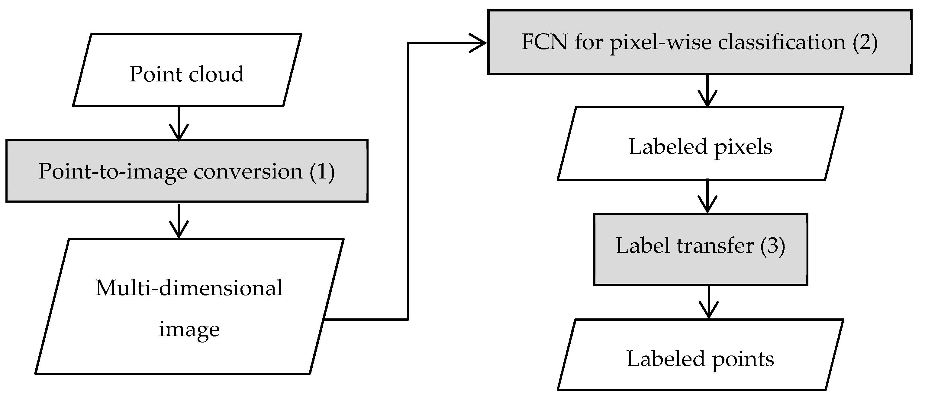
Figure 1.
The general workflow of the proposed classification approach.
Figure 1.
The general workflow of the proposed classification approach.
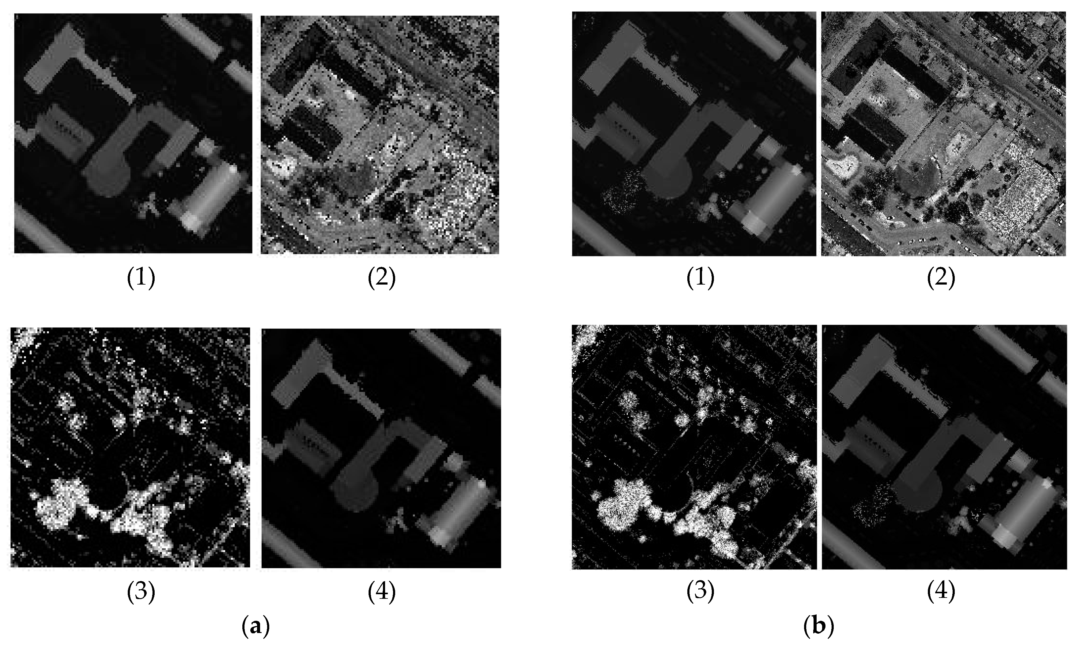
Figure 2.
Subset of extracted images from different pixel sizes: (a) 1 m; (b) 0.5 m. Each image has four feature channels: (1) elevation, (2) intensity, (3) return number, and (4) height difference between the lowest point in a 20 × 20 m neighborhood, and the lowest point in a pixel. A higher resolution image captures more detailed structures.
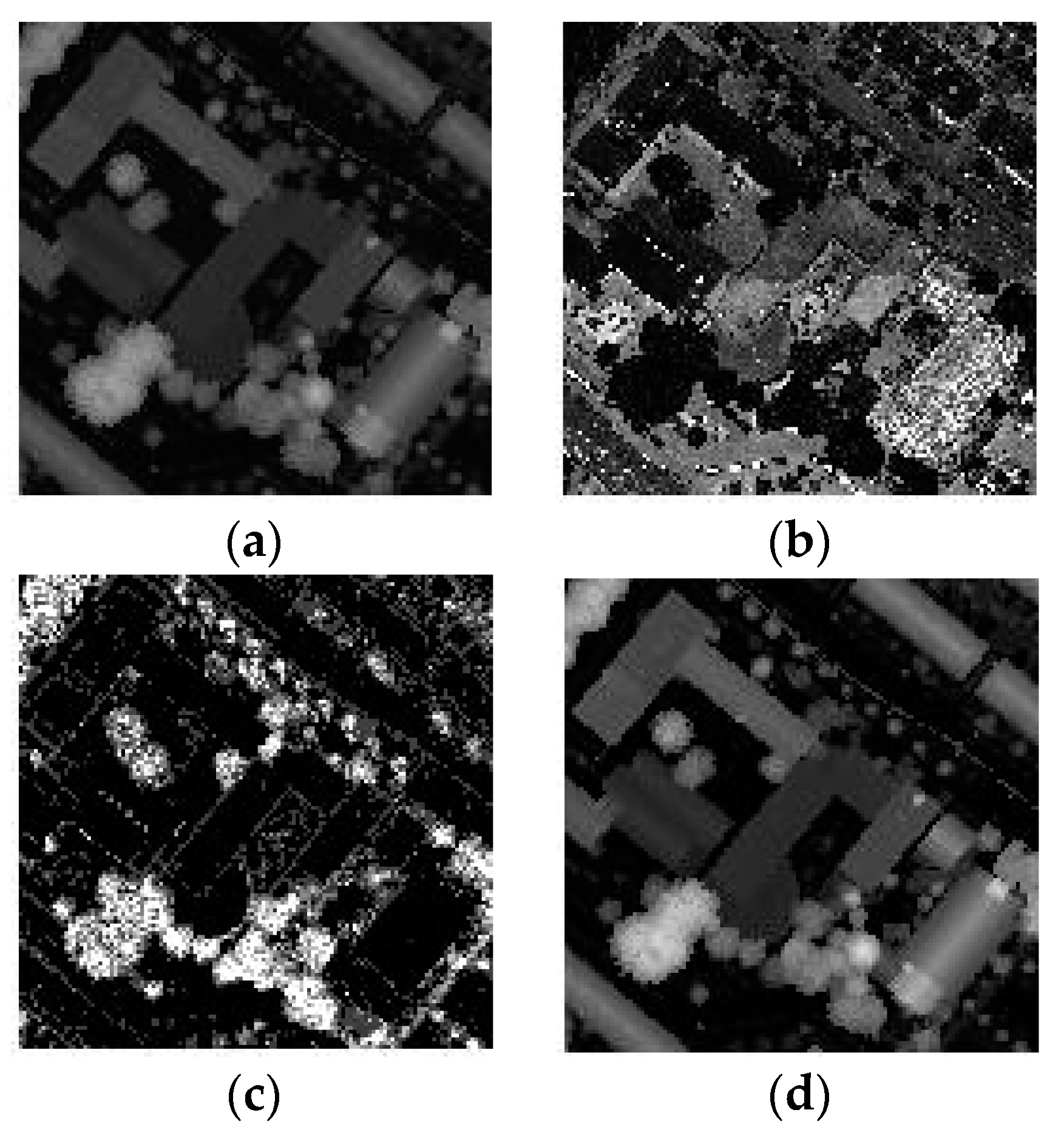
Figure 3.
Images from the highest point within each pixel: (a) elevation; (b) intensity; (c) the number of returns; (d) height difference between the highest point in a pixel and the lowest point in a 20 × 20 m neighborhood.
Figure 3.
Images from the highest point within each pixel: (a) elevation; (b) intensity; (c) the number of returns; (d) height difference between the highest point in a pixel and the lowest point in a 20 × 20 m neighborhood.
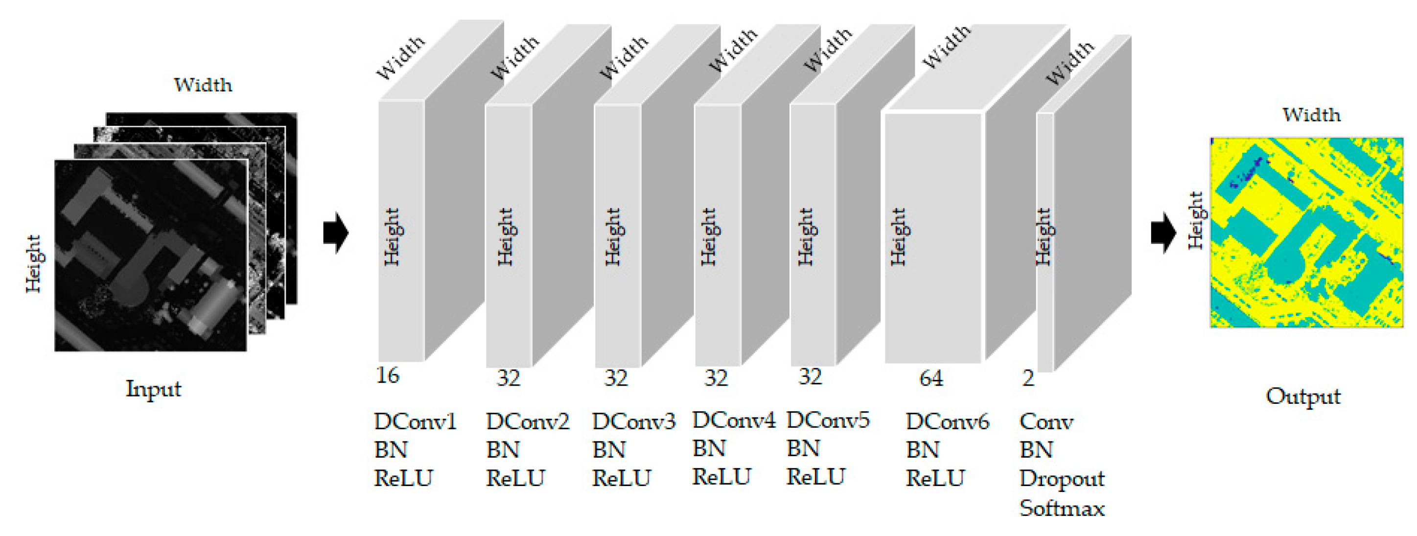
Figure 4.
The Fully Convolutional Network with dilated kernel (FCN-DK) network architecture.
Figure 4.
The Fully Convolutional Network with dilated kernel (FCN-DK) network architecture.
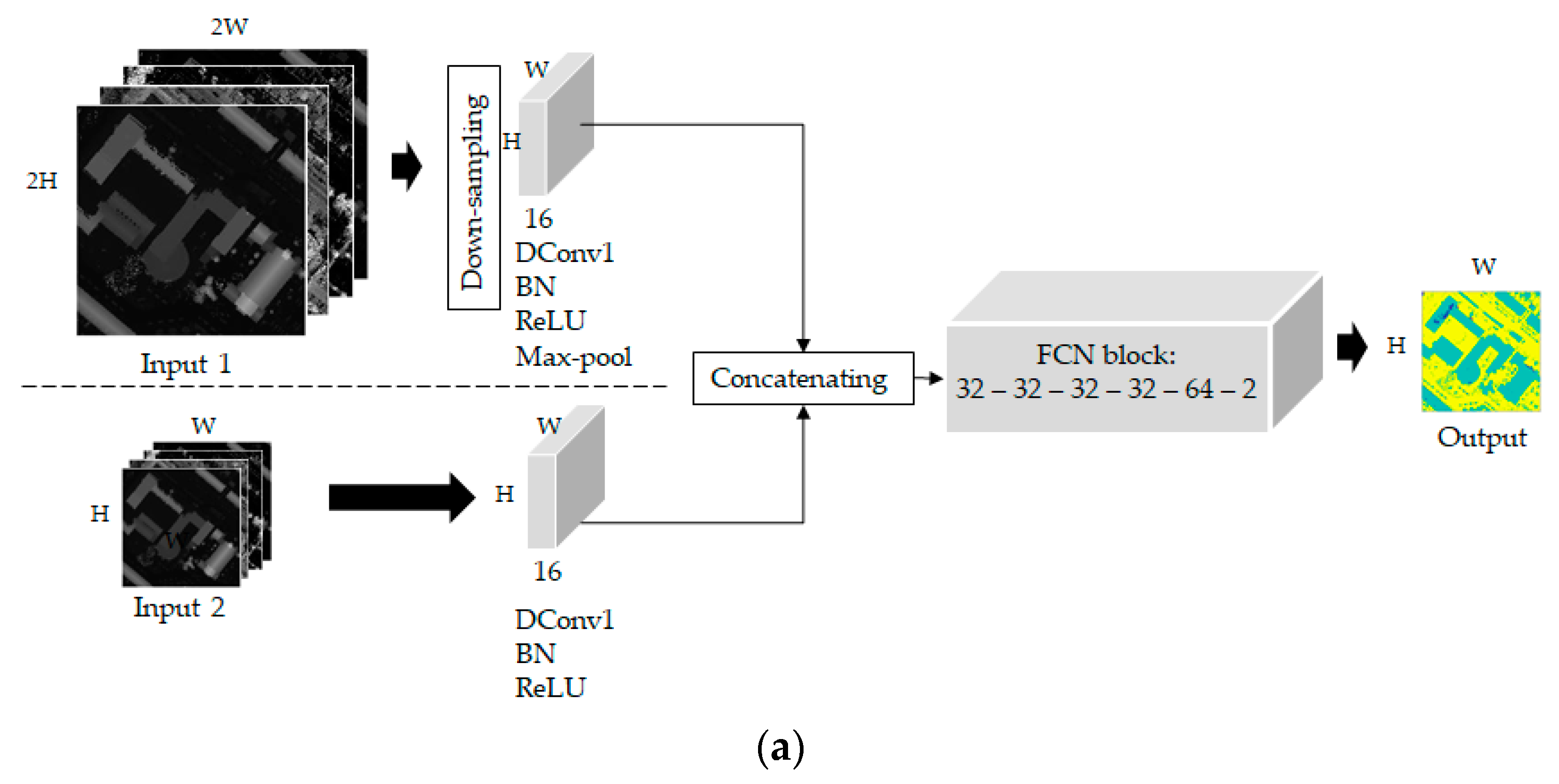
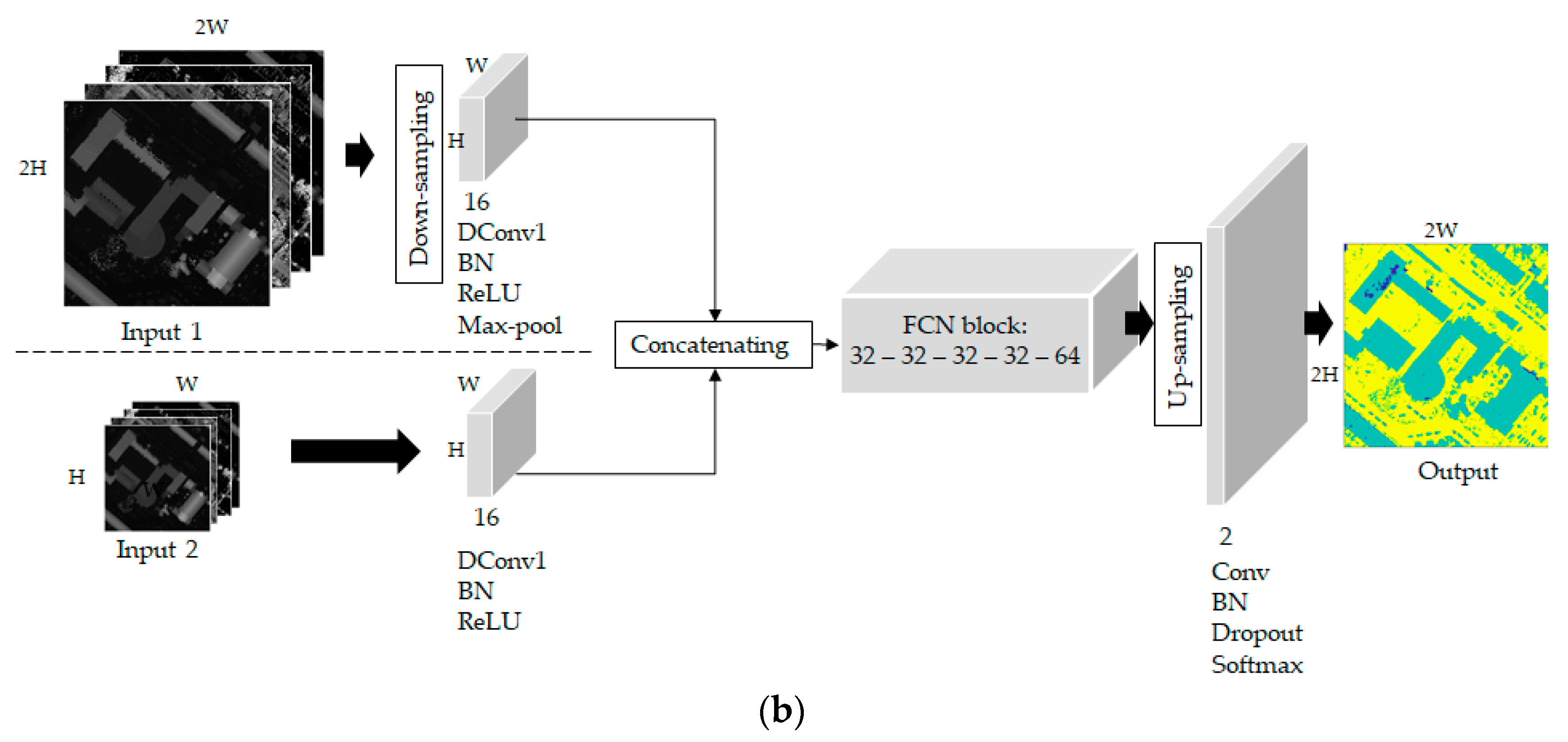
Figure 5.
The proposed multi-scale networks: (a) Multi-Scale (MS)-FCN Down (without up-sampling layer); (b) MS-FCN Down–Up (with up-sampling layer).
Figure 5.
The proposed multi-scale networks: (a) Multi-Scale (MS)-FCN Down (without up-sampling layer); (b) MS-FCN Down–Up (with up-sampling layer).
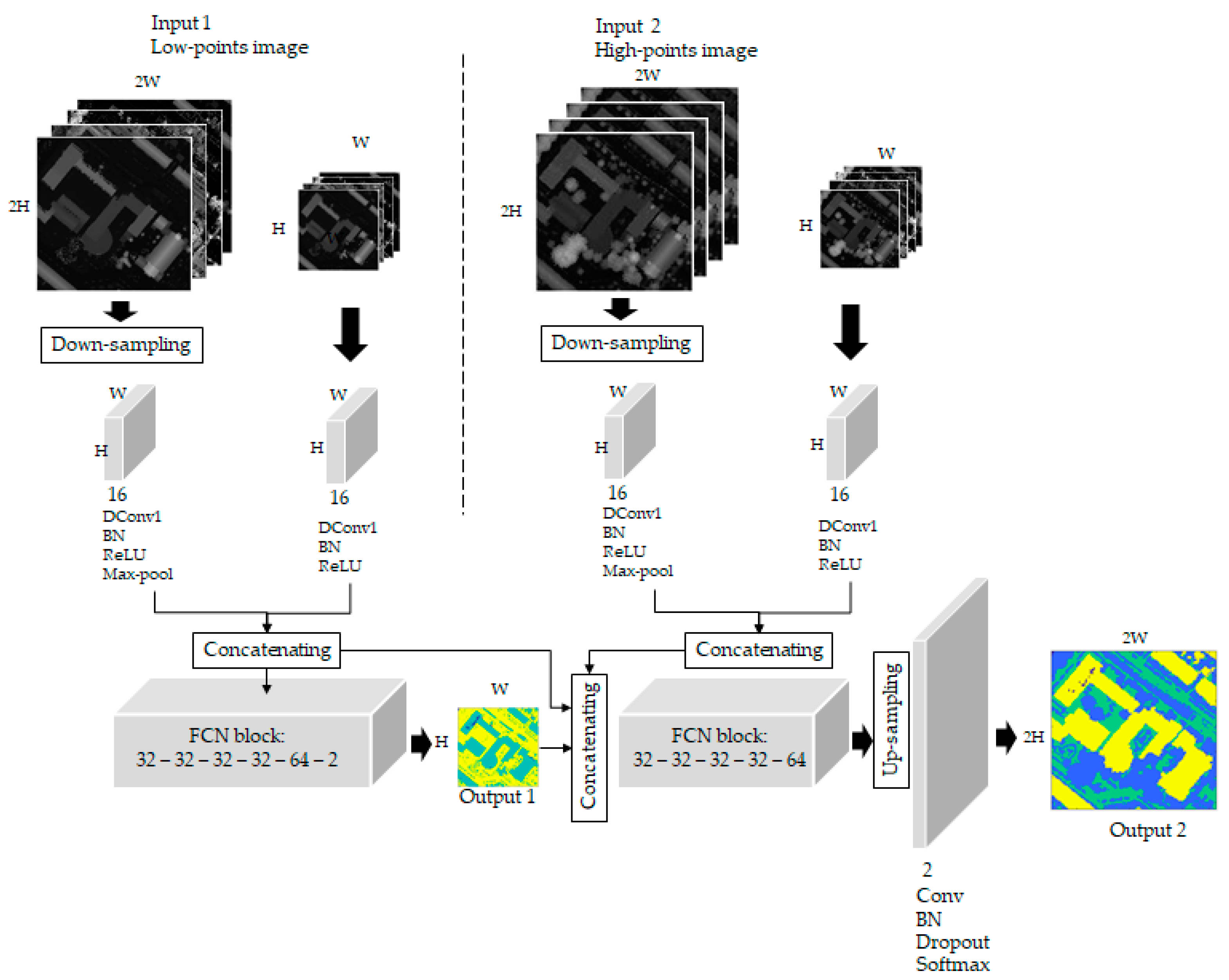
Figure 6.
The proposed Multi-Task Network (MTN)-FCN network for multi-class classification on a point cloud dataset.
Figure 6.
The proposed Multi-Task Network (MTN)-FCN network for multi-class classification on a point cloud dataset.
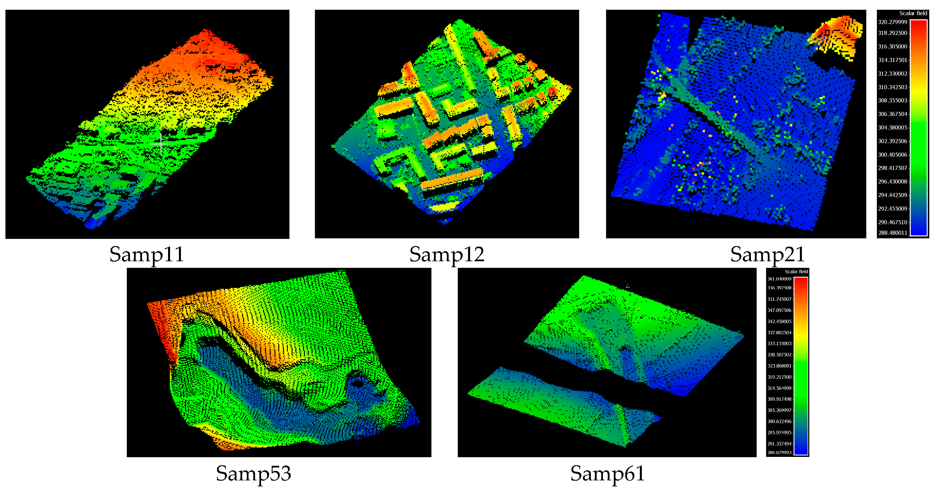
Figure 7.
Five sample areas of the International Society for Photogrammetry and Remote Sensing (ISPRS) dataset chosen for the testing set.
Figure 7.
Five sample areas of the International Society for Photogrammetry and Remote Sensing (ISPRS) dataset chosen for the testing set.
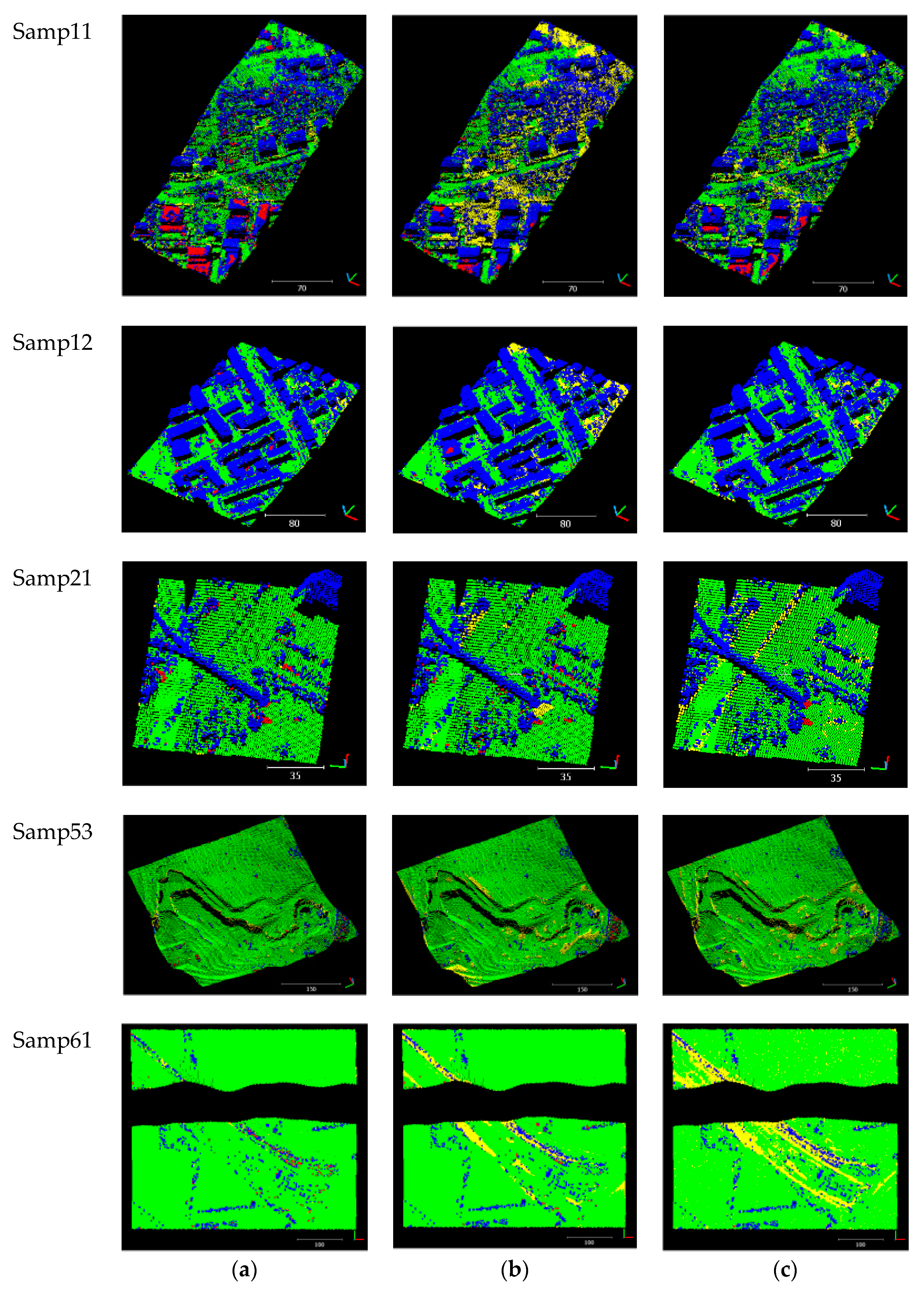
Figure 8.
Results on five testing samples of the ISPRS dataset: (a) FCN-DK; (b) Convolutional Neural Network (CNN); (c) LAStools software. Green: correctly labeled ground; Blue: correctly labeled non-ground; Yellow: ground point misclassified as non-ground; Red: non-ground point misclassified as ground.
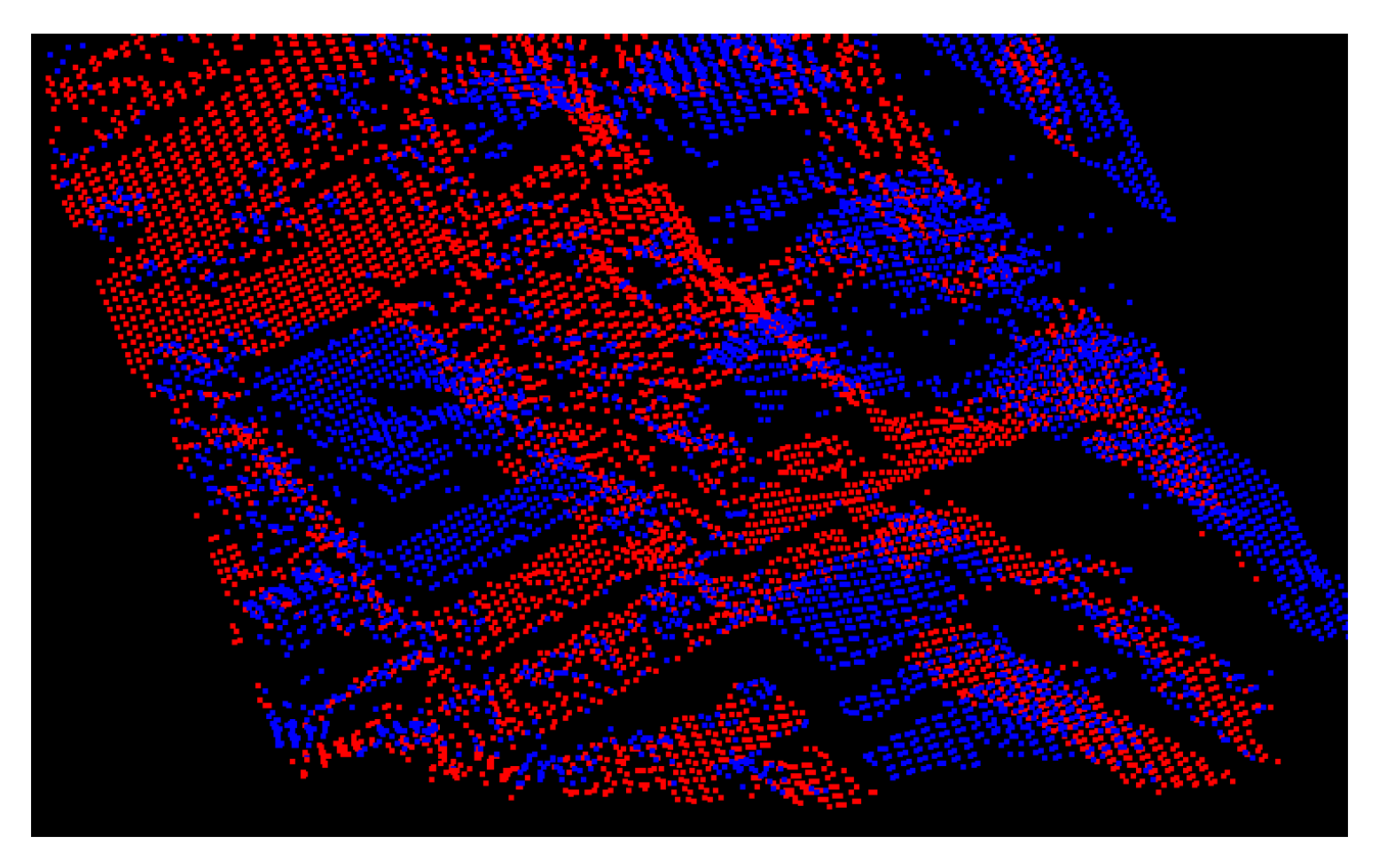
Figure 9.
A step-wise pattern on the houses in Samp11. Red: ground; blue: non-ground.
Figure 9.
A step-wise pattern on the houses in Samp11. Red: ground; blue: non-ground.
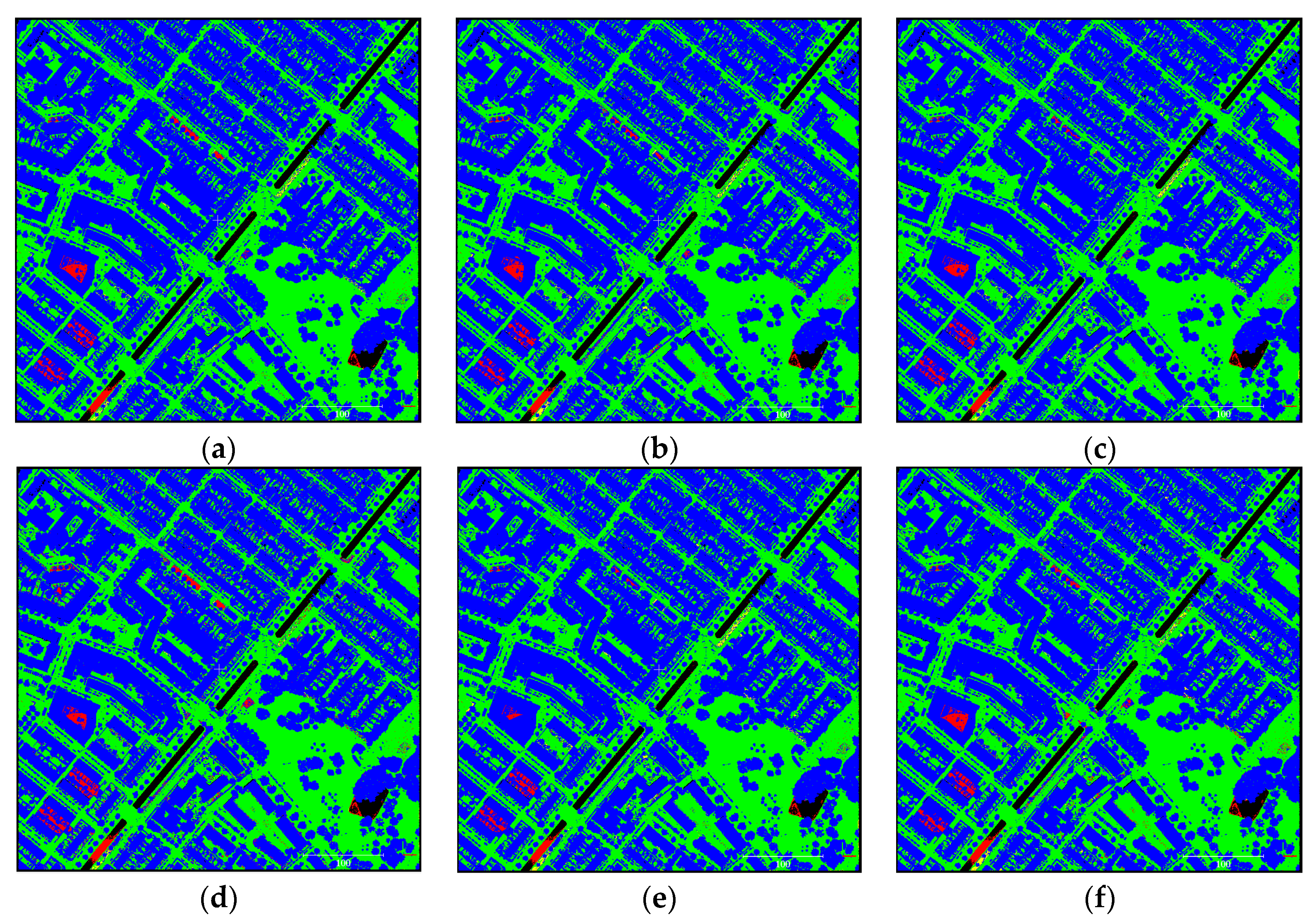
Figure 10.
Ground classification results on testing sample number 7 (TS7) of the Actueel Hoogtebestand Nederland 3 (AHN3) dataset: (a) FCN 1 m; (b) FCN 0.5 m; (c) MS-FCN Down; (d) MS-FCN Down–Up; (e) MTN-FCN; (f) LAStools. Green: correctly labeled ground; Blue: correctly labeled non-ground; Yellow: ground point misclassified as non-ground; Red: non-ground point misclassified as ground.
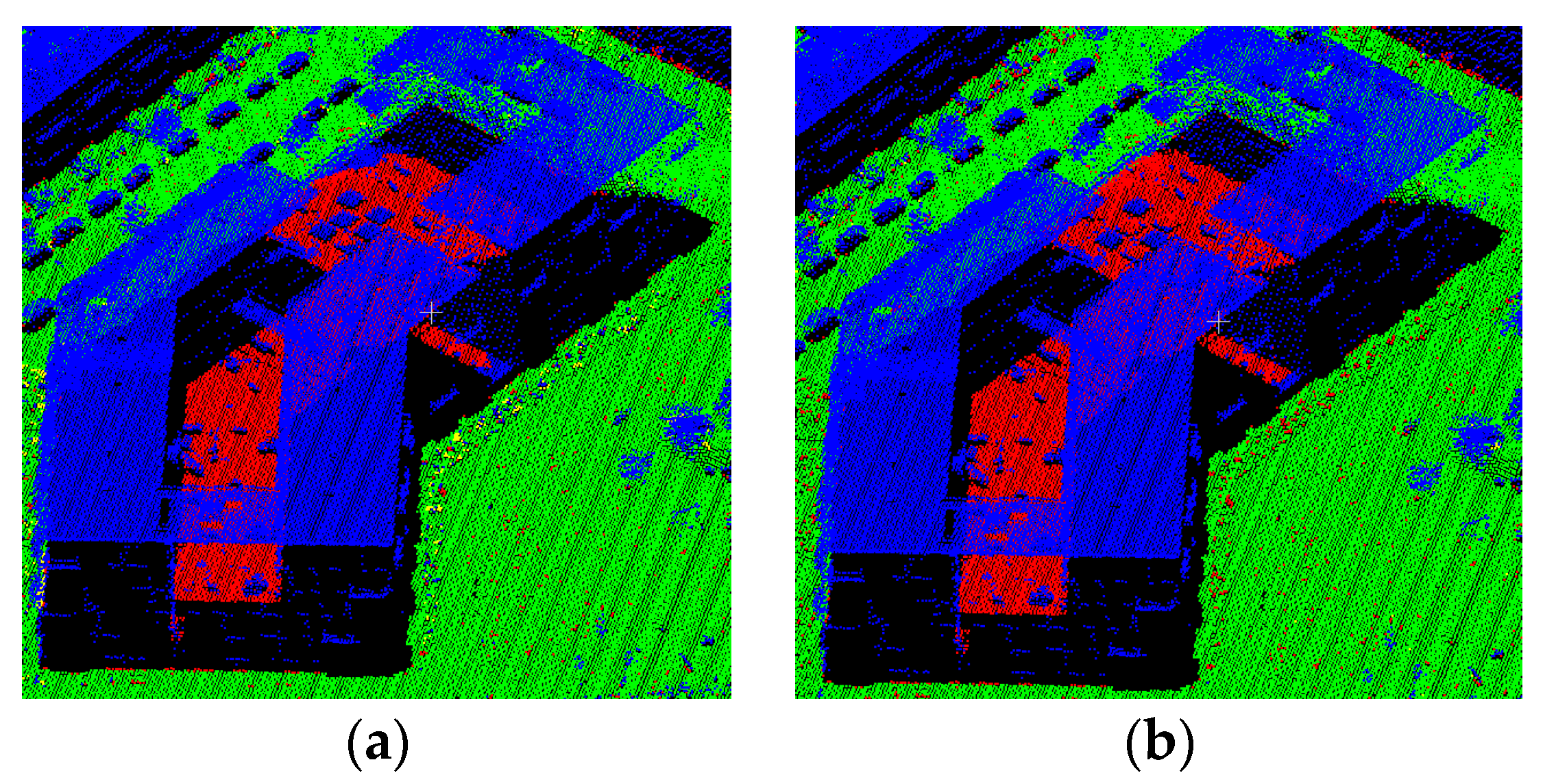
Figure 11.
Error result on a very large building: (a) FCN; (b) LAStools. Red points are those incorrectly labeled as ground points.
Figure 11.
Error result on a very large building: (a) FCN; (b) LAStools. Red points are those incorrectly labeled as ground points.
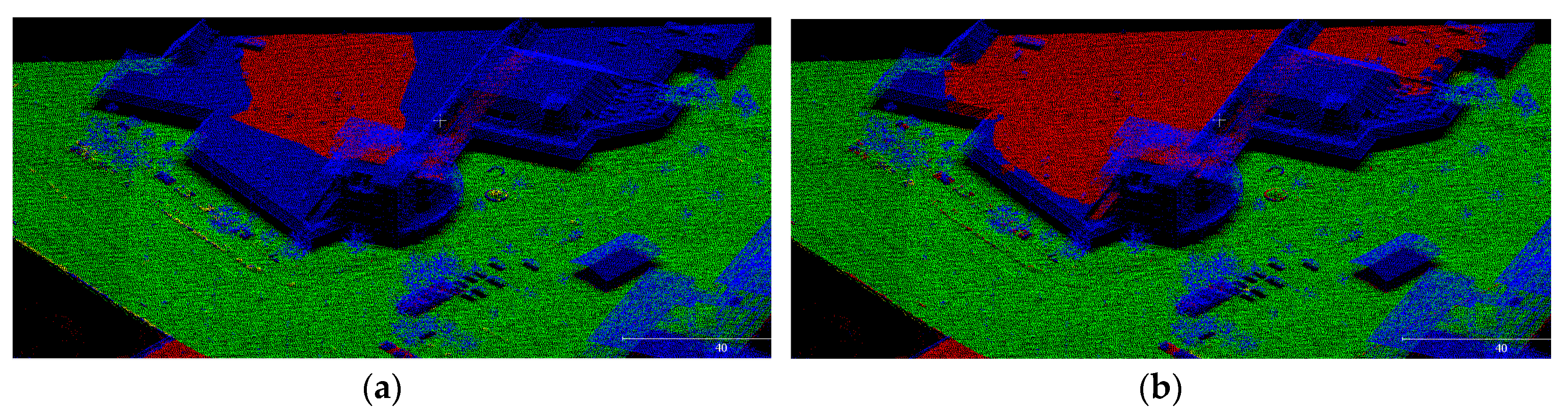
Figure 12.
Error result on a large building with a lower roof in the middle: (a) FCN; (b) LAStools. Red points are those incorrectly labeled as ground points.
Figure 12.
Error result on a large building with a lower roof in the middle: (a) FCN; (b) LAStools. Red points are those incorrectly labeled as ground points.
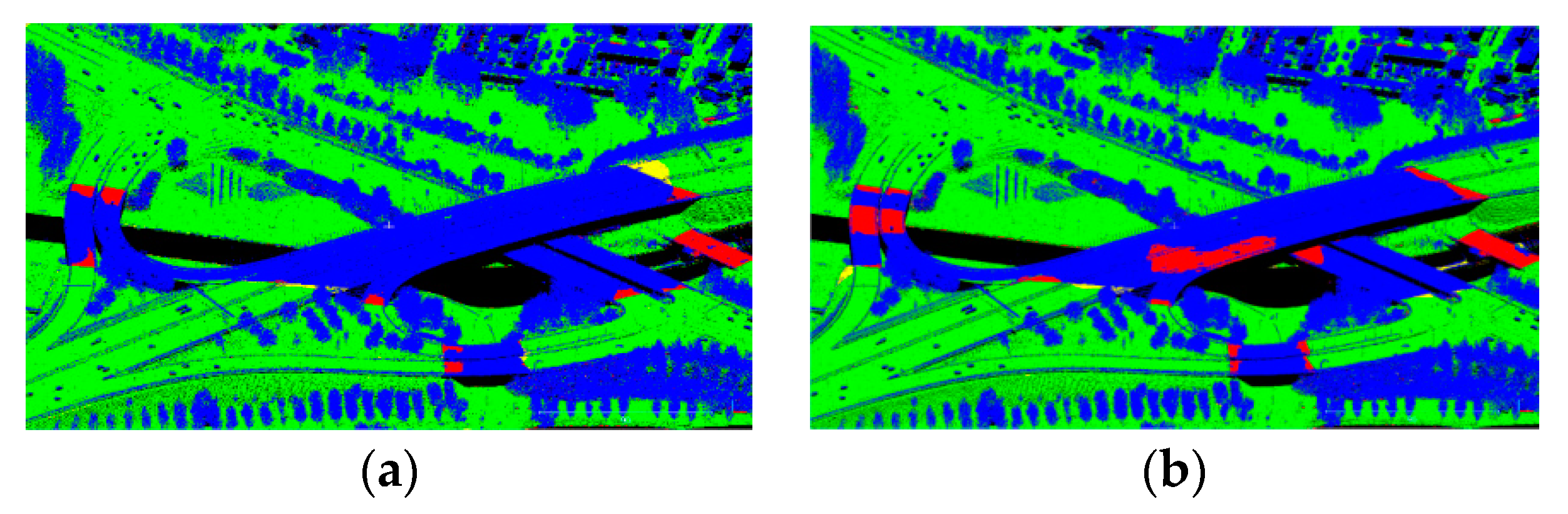
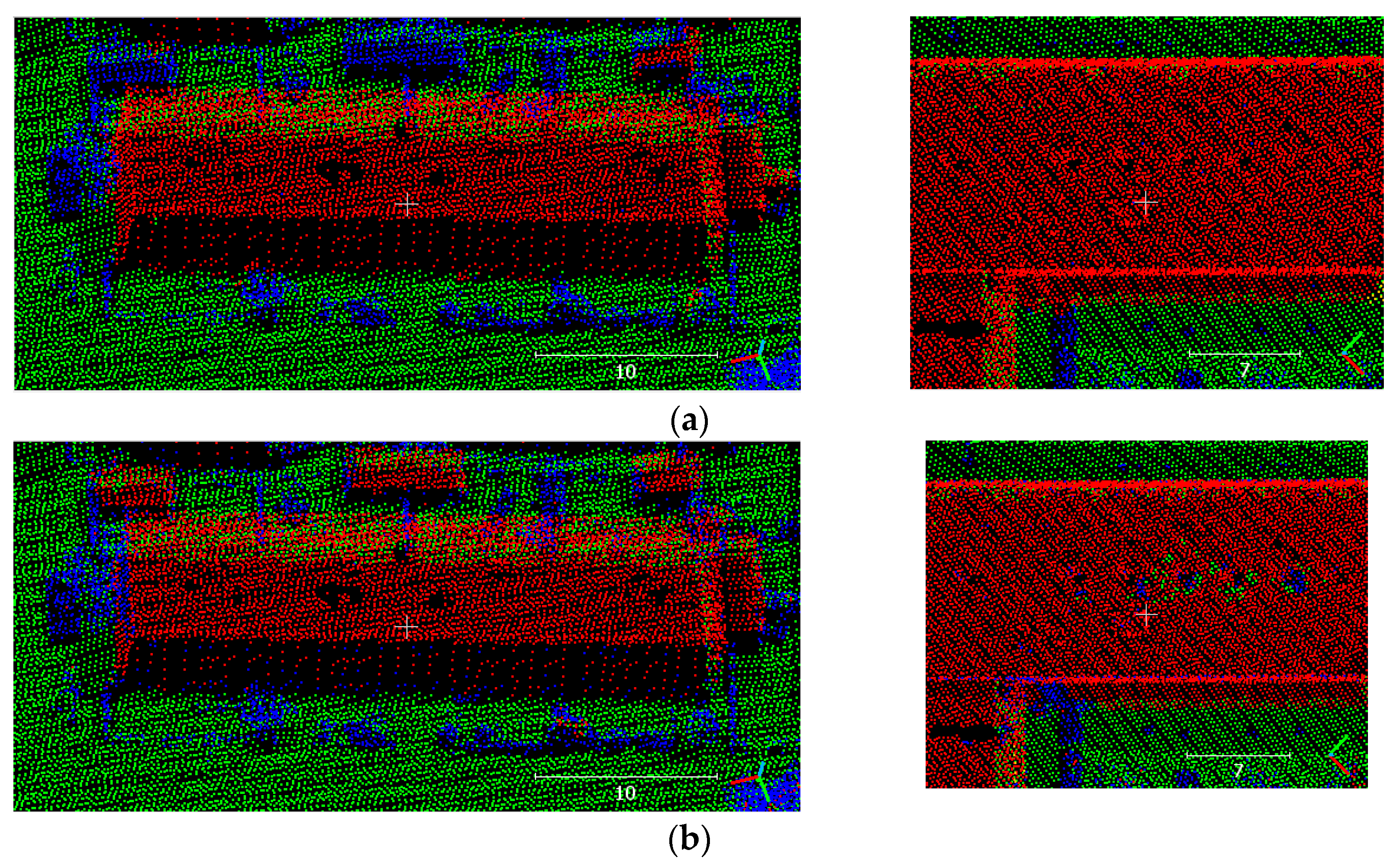
Figure 13.
Errors on flat bridges. Red points are those incorrectly labeled as ground points.
Figure 13.
Errors on flat bridges. Red points are those incorrectly labeled as ground points.
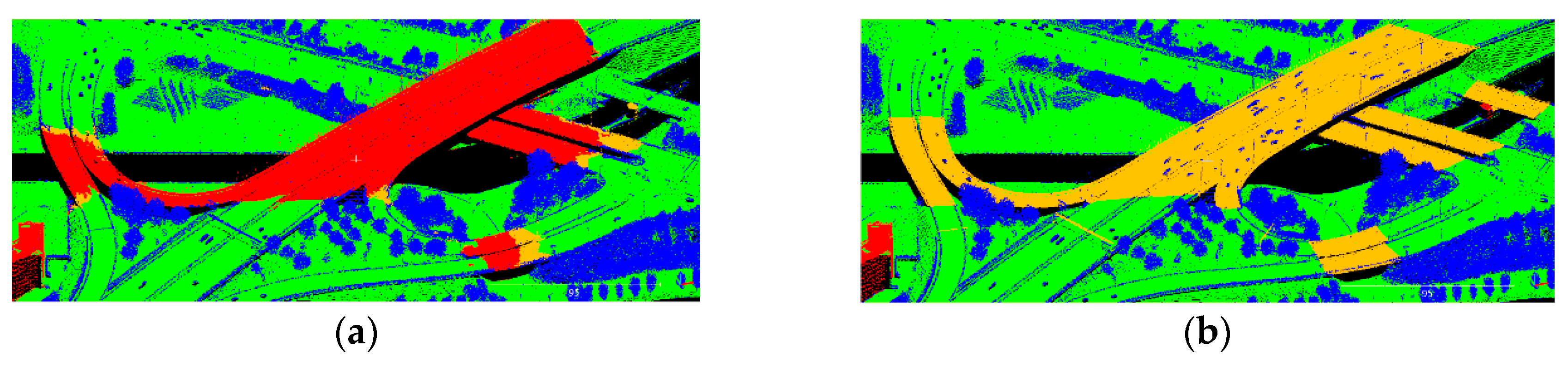
Figure 14.
Result on a mixed structure of road and bridge: (a) FCN; (b) LAStools. Red points are those incorrectly labeled as ground points. Yellow points are those incorecctly labeled as non-ground points.
Figure 14.
Result on a mixed structure of road and bridge: (a) FCN; (b) LAStools. Red points are those incorrectly labeled as ground points. Yellow points are those incorecctly labeled as non-ground points.
Figure 15.
A situation when LAStools failed to detect a relatively flat ground surface: (a) FCN; (b) LAStools.
Figure 15.
A situation when LAStools failed to detect a relatively flat ground surface: (a) FCN; (b) LAStools.
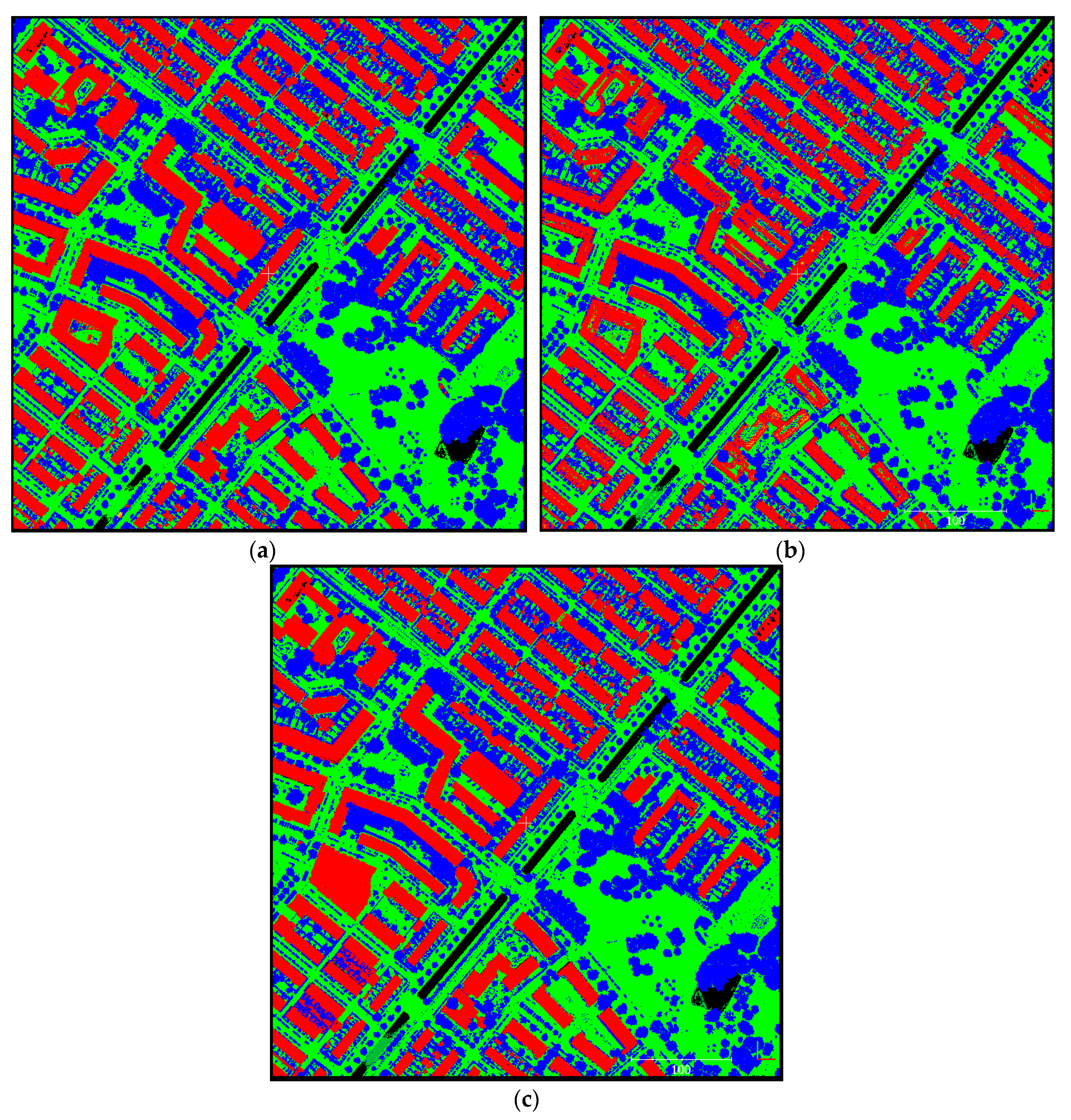
Figure 16.
Multi-class classification results on sample TS7 of the AHN3 dataset: (a) MTN-FCN; (b) Random Forest (RF); (c) Reference. Green: ground; blue: vegetation; red: building; dark green: water.
Figure 16.
Multi-class classification results on sample TS7 of the AHN3 dataset: (a) MTN-FCN; (b) Random Forest (RF); (c) Reference. Green: ground; blue: vegetation; red: building; dark green: water.
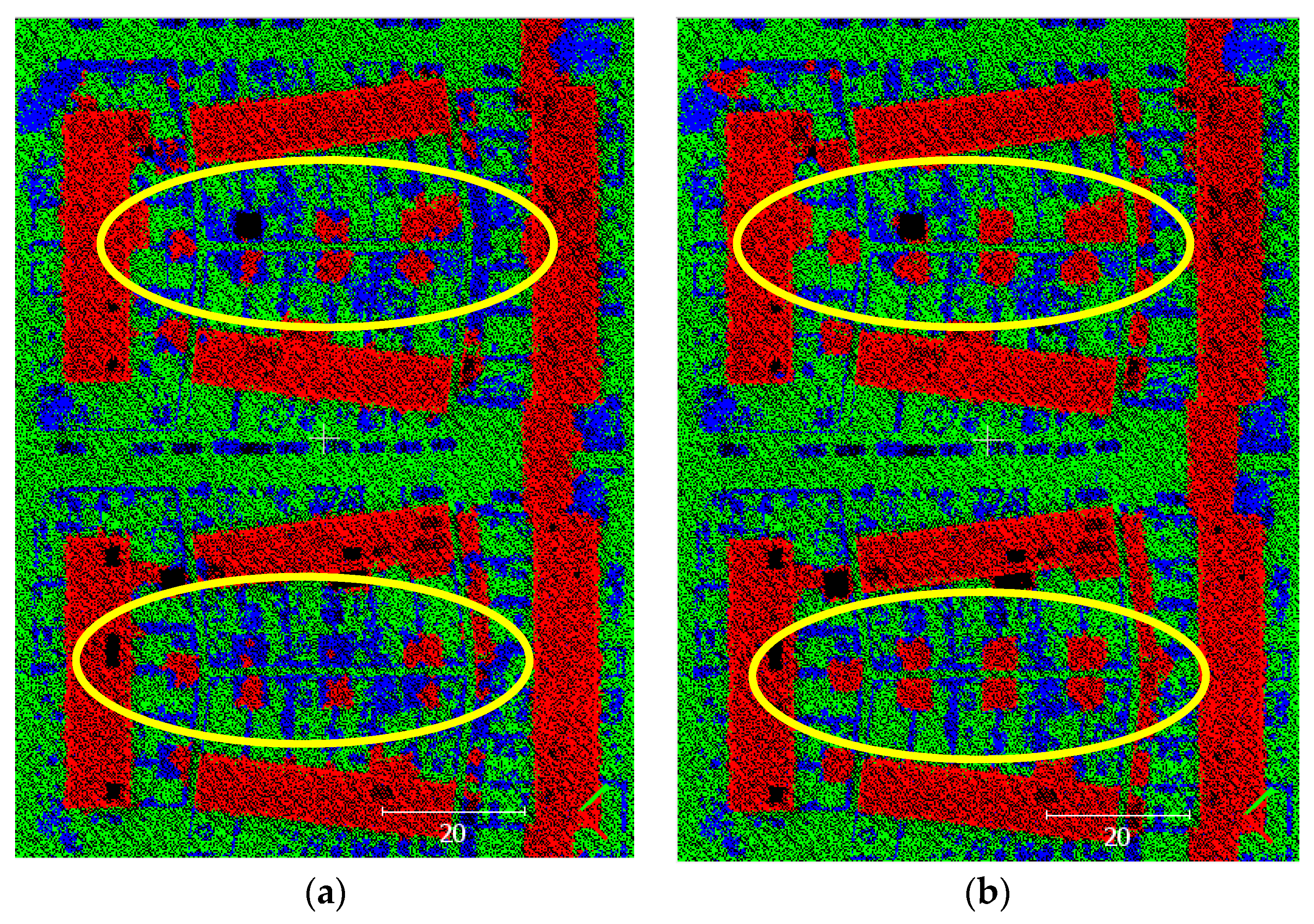
Figure 17.
Difference between: (a) single pixel (1-m) MTN-FCN; (b): multi-scale MTN-FCN. Note the shape of the small building roofs.
Figure 17.
Difference between: (a) single pixel (1-m) MTN-FCN; (b): multi-scale MTN-FCN. Note the shape of the small building roofs.
Figure 18.
Error on FCN result due to noise in sample TS5: (a) prediction; (b) reference; (c) noise in one building in TS5; (d) noise in one building in the training set. Note that noise in (c) is higher than in (d).
Figure 18.
Error on FCN result due to noise in sample TS5: (a) prediction; (b) reference; (c) noise in one building in TS5; (d) noise in one building in the training set. Note that noise in (c) is higher than in (d).
Figure 19.
Elevated bridge: (a) FCN; (b) reference. Green: ground; blue: vegetation; red: building; yellow: bridge.
Figure 19.
Elevated bridge: (a) FCN; (b) reference. Green: ground; blue: vegetation; red: building; yellow: bridge.
Figure 20.
Comparison results: (a) FCN; (b) RF.
Figure 20.
Comparison results: (a) FCN; (b) RF.
Table 1.
The detailed architecture of the network.
Table 1.
The detailed architecture of the network.
| Layer | Filter Size | Number of Filters | Dilation Factor | Receptive Field Size (Pixel) | Memory Required (Megabytes) |
|---|
| DConv1 | 5 × 5 | 16 | 1 | 5 × 5 | 22 |
| DConv2 | 5 × 5 | 32 | 2 | 13 × 13 | 43 |
| DConv3 | 5 × 5 | 32 | 3 | 25 × 25 | 43 |
| DConv4 | 5 × 5 | 32 | 4 | 41 × 41 | 43 |
| DConv5 | 5 × 5 | 32 | 5 | 61 × 61 | 43 |
| DConv6 | 5 × 5 | 64 | 6 | 85 × 85 | 86 |
| Conv | 1 × 1 | 2 | - | 1 × 1 | 3 |
Table 2.
Total error on ISPRS dataset.
Table 2.
Total error on ISPRS dataset.
| Sample | FCN-DK6 | CNN [11] | LAStools |
|---|
| Samp11 | 15.01 | 19.47 | 17.67 |
| Samp12 | 3.44 | 7.99 | 6.97 |
| Samp21 | 1.6 | 2.23 | 6.66 |
| Samp53 | 4.75 | 5.67 | 14.37 |
| Samp61 | 1.27 | 4.20 | 17.24 |
| Average | 5.21 | 7.91 | 12.58 |
Table 3.
Type-I error on ISPRS dataset.
Table 3.
Type-I error on ISPRS dataset.
| Sample | FCN-DK6 | CNN | LAStools |
|---|
| Samp11 | 14.09 | 27.10 | 26.94 |
| Samp12 | 2.52 | 13.92 | 12.87 |
| Samp21 | 0.24 | 1.63 | 7.98 |
| Samp53 | 3.92 | 4.44 | 14.84 |
| Samp61 | 0.61 | 3.95 | 17.85 |
| Average | 4.28 | 10.21 | 16.10 |
Table 4.
Type-II error on ISPRS dataset.
Table 4.
Type-II error on ISPRS dataset.
| Sample | FCN-DK6 | CNN | LAStools |
|---|
| Samp11 | 16.25 | 9.20 | 5.18 |
| Samp12 | 4.41 | 1.75 | 0.77 |
| Samp21 | 6.53 | 4.39 | 1.87 |
| Samp53 | 24.49 | 34.79 | 3.24 |
| Samp61 | 19.72 | 11.06 | 0.40 |
| Average | 14.28 | 12.24 | 2.29 |
Table 5.
Total errors of the AHN3 dataset.
Table 5.
Total errors of the AHN3 dataset.
| Sample | FCN 1 m | FCN 0.5 m | MS-FCN Down | MS-FCN Down–Up | MTN-FCN | LAStools |
|---|
| TS 1 | 4.21 | 5.77 | 4.00 | 4.80 | 3.78 | 5.08 |
| TS 2 | 2.48 | 3.07 | 3.02 | 3.78 | 2.60 | 3.44 |
| TS 3 | 1.94 | 1.94 | 1.96 | 2.93 | 1.87 | 2.32 |
| TS 4 | 2.52 | 2.08 | 1.96 | 3.06 | 1.96 | 2.46 |
| TS 5 | 2.47 | 5.06 | 3.69 | 3.55 | 4.15 | 6.23 |
| TS 6 | 2.59 | 2.24 | 2.47 | 3.13 | 2.44 | 4.08 |
| TS 7 | 1.82 | 1.79 | 1.71 | 2.81 | 1.71 | 2.05 |
| TS 8 | 2.24 | 2.35 | 2.40 | 3.25 | 2.20 | 2.86 |
| TS 9 | 4.48 | 3.13 | 2.75 | 2.93 | 2.71 | 3.38 |
| TS 10 | 3.12 | 3.79 | 2.91 | 3.91 | 2.97 | 3.23 |
| Average | 2.79 | 3.12 | 2.69 | 3.42 | 2.64 | 3.51 |
Table 6.
Type-I errors of the AHN3 dataset.
Table 6.
Type-I errors of the AHN3 dataset.
| Sample | FCN 1 m | FCN 0.5 m | MS-FCN Down | MS-FCN Down–Up | MTN-FCN | LAStools |
|---|
| TS 1 | 2.09 | 3.77 | 2.63 | 0.71 | 2.17 | 1.70 |
| TS 2 | 1.49 | 1.73 | 2.72 | 1.69 | 1.65 | 1.98 |
| TS 3 | 0.89 | 0.38 | 0.88 | 0.98 | 0.86 | 1.27 |
| TS 4 | 2.48 | 0.58 | 1.42 | 1.07 | 1.38 | 1.03 |
| TS 5 | 2.15 | 6.02 | 4.50 | 2.70 | 5.34 | 6.04 |
| TS 6 | 1.26 | 0.36 | 1.27 | 0.53 | 1.23 | 2.61 |
| TS 7 | 1.01 | 0.51 | 1.03 | 1.00 | 1.03 | 1.72 |
| TS 8 | 1.42 | 0.86 | 1.28 | 0.99 | 1.35 | 2.01 |
| TS 9 | 5.40 | 2.55 | 1.68 | 0.90 | 1.68 | 1.41 |
| TS 10 | 3.11 | 1.98 | 1.84 | 1.47 | 2.13 | 1.55 |
| Average | 2.13 | 1.87 | 1.93 | 1.20 | 1.88 | 2.13 |
Table 7.
Type-II errors of the AHN3 dataset.
Table 7.
Type-II errors of the AHN3 dataset.
| Sample | FCN 1 m | FCN 0.5 m | MS-FCN Down | MS-FCN Down–Up | MTN-FCN | LAStools |
|---|
| TS 1 | 6.61 | 8.03 | 5.55 | 9.44 | 5.61 | 8.91 |
| TS 2 | 3.51 | 4.46 | 3.32 | 5.94 | 3.57 | 4.94 |
| TS 3 | 2.83 | 3.28 | 2.89 | 4.59 | 2.74 | 3.21 |
| TS 4 | 2.54 | 3.24 | 2.38 | 4.59 | 2.40 | 3.56 |
| TS 5 | 2.96 | 3.60 | 2.46 | 4.82 | 2.36 | 6.54 |
| TS 6 | 4.06 | 4.34 | 3.81 | 6.02 | 3.79 | 5.71 |
| TS 7 | 2.44 | 2.78 | 2.23 | 4.20 | 2.23 | 2.31 |
| TS 8 | 2.81 | 3.38 | 3.18 | 4.83 | 2.79 | 3.46 |
| TS 9 | 3.56 | 3.71 | 3.83 | 4.97 | 3.75 | 5.36 |
| TS 10 | 3.12 | 6.20 | 4.35 | 7.19 | 4.09 | 5.47 |
| Average | 3.44 | 4.30 | 3.40 | 5.66 | 3.33 | 4.95 |
Table 8.
Precision values of the AHN3 dataset. TS: testing set.
Table 8.
Precision values of the AHN3 dataset. TS: testing set.
| Class | Method | TS 1 | TS 2 | TS 3 | TS 4 | TS 5 | TS 6 | TS 7 | TS 8 | TS 9 | TS 10 | Average |
|---|
| Vegetation | MTN-FCN | 0.93 | 0.91 | 0.96 | 0.96 | 0.74 | 0.89 | 0.96 | 0.97 | 0.96 | 0.95 | 0.92 |
| RF | 0.87 | 0.93 | 0.92 | 0.94 | 0.87 | 0.89 | 0.92 | 0.97 | 0.96 | 0.94 | 0.92 |
| Ground | MTN-FCN | 0.95 | 0.97 | 0.97 | 0.97 | 0.98 | 0.97 | 0.97 | 0.96 | 0.96 | 0.97 | 0.97 |
| RF | 0.95 | 0.96 | 0.96 | 0.95 | 0.97 | 0.97 | 0.95 | 0.93 | 0.93 | 0.95 | 0.95 |
| Building | MTN-FCN | 0.95 | 0.96 | 0.96 | 0.95 | 0.97 | 0.98 | 0.96 | 0.94 | 0.94 | 0.48 | 0.91 |
| RF | 0.94 | 0.91 | 0.97 | 0.93 | 0.89 | 0.97 | 0.95 | 0.92 | 0.63 | 0.32 | 0.85 |
| Average Precision | MTN-FCN | 0.94 | 0.95 | 0.96 | 0.96 | 0.90 | 0.95 | 0.96 | 0.96 | 0.95 | 0.80 | 0.93 |
| RF | 0.92 | 0.93 | 0.95 | 0.94 | 0.91 | 0.94 | 0.95 | 0.94 | 0.84 | 0.74 | 0.91 |
Table 9.
Recall values of the AHN3 dataset. MTN: Multi-Task Network, RF: Random Forest.
Table 9.
Recall values of the AHN3 dataset. MTN: Multi-Task Network, RF: Random Forest.
| Class | Method | TS 1 | TS 2 | TS 3 | TS 4 | TS 5 | TS 6 | TS 7 | TS 8 | TS 9 | TS 10 | Average |
|---|
| Vegetation | MTN-FCN | 0.87 | 0.95 | 0.95 | 0.95 | 0.95 | 0.95 | 0.96 | 0.97 | 0.98 | 0.95 | 0.95 |
| RF | 0.97 | 0.91 | 0.95 | 0.94 | 0.89 | 0.93 | 0.95 | 0.95 | 0.95 | 0.92 | 0.94 |
| Ground | MTN-FCN | 0.98 | 0.98 | 0.99 | 0.97 | 0.95 | 0.99 | 0.99 | 0.99 | 0.98 | 0.98 | 0.98 |
| RF | 0.97 | 0.98 | 0.99 | 0.98 | 0.96 | 0.99 | 0.99 | 0.99 | 0.92 | 0.89 | 0.97 |
| Building | MTN-FCN | 0.96 | 0.86 | 0.94 | 0.95 | 0.77 | 0.87 | 0.94 | 0.86 | 0.93 | 0.92 | 0.90 |
| RF | 0.89 | 0.88 | 0.87 | 0.88 | 0.87 | 0.89 | 0.84 | 0.80 | 0.78 | 0.87 | 0.86 |
| Average Recall | MTN-FCN | 0.94 | 0.93 | 0.96 | 0.96 | 0.89 | 0.94 | 0.96 | 0.94 | 0.96 | 0.95 | 0.94 |
| RF | 0.94 | 0.92 | 0.94 | 0.93 | 0.91 | 0.94 | 0.93 | 0.91 | 0.88 | 0.89 | 0.92 |
Table 10.
Computational time comparison. Computer specifications: Intel Core i7-6700HQ 2.6GHz, 16 GB RAM, and Nvidia Quadro M1000M 2GB.
Table 10.
Computational time comparison. Computer specifications: Intel Core i7-6700HQ 2.6GHz, 16 GB RAM, and Nvidia Quadro M1000M 2GB.
| Method | Point-to-Image Conversion | Training | Testing |
|---|
| FCN | 36 min | 12 h | 7.8 s |
| CNN | 47 h | 2.5 h | 126 s |


 ,
, 


