Learning a Multi-Branch Neural Network from Multiple Sources for Knowledge Adaptation in Remote Sensing Imagery

 ,
,  ,
, 

 and
and 
Abstract
1. Introduction
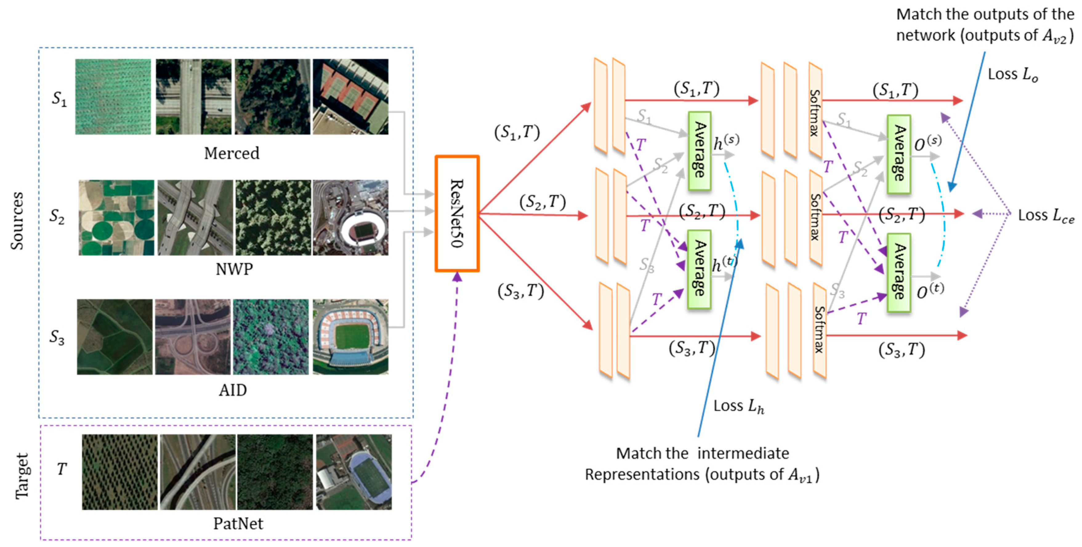
2. Description of the Proposed Method
2.1. Preliminaries
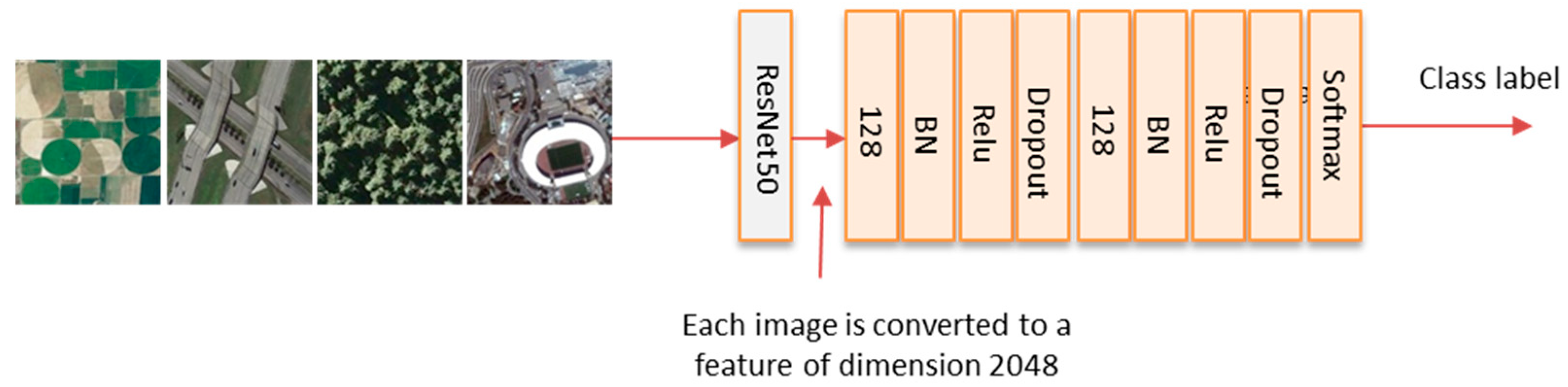
2.2. Model Architecture
2.3. Objective Function and Model Optimization
| MB-Net method. |
| Input: Source domains and one target domain |
| Output: Target class labels |
1: Set MB-Net parameters:
|
| 2: Pre-train the network on the M-labeled source domains using the Adam method (i.e., estimate the parameters by optimizing only the cross-entropy loss in Equation (2)) |
| 3: Set the number of mini-batches: |
4: For
|
| 5: Classify the target domain T. |
3. Experimental Results
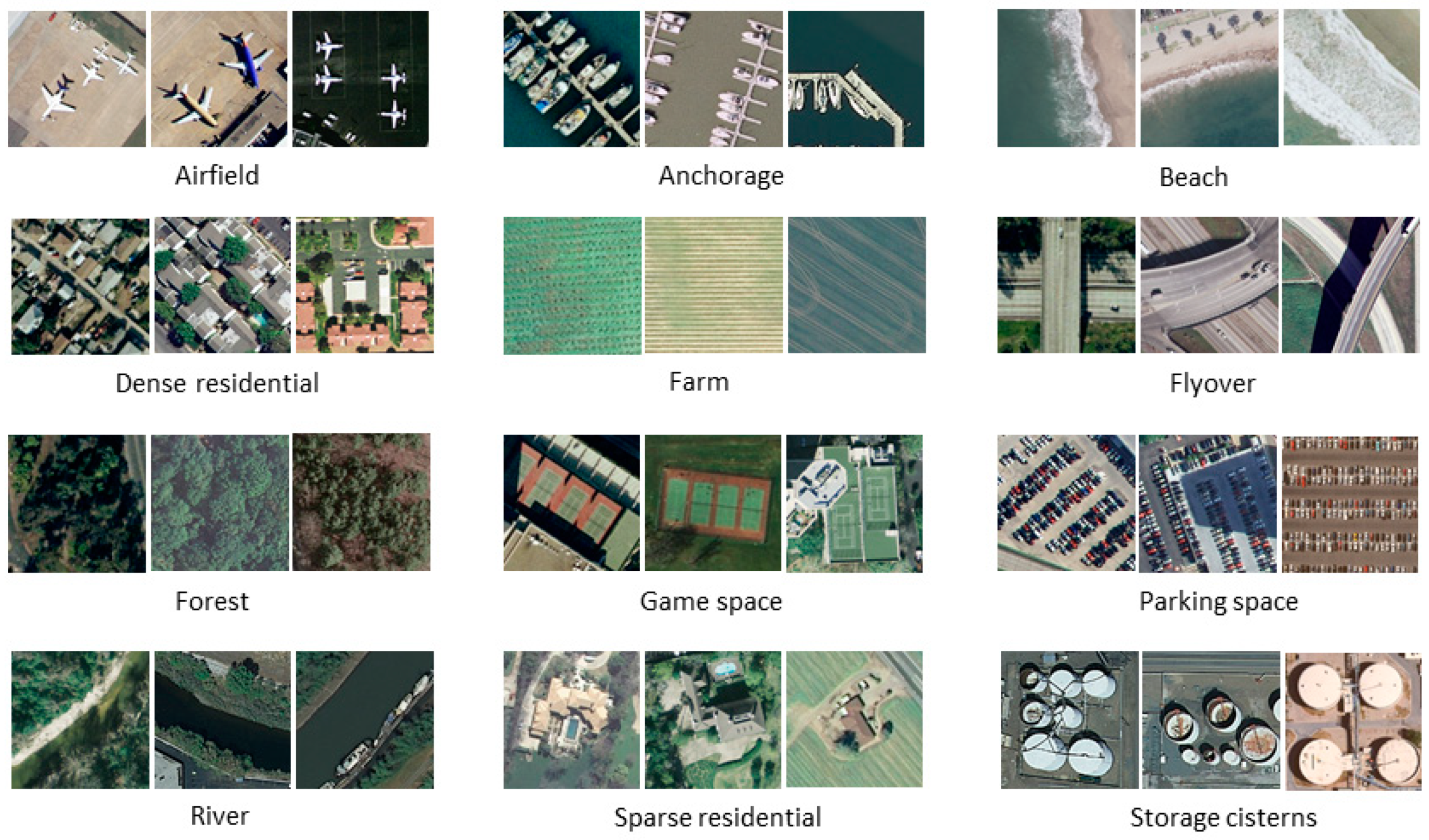
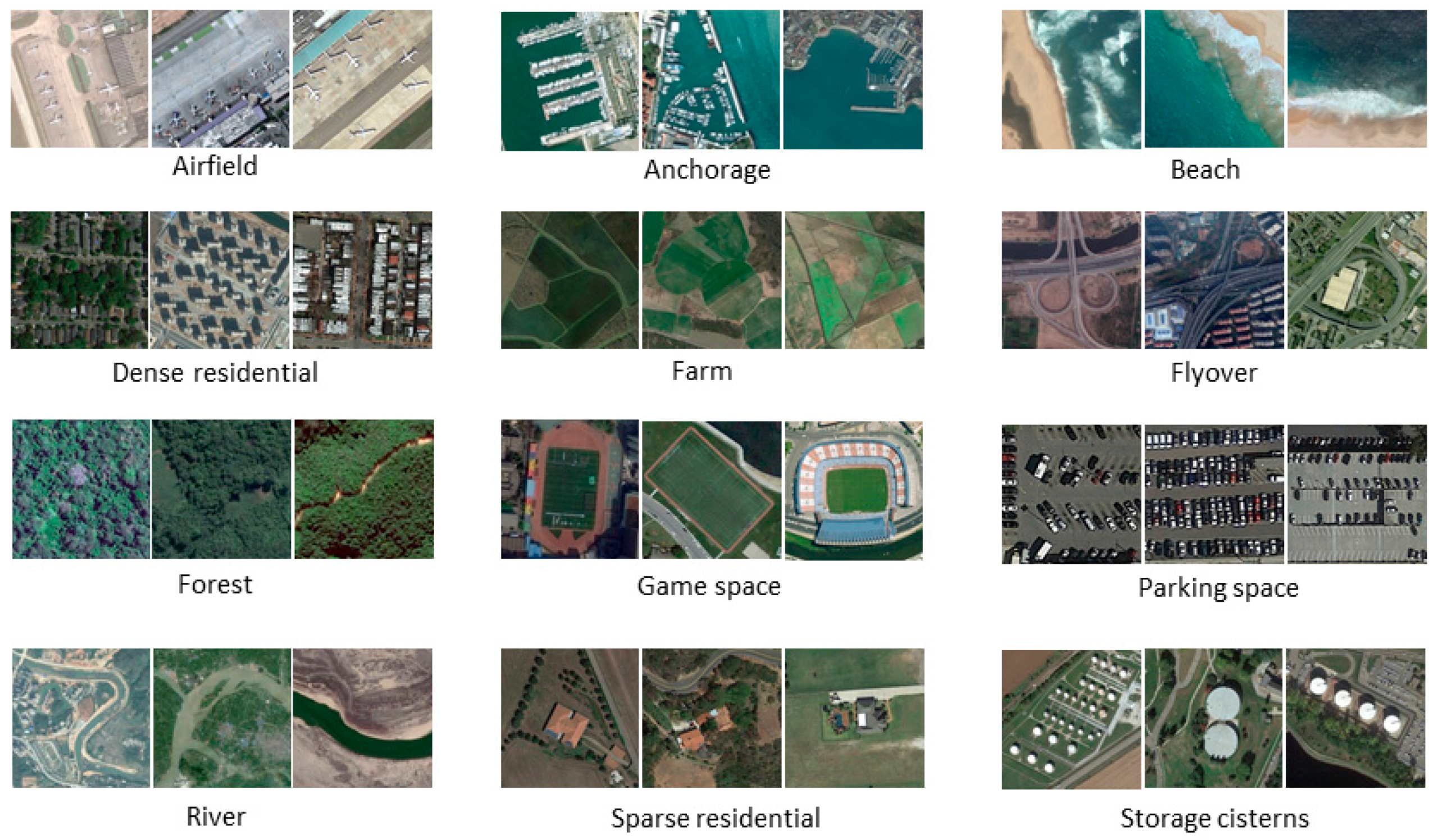
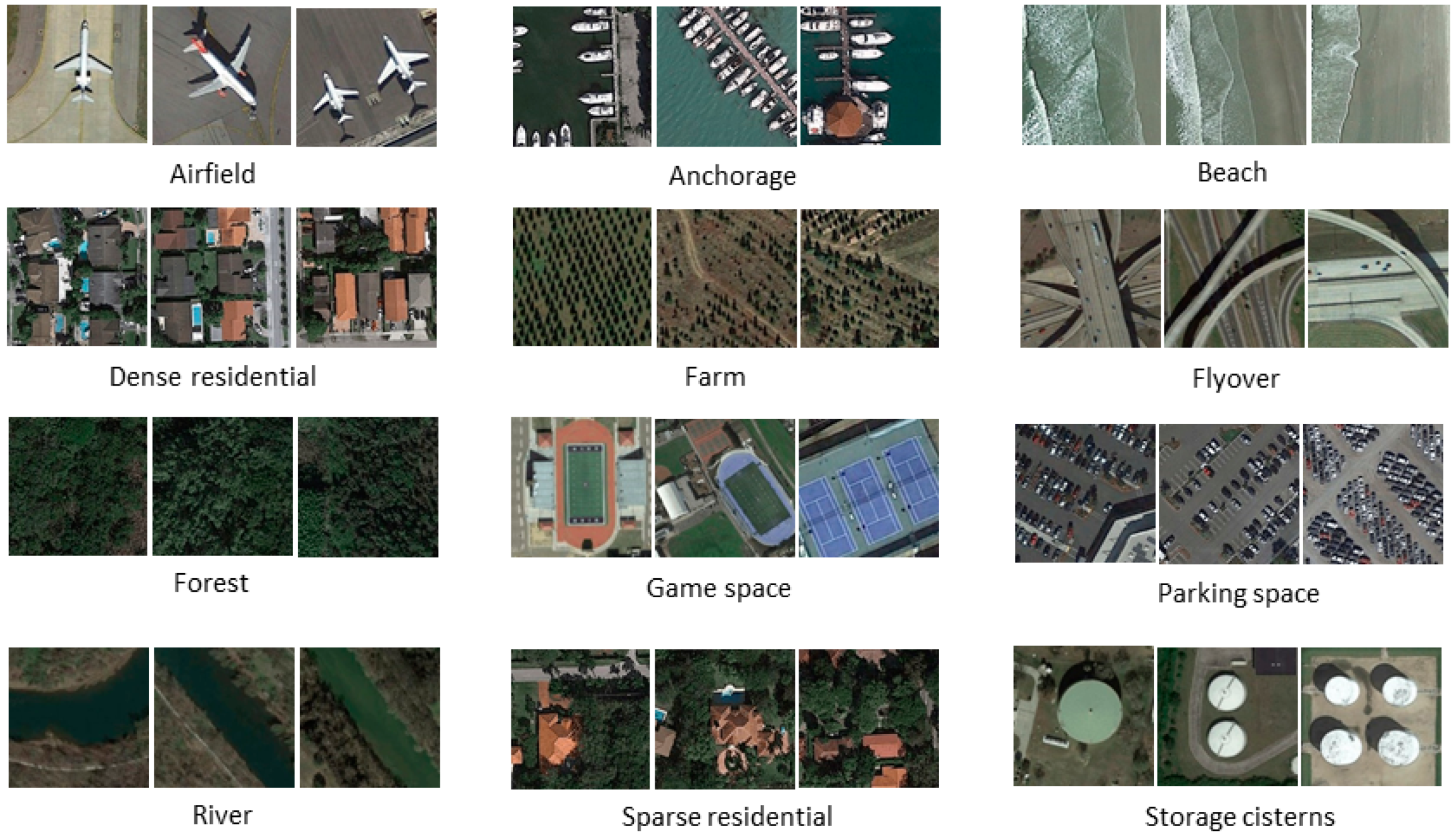
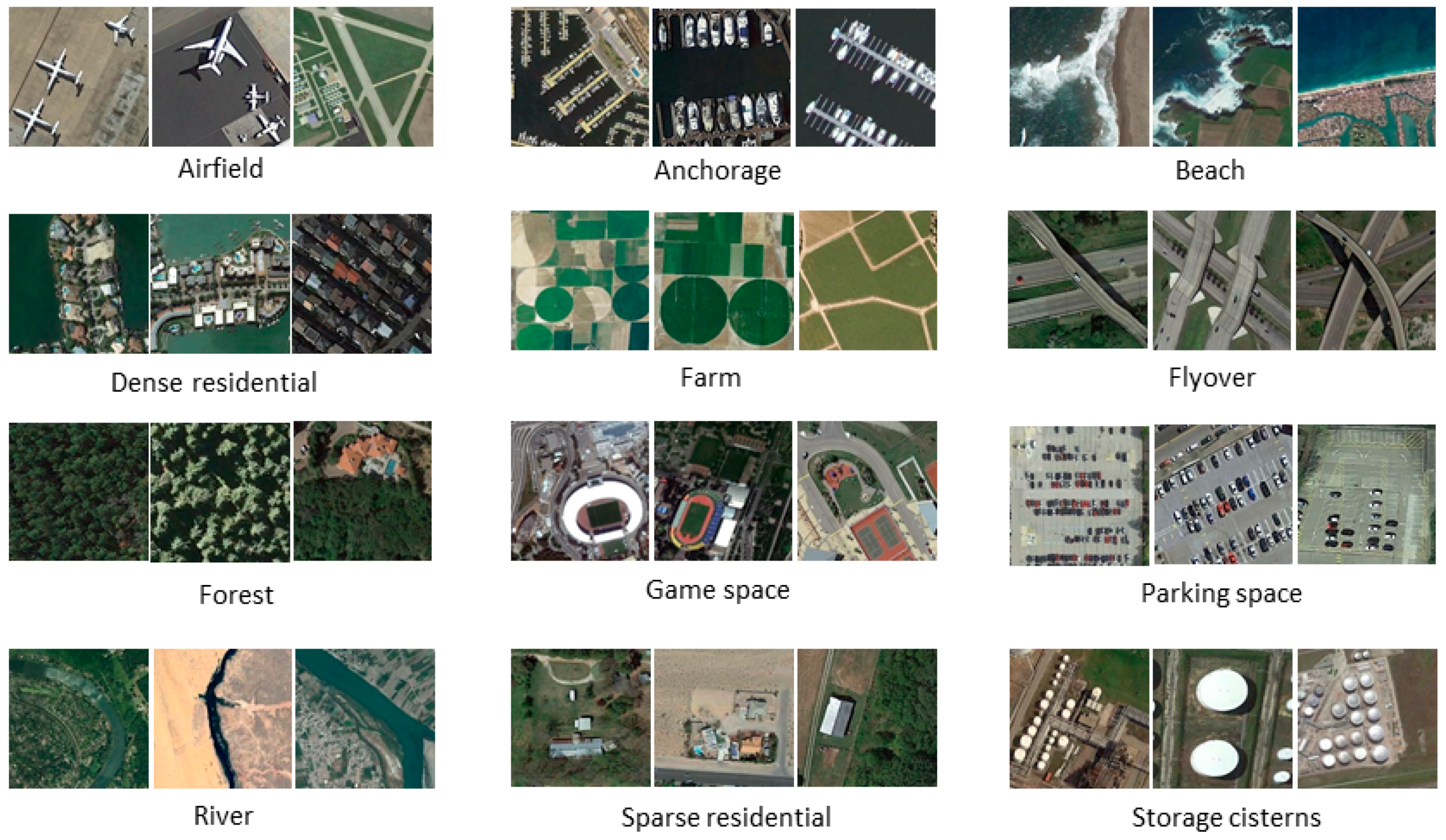
3.1. Description of the Multisource Dataset
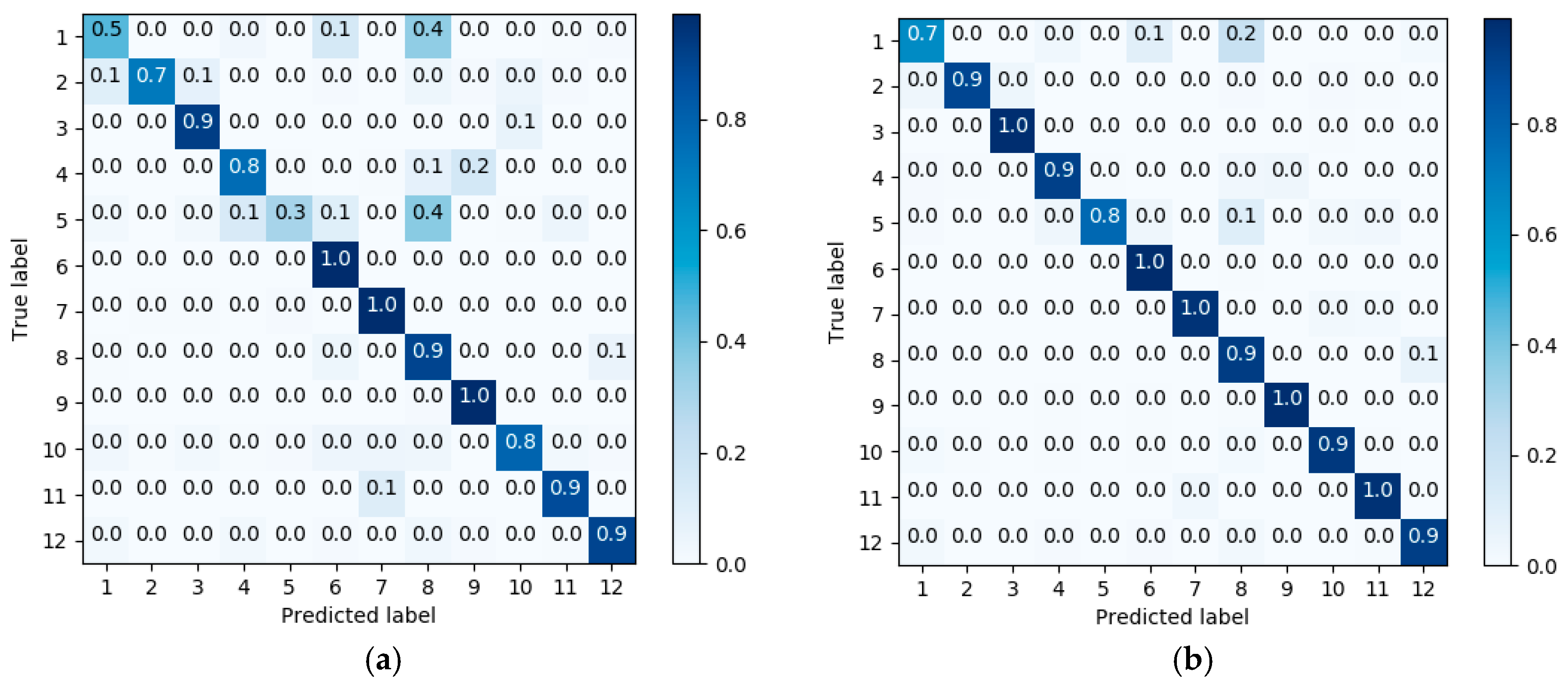
3.2. Results
4. Discussion
5. Conclusions
Author Contributions
Funding
Acknowledgments
Conflicts of Interest
References
- Foody, G.M. Remote sensing of tropical forest environments: Towards the monitoring of environmental resources for sustainable development. Int. J. Remote Sens. 2003, 24, 4035–4046. [Google Scholar] [CrossRef]
- Moranduzzo, T.; Mekhalfi, M.L.; Melgani, F. LBP-based multiclass classification method for UAV imagery. In Proceedings of the 2015 IEEE International Geoscience and Remote Sensing Symposium (IGARSS), Milan, Italy, 26–31 July 2015; pp. 2362–2365. [Google Scholar]
- Dean, A.M.; Smith, G.M. An evaluation of per-parcel land cover mapping using maximum likelihood class probabilities. Int. J. Remote Sens. 2003, 24, 2905–2920. [Google Scholar] [CrossRef]
- Myint, S.W.; Gober, P.; Brazel, A.; Grossman-Clarke, S.; Weng, Q. Per-pixel vs. object-based classification of urban land cover extraction using high spatial resolution imagery. Remote Sens. Environ. 2011, 115, 1145–1161. [Google Scholar] [CrossRef]
- Chen, Y.; Zhou, Y.; Ge, Y.; An, R.; Chen, Y. Enhancing Land Cover Mapping through Integration of Pixel-Based and Object-Based Classifications from Remotely Sensed Imagery. Remote Sens. 2018, 10, 77. [Google Scholar] [CrossRef]
- Zhai, D.; Dong, J.; Cadisch, G.; Wang, M.; Kou, W.; Xu, J.; Xiao, X.; Abbas, S. Comparison of Pixel- and Object-Based Approaches in Phenology-Based Rubber Plantation Mapping in Fragmented Landscapes. Remote Sens. 2017, 10, 44. [Google Scholar] [CrossRef]
- Lopes, M.; Fauvel, M.; Girard, S.; Sheeren, D. Object-based classification of grasslands from high resolution satellite image time series using Gaussian mean map kernels. Remote Sens. 2017, 9. [Google Scholar] [CrossRef]
- Zerrouki, N.; Bouchaffra, D. Pixel-based or Object-based: Which approach is more appropriate for remote sensing image classification? In Proceedings of the 2014 IEEE International Conference on Systems, Man, and Cybernetics (SMC), Qufu, China, 10–12 August 2014; pp. 864–869. [Google Scholar]
- Gonçalves, F.M.F.; Guilherme, I.R.; Pedronette, D.C.G. Semantic Guided Interactive Image Retrieval for plant identification. Expert Syst. Appl. 2018, 91, 12–26. [Google Scholar] [CrossRef]
- Demir, B.; Bruzzone, L. A Novel Active Learning Method in Relevance Feedback for Content-Based Remote Sensing Image Retrieval. IEEE Trans. Geosci. Remote Sens. 2015, 53, 2323–2334. [Google Scholar] [CrossRef]
- Zhao, L.J.; Tang, P.; Huo, L.Z. Land-Use Scene Classification Using a Concentric Circle-Structured Multiscale Bag-of-Visual-Words Model. IEEE J. Sel. Top. Appl. Earth Obs. Remote Sens. 2014, 7, 4620–4631. [Google Scholar] [CrossRef]
- Mekhalfi, M.L.; Melgani, F.; Bazi, Y.; Alajlan, N. Land-Use Classification with Compressive Sensing Multifeature Fusion. IEEE Geosci. Remote Sens. Lett. 2015, 12, 2155–2159. [Google Scholar] [CrossRef]
- Qi, K.; Wu, H.; Shen, C.; Gong, J. Land-Use Scene Classification in High-Resolution Remote Sensing Images Using Improved Correlatons. IEEE Geosci. Remote Sens. Lett. 2015, 12, 2403–2407. [Google Scholar] [CrossRef]
- Chen, C.; Zhang, B.; Su, H.; Li, W.; Wang, L. Land-use scene classification using multi-scale completed local binary patterns. Signal Image Video Process. 2016, 10, 745–752. [Google Scholar] [CrossRef]
- Chen, S.; Tian, Y. Pyramid of Spatial Relatons for Scene-Level Land Use Classification. IEEE Trans. Geosci. Remote Sens. 2015, 53, 1947–1957. [Google Scholar] [CrossRef]
- Chen, C.; Zhou, L.; Guo, J.; Li, W.; Su, H.; Guo, F. Gabor-Filtering-Based Completed Local Binary Patterns for Land-Use Scene Classification. In Proceedings of the 2015 IEEE International Conference on Multimedia Big Data, Beijing, China, 20–22 April 2015; pp. 324–329. [Google Scholar]
- Zhang, F.; Du, B.; Zhang, L. Scene Classification via a Gradient Boosting Random Convolutional Network Framework. IEEE Trans. Geosci. Remote Sens. 2016, 54, 1793–1802. [Google Scholar] [CrossRef]
- Zhang, L.; Zhang, L.; Du, B. Deep Learning for Remote Sensing Data: A Technical Tutorial on the State of the Art. IEEE Geosci. Remote Sens. Mag. 2016, 4, 22–40. [Google Scholar] [CrossRef]
- Zhang, F.; Du, B.; Zhang, L. Saliency-Guided Unsupervised Feature Learning for Scene Classification. IEEE Trans. Geosci. Remote Sens. 2015, 53, 2175–2184. [Google Scholar] [CrossRef]
- Zou, Q.; Ni, L.; Zhang, T.; Wang, Q. Deep Learning Based Feature Selection for Remote Sensing Scene Classification. IEEE Geosci. Remote Sens. Lett. 2015, 12, 2321–2325. [Google Scholar] [CrossRef]
- Nogueira, K.; Penatti, O.A.B.; dos Santos, J.A. Towards Better Exploiting Convolutional Neural Networks for Remote Sensing Scene Classification. Pattern Recognit. 2017, 61, 539–556. [Google Scholar] [CrossRef]
- Sherrah, J. Fully Convolutional Networks for Dense Semantic Labelling of High-Resolution Aerial Imagery. arXiv, 2016; arXiv:1606.02585. [Google Scholar]
- Lyu, H.; Lu, H. A deep information based transfer learning method to detect annual urban dynamics of Beijing and Newyork from 1984–2016. In Proceedings of the 2017 IEEE International Geoscience and Remote Sensing Symposium (IGARSS), Fort Worth, TX, USA, 23–28 July 2017; pp. 1958–1961. [Google Scholar]
- Kendall, A.; Badrinarayanan, V.; Cipolla, R. Bayesian SegNet: Model Uncertainty in Deep Convolutional Encoder-Decoder Architectures for Scene Understanding. arXiv, 2015; arXiv:1511.02680. [Google Scholar]
- Mou, L.; Schmitt, M.; Wang, Y.; Zhu, X.X. A CNN for the identification of corresponding patches in SAR and optical imagery of urban scenes. In Proceedings of the 2017 Joint Urban Remote Sensing Event (JURSE), Dubai, UAE, 6–8 March 2017; pp. 1–4. [Google Scholar]
- Cheng, G.; Li, Z.; Yao, X.; Guo, L.; Wei, Z. Remote Sensing Image Scene Classification Using Bag of Convolutional Features. IEEE Geosci. Remote Sens. Lett. 2017, 14, 1735–1739. [Google Scholar] [CrossRef]
- Kussul, N.; Lavreniuk, M.; Skakun, S.; Shelestov, A. Deep Learning Classification of Land Cover and Crop Types Using Remote Sensing Data. IEEE Geosci. Remote Sens. Lett. 2017, 14, 778–782. [Google Scholar] [CrossRef]
- Weng, Q.; Mao, Z.; Lin, J.; Liao, X. Land-use scene classification based on a CNN using a constrained extreme learning machine. Int. J. Remote Sens. 2018. [Google Scholar] [CrossRef]
- Yu, X.; Wu, X.; Luo, C.; Ren, P. Deep learning in remote sensing scene classification: A data augmentation enhanced convolutional neural network framework. GISci. Remote Sens. 2017, 54, 741–758. [Google Scholar] [CrossRef]
- Sun, S.; Shi, H.; Wu, Y. A survey of multi-source domain adaptation. Inf. Fusion 2015, 24, 84–92. [Google Scholar] [CrossRef]
- Ganin, Y.; Ustinova, E.; Ajakan, H.; Germain, P.; Larochelle, H.; Laviolette, F.; Marchand, M.; Lempitsky, V. Domain-Adversarial Training of Neural Networks. In Domain Adaptation in Computer Vision Applications; Advances in Computer Vision and Pattern Recognition; Springer: Cham, Switzerland, 2017; pp. 189–209. ISBN 978-3-319-58346-4. [Google Scholar]
- Xu, S.; Mu, X.; Chai, D.; Wang, S. Adapting Remote Sensing to New Domain with ELM Parameter Transfer. IEEE Geosci. Remote Sens. Lett. 2017, 14, 1618–1622. [Google Scholar] [CrossRef]
- Ye, M.; Qian, Y.; Zhou, J.; Tang, Y.Y. Dictionary Learning-Based Feature-Level Domain Adaptation for Cross-Scene Hyperspectral Image Classification. IEEE Trans. Geosci. Remote Sens. 2017, 55, 1544–1562. [Google Scholar] [CrossRef]
- Patel, V.M.; Gopalan, R.; Li, R.; Chellappa, R. Visual Domain Adaptation: A survey of recent advances. IEEE Signal Process. Mag. 2015, 32, 53–69. [Google Scholar] [CrossRef]
- Blitzer, J.; Dredze, M.; Pereira, F. Biographies, Bollywood, Boom-boxes and Blenders: Domain Adaptation for Sentiment Classification. In Proceedings of the ACL 2007—45th Annual Meeting of the Association for Computational Linguistics, Prague, Czech Republic, 23–30 June 2007. [Google Scholar]
- Shimodaira, H. Improving predictive inference under covariate shift by weighting the log-likelihood function. J. Stat. Plan. Inference 2000, 90, 227–244. [Google Scholar] [CrossRef]
- Sugiyama, M.; Nakajima, S.; Kashima, H.; von Bünau, P.; Kawanabe, M. Direct Importance Estimation with Model Selection and Its Application to Covariate Shift Adaptation. In Proceedings of the Neural Information Processing Systems, Vancouver, BC, Canada, 3–6 December 2007; Volume 20. [Google Scholar]
- Duan, L.; Tsang, I.W.; Xu, D.; Maybank, S.J. Domain Transfer SVM for video concept detection. In Proceedings of the 2009 IEEE Conference on Computer Vision and Pattern Recognition, Miami, FL, USA, 20–25 June 2009; pp. 1375–1381. [Google Scholar]
- Pan, S.J.; Kwok, J.T.; Yang, Q. Transfer Learning via Dimensionality Reduction. In Proceedings of the 23rd National Conference on Artificial Intelligence, AAAI’08, Chicago, IL, USA, 13–17 July 2008; AAAI Press: Chicago, IL, USA, 2008; Volume 2, pp. 677–682. [Google Scholar]
- Long, M.; Wang, J.; Cao, Y.; Sun, J.; Yu, P.S. Deep Learning of Transferable Representation for Scalable Domain Adaptation. IEEE Trans. Knowl. Data Eng. 2016, 28, 2027–2040. [Google Scholar] [CrossRef]
- Ganin, Y.; Lempitsky, V. Unsupervised Domain Adaptation by Backpropagation. In Proceedings of the International Conference on Machine Learning, Lille, France, 6–11 July 2015; pp. 1180–1189. [Google Scholar]
- Long, M.; Cao, Y.; Wang, J.; Jordan, M.I. Learning Transferable Features with Deep Adaptation Networks. In Proceedings of the 32nd International Conference on International Conference on Machine Learning, ICML’15, Lille, France, 6–11 July 2015; JMLR.org: Lille, France, 2015; Volume 37, pp. 97–105. [Google Scholar]
- Kuzborskij, I.; Maria Carlucci, F.; Caputo, B. When Naive Bayes Nearest Neighbors Meet Convolutional Neural Networks. In Proceedings of the IEEE Conference on Computer Vision and Pattern Recognition, Las Vegas, NV, USA, 27–30 June 2016; pp. 2100–2109. [Google Scholar]
- Wang, Y.-X.; Hebert, M. Learning to Learn: Model Regression Networks for Easy Small Sample Learning. In Proceedings of the Computer Vision—ECCV 2016, Amsterdam, The Netherlands, 11–14 October 2016; Lecture Notes in Computer Science. Springer: Cham, Switzerland, 2016; pp. 616–634. [Google Scholar]
- Chen, Q.; Huang, J.; Feris, R.; Brown, L.M.; Dong, J.; Yan, S. Deep domain adaptation for describing people based on fine-grained clothing attributes. In Proceedings of the 2015 IEEE Conference on Computer Vision and Pattern Recognition (CVPR), Boston, MA, USA, 7–12 June 2015; pp. 5315–5324. [Google Scholar]
- Long, M.; Zhu, H.; Wang, J.; Jordan, M.I. Unsupervised Domain Adaptation with Residual Transfer Networks. arXiv, 2016; arXiv:1602.04433. [Google Scholar]
- Sun, B.; Saenko, K. Deep CORAL: Correlation Alignment for Deep Domain Adaptation. In Proceedings of the Computer Vision, ECCV 2016 Workshops, Amsterdam, The Netherlands, 11–14 October 2016; Lecture Notes in Computer Science. Springer: Cham, Switzerland, 2016; pp. 443–450. [Google Scholar]
- Wang, Y.; Li, W.; Dai, D.; Van Gool, L. Deep Domain Adaptation by Geodesic Distance Minimization. arXiv, 2017; arXiv:1707.09842. [Google Scholar]
- Tzeng, E.; Hoffman, J.; Saenko, K.; Darrell, T. Adversarial Discriminative Domain Adaptation (workshop extended abstract). arXiv, 2017; arXiv:1702.05464. [Google Scholar]
- Luo, P.; Zhuang, F.; Xiong, H.; Xiong, Y.; He, Q. Transfer Learning from Multiple Source Domains via Consensus Regularization. In Proceedings of the 17th ACM Conference on Information and Knowledge Management, CIKM’08, Napa Valley, CA, USA, 26–30 October 2008; ACM: New York, NY, USA, 2008; pp. 103–112. [Google Scholar]
- Schweikert, G.; Widmer, C.; Schölkopf, B.; Rätsch, G. An Empirical Analysis of Domain Adaptation Algorithms for Genomic Sequence Analysis. In Proceedings of the 21st International Conference on Neural Information Processing Systems, NIPS’08, Vancouver, BC, Canada, 3–6 December 2007; pp. 1433–1440. [Google Scholar]
- Duan, L.; Tsang, I.W.; Xu, D.; Chua, T.-S. Domain Adaptation from Multiple Sources via Auxiliary Classifiers. In Proceedings of the 26th Annual International Conference on Machine Learning, ICML’09, Montreal, QC, Canada, 14–18 June 2009; ACM: New York, NY, USA, 2009; pp. 289–296. [Google Scholar]
- Chattopadhyay, R.; Sun, Q.; Fan, W.; Davidson, I.; Panchanathan, S.; Ye, J. Multisource Domain Adaptation and Its Application to Early Detection of Fatigue. ACM Trans. Knowl. Discov. Data 2012, 6, 1–26. [Google Scholar] [CrossRef]
- Crammer, K.; Kearns, M.; Wortman, J. Learning from Multiple Sources. J. Mach. Learn. Res. 2008, 9, 1757–1774. [Google Scholar]
- Hoffman, J.; Kulis, B.; Darrell, T.; Saenko, K. Discovering Latent Domains for Multisource Domain Adaptation. In Proceedings of the Computer Vision—ECCV 2012, Florence, Italy, 7–13 October 2012; Lecture Notes in Computer Science. Springer: Berlin/Heidelberg, Germany, 2012; pp. 702–715, ISBN 978-3-642-33708-6. [Google Scholar]
- Kulis, B.; Saenko, K.; Darrell, T. What you saw is not what you get: Domain adaptation using asymmetric kernel transforms. In Proceedings of the CVPR 2011, Springs, CO, USA, 20–25 June 2011; pp. 1785–1792. [Google Scholar]
- Duan, L.; Xu, D.; Tsang, I.W.H.; Luo, J. Visual Event Recognition in Videos by Learning from Web Data. IEEE Trans. Pattern Anal. Mach. Intell. 2012, 34, 1667–1680. [Google Scholar] [CrossRef] [PubMed]
- Othman, E.; Bazi, Y.; Melgani, F.; Alhichri, H.; Alajlan, N.; Zuair, M. Domain Adaptation Network for Cross-Scene Classification. IEEE Trans. Geosci. Remote Sens. 2017, 55, 4441–4456. [Google Scholar] [CrossRef]
- Bashmal, L.; Bazi, Y.; AlHichri, H.; AlRahhal, M.; Ammour, N.; Alajlan, N.; Bashmal, L.; Bazi, Y.; AlHichri, H.; AlRahhal, M.M.; et al. Siamese-GAN: Learning Invariant Representations for Aerial Vehicle Image Categorization. Remote Sens. 2018, 10, 351. [Google Scholar] [CrossRef]
- Ammour, N.; Bashmal, L.; Bazi, Y.; Rahhal, M.M.A.; Zuair, M. Asymmetric Adaptation of Deep Features for Cross-Domain Classification in Remote Sensing Imagery. IEEE Geosci. Remote Sens. Lett. 2018, 15, 597–601. [Google Scholar] [CrossRef]
- Yang, Y.; Newsam, S. Bag-of-visual-words and Spatial Extensions for Land-use Classification. In Proceedings of the 18th SIGSPATIAL International Conference on Advances in Geographic Information Systems, GIS’10, San Jose, CA, USA, 3–5 November 2010; ACM: New York, NY, USA, 2010; pp. 270–279. [Google Scholar]
- Xia, G.; Hu, J.; Hu, F.; Shi, B.; Bai, X.; Zhong, Y.; Zhang, L.; Lu, X. AID: A Benchmark Data Set for Performance Evaluation of Aerial Scene Classification. IEEE Trans. Geosci. Remote Sens. 2017, 55, 3965–3981. [Google Scholar] [CrossRef]
- Zhou, W.; Newsam, S.; Li, C.; Shao, Z. PatternNet: A benchmark dataset for performance evaluation of remote sensing image retrieval. ISPRS J. Photogramm. Remote Sens. 2018. [Google Scholar] [CrossRef]
- Cheng, G.; Han, J.; Lu, X. Remote Sensing Image Scene Classification: Benchmark and State of the Art. Proc. IEEE 2017, 105, 1865–1883. [Google Scholar] [CrossRef]
- He, K.; Zhang, X.; Ren, S.; Sun, J. Deep Residual Learning for Image Recognition. In Proceedings of the 2016 IEEE Conference on Computer Vision and Pattern Recognition (CVPR), Las Vegas, NV, USA, 26 June–1 July 2016; pp. 770–778. [Google Scholar]
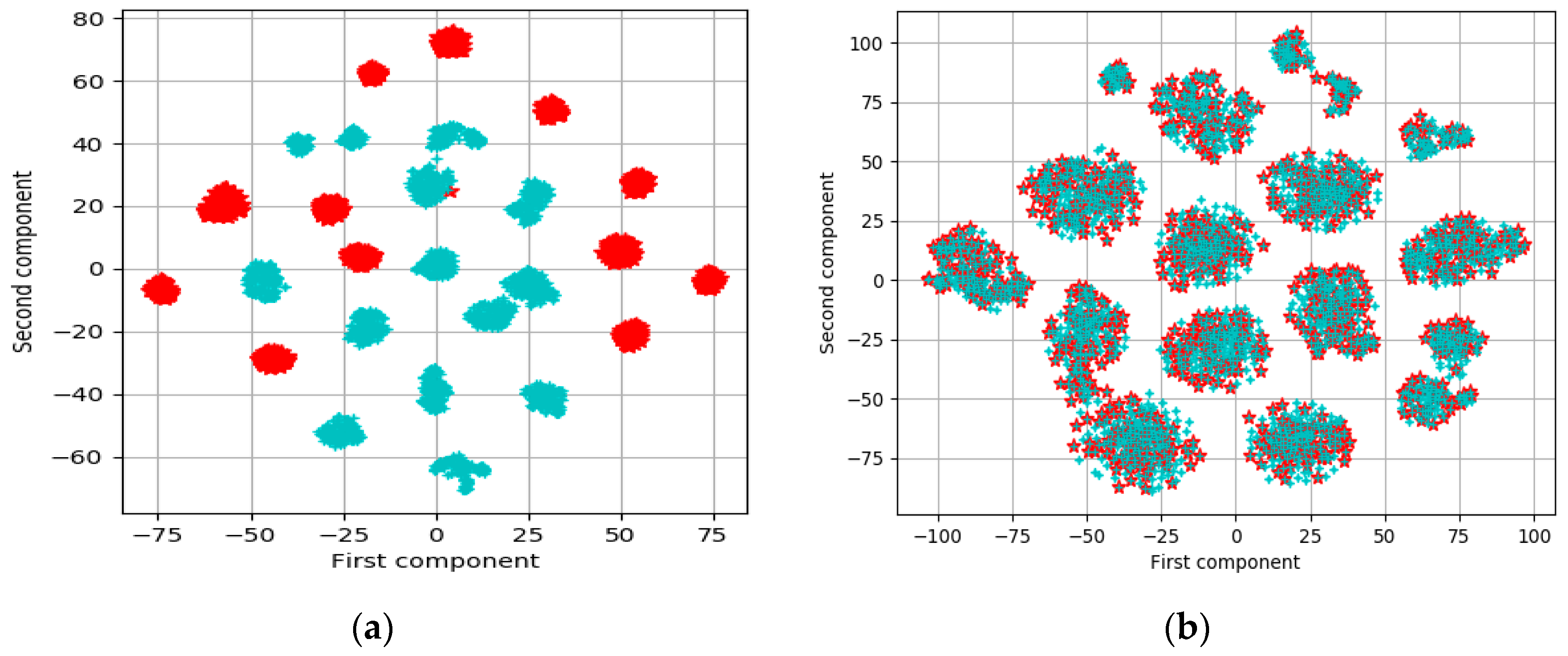
- van der Maaten, L.; Hinton, G. Visualizing Data using t-SNE. J. Mach. Learn. Res. 2008, 9, 2579–2605. [Google Scholar]


| Class | Merced | AID | PatternNet | NWPU |
|---|---|---|---|---|
| Airfield | 100 | 360 | 800 | 1400 |
| Anchorage | 100 | 380 | 800 | 700 |
| Beach | 100 | 400 | 800 | 700 |
| Dense Residential | 100 | 410 | 800 | 700 |
| Farm | 100 | 370 | 800 | 1400 |
| Flyover | 100 | 420 | 800 | 700 |
| Forest | 100 | 250 | 800 | 700 |
| Game Space | 100 | 660 | 1600 | 1400 |
| Parking Space | 100 | 390 | 800 | 700 |
| River | 100 | 410 | 800 | 700 |
| Sparse Residential | 100 | 300 | 800 | 700 |
| Storage Cisterns | 100 | 360 | 800 | 700 |
| Total | 1200 | 4710 | 10,400 | 10,500 |
| (a) | ||||
| Source Datasets | ||||
| Merced | NWPU | PatternNet | Fusion Layer | |
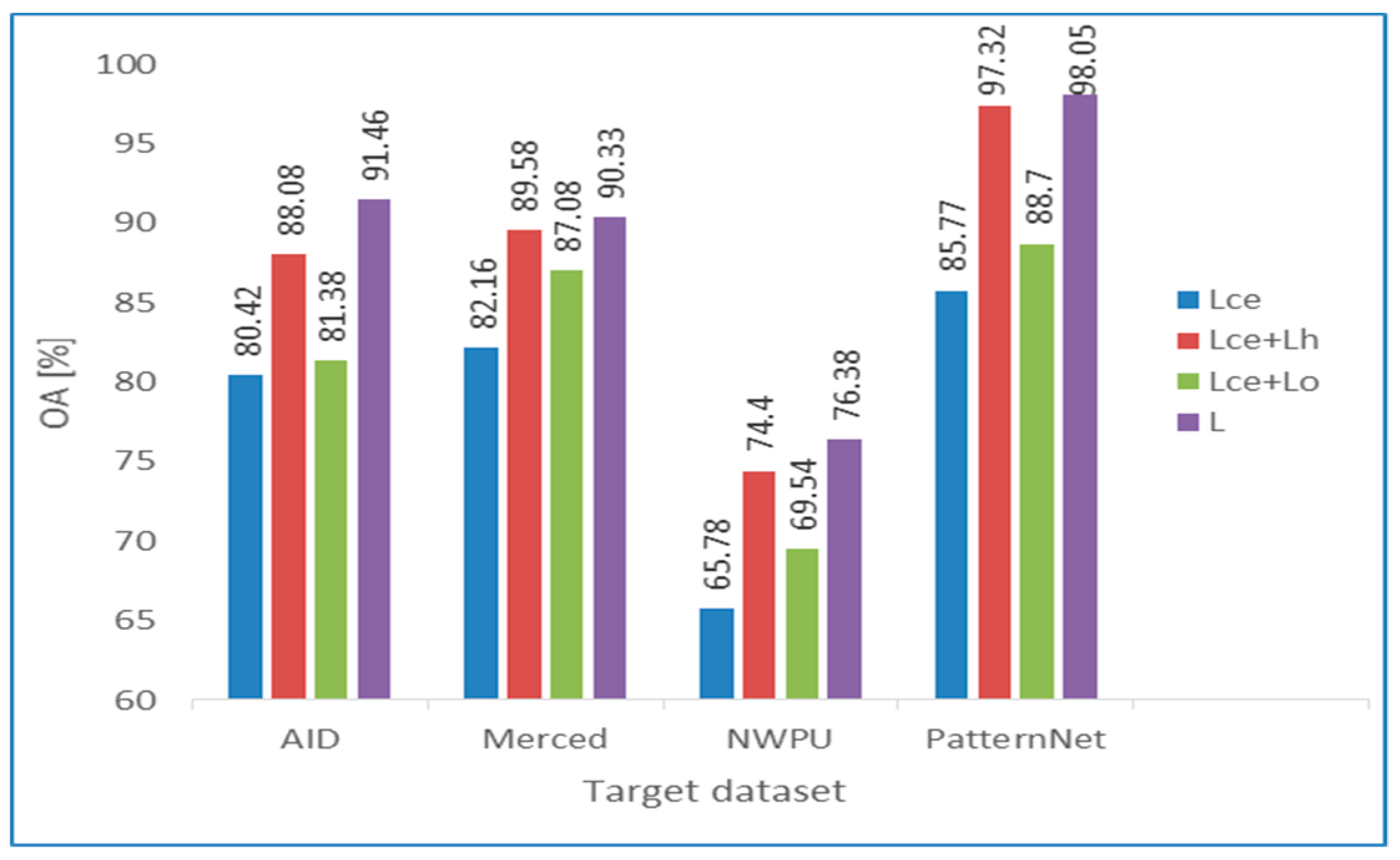
| Lce | 58.13 | 91.46 | 61.50 | 80.42 |
| L = Lce + Lh + Lo | 81.63 | 95.32 | 80.95 | 91.46 |
| (b) | ||||
| Source Datasets | ||||
| AID | NWPU | PatternNet | Fusion Layer | |
| Lce | 69.33 | 68.50 | 83.66 | 82.16 |
| L = Lce + Lh + Lo | 83.99 | 85.83 | 91.83 | 90.33 |
| (c) | ||||
| Source Datasets | ||||
| AID | Merced | PatternNet | Fusion Layer | |
| Lce | 75.86 | 54.54 | 55.57 | 65.78 |
| L = Lce + Lh + Lo | 87.69 | 68.25 | 61.39 | 76.38 |
| (d) | ||||
| Source Datasets | ||||
| AID | Merced | NWPU | Fusion Layer | |
| Lce | 68.14 | 93.58 | 75.54 | 85.77 |
| L = Lce + Lh + Lo | 90.84 | 99.41 | 84.25 | 98.05 |
© 2018 by the authors. Licensee MDPI, Basel, Switzerland. This article is an open access article distributed under the terms and conditions of the Creative Commons Attribution (CC BY) license (http://creativecommons.org/licenses/by/4.0/).
Share and Cite
Al Rahhal, M.M.; Bazi, Y.; Abdullah, T.; Mekhalfi, M.L.; AlHichri, H.; Zuair, M. Learning a Multi-Branch Neural Network from Multiple Sources for Knowledge Adaptation in Remote Sensing Imagery. Remote Sens. 2018, 10, 1890. https://doi.org/10.3390/rs10121890
Al Rahhal MM, Bazi Y, Abdullah T, Mekhalfi ML, AlHichri H, Zuair M. Learning a Multi-Branch Neural Network from Multiple Sources for Knowledge Adaptation in Remote Sensing Imagery. Remote Sensing. 2018; 10(12):1890. https://doi.org/10.3390/rs10121890
Chicago/Turabian StyleAl Rahhal, Mohamad M., Yakoub Bazi, Taghreed Abdullah, Mohamed L. Mekhalfi, Haikel AlHichri, and Mansour Zuair. 2018. "Learning a Multi-Branch Neural Network from Multiple Sources for Knowledge Adaptation in Remote Sensing Imagery" Remote Sensing 10, no. 12: 1890. https://doi.org/10.3390/rs10121890
APA StyleAl Rahhal, M. M., Bazi, Y., Abdullah, T., Mekhalfi, M. L., AlHichri, H., & Zuair, M. (2018). Learning a Multi-Branch Neural Network from Multiple Sources for Knowledge Adaptation in Remote Sensing Imagery. Remote Sensing, 10(12), 1890. https://doi.org/10.3390/rs10121890